Big Black Hole, Little Neutron Star:Magnetic Dipole Fields in the Rindler Spacetime

Abstract

As a black hole and neutron star approach during inspiral, the field lines of a magnetized neutron star eventually thread the black hole event horizon and a short-lived electromagnetic circuit is established. The black hole acts as a battery that provides power to the circuit, thereby lighting up the pair just before merger. Although originally suggested as an electromagnetic counterpart to gravitational-wave detection, a black hole battery is of more general interest as a novel luminous astrophysical source. To aid in the theoretical understanding, we present analytic solutions for the electromagnetic fields of a magnetic dipole in the presence of an event horizon. In the limit that the neutron star is very close to a Schwarzschild horizon, the Rindler limit, we can solve Maxwell’s equations exactly for a magnetic dipole on an arbitrary worldline. We present these solutions here and investigate a proxy for a small segment of the neutron star orbit around a big black hole. We find that the voltage the black hole battery can provide is in the range $\sim 10^{16}$ statvolts with a projected luminosity of $10^{42}$ ergs/s for an $M=10M_{\odot}$ black hole, a neutron star with a B-field of $10^{12}G$, and an orbital velocity $\sim 0.5c$ at a distance of $3M$ from the horizon. Larger black holes provide less power for binary separations at a fixed number of gravitational radii. The black hole/neutron star system therefore has a significant power supply to light up various elements in the circuit possibly powering bursts, jets, beamed radiation, or even a hot spot on the neutron star crust.

I Introduction

Although intrinsically dark, a black hole (BH) can potentially act as a battery in an electromagnetic circuit – a battery that can power great luminosities when connected to other elements in the circuit (MacDonald and Thorne, 1982).

Blandford-Znajek famously proposed a BH battery as the power source for quasar jets Blandford and Znajek (1977). In their well-known model, a spinning BH twists a strong magnetic field anchored in an accretion disk to create an emf that powers an energetic jet. The BH spins down as energy is lost to the luminosity of the jet. In a related yet novel scenario, it was recently proposed McWilliams and Levin (2011) that a magnetized neutron star (NS) in orbit with a BH could light up. When the BH orbits within the magnetosphere of the NS, the relative motion of the BH through the NS dipole field could generate an emf. The BH acts as a battery, the field lines as wires, the charged particles of the NS magnetosphere as current carriers, and the NS itself behaves as a resistor. In principle, the orbit would wind down as angular momentum is lost to the circuit, although in practice gravitational radiation drains angular momentum by far the faster. The circuit is illustrated schematically in Figure 1. (See also Refs. Piro (2012); Lai (2012); Lyutikov (2011); Palenzuela et al. (2010, 2013) for related systems.)

Figure 1: Neutron star - Rindler horizon effective circuit diagram. Magnetic field lines act as wires connecting the neutron star to the horizon. Current flows in (out) of the horizon via positively (negatively) charged particles spiraling in tight Larmor radii around magnetic field lines into the horizon.

BH-NS pairs may generate gamma-ray bursts during merger via the Blandford-Znajek mechansim; when the NS is tidally disrupted, accreting material tows a magnetic field into the ringing BH (Narayan et al., 1992; Lee et al., 2005; Faber et al., 2006; Shibata and Uryu, 2007; Shibata and Taniguchi, 2008; Etienne et al., 2009; Rezzolla et al., 2011; Etienne et al., 2012; East et al., 2012; Giacomazzo et al., 2013). If the BH is big enough, however, the NS will not be tidally disrupted prior to merger but instead will be swallowed whole, prohibiting the post-merger gamma-ray burst. Since AdLIGO will be most sensitive to binaries with larger BH’s (Harry and LIGO Scientific Collaboration, 2010), it is important to note that the electromagnetic circuit of (McWilliams and Levin, 2011) may be the only electromagnetic counterpart to the gravitational-wave signal.

In this paper, we describe the BH-NS circuit in an analytic calculation valid for large BHs. Very near a large BH, the event horizon looks like a flat wall and in this limit the Schwarzschild metric can be approximated by a Rindler metric – the metric of a flat spacetime as measured by observers with uniform proper-accelerations. In the Rindler limit, calculations are simplified while some of the key physics is retained. Due to acceleration, the Rindler observer also sees a flat-wall event horizon and so the relevant interaction of the EM field with an horizon is present. Also, since the Rindler observer is just on a special worldline in flat spacetime, calculations can be carried out in the Minkowski spacetime and transformed to Rindler, a significant calculational advantage. (The Rindler limit is also used by (MacDonald and Suen, 1985) to investigate the fields of a point charge interacting with an horizon.)

We consider a magnetic dipole on an arbitrary worldline near the flat-wall event horizon and derive analytic expressions for the electromagnetic fields. We find that a battery is established when the worldline of the source incorporates motion parallel to the horizon and the pair have approached within the light cylinder of the NS. As the pair draws closer under the effects of gravitational radiation, the power of the battery and luminosity of the circuit hits a maximum, just prior to merger. We evaluate the maximum power the black-hole battery would provide to a completed circuit, and thus the maximum luminosity generated. In addition, we estimate the maximum energy to which plasma particles could be accelerated, and thus the type of emission the circuit is capable of producing. As a preview of the conclusions, we quote here the rough scaling of the voltage and luminosity:

$$V^{\rm{max}}_{\mathcal{H}} \sim 3.3\times 10^{16}\left(\frac{B_{p}}{10^{12}\ \rm{G}}\right)\left(\frac{M}{10M_{\odot}}\right)^{-2}\rm{statvolts}$$

$$\mathcal{L}^{\rm{max}} \sim 1.3\times 10^{42}\left(\frac{B_{p}}{10^{12}\ \rm{G}}\right)^{2}\left(\frac{M}{10M_{\odot}}\right)^{-4}\frac{\rm{erg}}{\rm{s}}$$ (1)

where $M$ is the mass of the BH and $B_{p}$ is the magnetic field strength at the poles of the NS. (Readers who prefer to skip the derivations in favor of the conclusions can fast-forward to the results of §VIII.) These scalings only apply at a fixed height $3M$ above the horizon and are dependent on the unknown resistivities of the plasma and of the NS. Eqs. (1) should therefore be taken as a guide only. Still, even with these caveats, the conclusion is that a BH-NS circuit could power high-energy bursts of radiation visible to current missions, especially for the special case of magnetar-strength NS fields. This intriguing possibility calls for more detailed predictions of the timescales and spectra of emission, a topic for future explorations. We hope that, in addition to the above estimates, the electro-vacuum example this paper provides will be a resource for further analytic studies and numerical experiments.

II Set-up and Limits

II.1 Rindler Spacetime

Consider the line element in Minkowski spacetime

$$ds^{2}=-dT^{2}+dX^{2}+dY^{2}+dZ^{2}\ \$$ (2)

The following coordinate transformation,

$$T =z\hbox{sinh}(g_{H}t)\hbox{ }\hbox{ }\hbox{ }\hbox{ }\hbox{ }\hbox{ }\hbox{ }X=x$$

$$Z =z\hbox{cosh}(g_{H}t)\hbox{ }\hbox{ }\hbox{ }\hbox{ }\hbox{ }\hbox{ }Y=y,$$ (3)

leads to the Rindler line element,

$$ds^{2} =-\alpha^{2}dt^{2}+dx^{2}+dy^{2}+dz^{2}$$

$$\alpha =g_{H}z$$ (4)

where the lapse function $\alpha$ measures the difference in Rindler observer proper time $\tau_{R}$ and Rindler coordinate time $t$. For reference, the inverse transformation is given by

$$t =\frac{1}{g_{H}}\tanh^{-1}\left[\frac{T}{Z}\right]$$

$$z =\sqrt{Z^{2}-T^{2}},$$ (5)

and we may write the non-inertial, uniformly accelerated trajectory in Minkowski coordinates as,

$$X^{\mu}_{R} =(T,0,0,Z)=(z_{R}\sinh(g_{H}t),0,0,z_{R}\cosh(g_{H}t))$$

$$u_{R}^{\mu} =\frac{dX_{R}}{d\tau_{R}}=(\gamma_{R},0,0,\gamma_{R}\beta_{R})$$

$$a_{R}^{\mu} =\frac{du_{R}}{d\tau_{R}}=z_{R}^{-1}(\gamma_{R}\beta_{R},0,0,\gamma_{R})$$ (6)

where

$$\beta_{R} =\frac{dZ}{dT}=\frac{T}{Z}$$

$$\gamma_{R} =(1-\beta_{R}^{2})^{-1/2}\ .$$ (7)

It is also useful to express these in Rindler coordinates

$$\gamma_{R} =\cosh(g_{H}t)$$

$$\gamma_{R}\beta_{R} =\sinh(g_{H}t)\ .$$ (8)

The 4-acceleration has constant magnitude:

$$a_{R}^{\mu}a^{R}_{\mu}=z_{R}^{-2}$$ (9)

and so observers of constant Rindler coordinate $z_{R}$ have a $4$-acceleration of constant magnitude according to a Minkowski observer.

Figure 2: Rindler space is the shaded wedge given by $T>\pm Z$, $Z>0$ on the Minkowski spacetime diagram. The dotted vertical line is the trajectory of a Minkowski observer and the dashed hyperbolic line is that of a Rindler observer as viewed by a Minkowski observer. In the frame of the Rindler observer an event horizon exists at $T=\pm Z$.

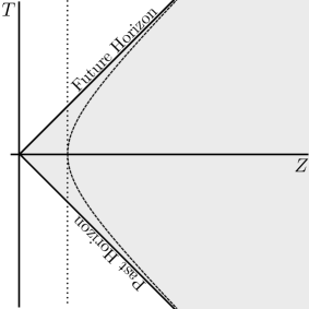
Figure 2 is a Minkowski spacetime diagram demonstrating the wedge occupied by the Rindler spacetime (shaded region). The worldline of a stationary Minkowski observer is denoted by the vertical dotted line while the worldline of a Rindler observer is denoted by the dashed hyperbolic trajectory (Eqs. (6)). Due to their accelerations, Rindler observers are causally disconnected from the non-shaded region of Minkowski space in Figure 2 and thus experience an event horizon at $z=0$ ($T=\pm Z$, $Z>0$).

With the choice of $g_{H}=1/(4M)$ and the transformations,

$$x=2M\phi\quad y=2M\left(\theta-\pi/2\right)\quad z=4M\left(1-2M/r\right)^{1/2}$$ (10)

the Rindler line element approximates the Schwarzschild line element around the point $(r,\phi,\theta)=(2M,0,\pi/2)$. Errors of order unity in the approximation to the Schwarzschild spacetime occur when $z\rightarrow 4M$ ($\alpha\rightarrow 1$) and $y\rightarrow 2M$ (see e.g. (MacDonald and Suen, 1985)). The Rindler limit retains some key features of the spacetime, including gravitational red-shifting and time dilation as well as the event horizon, although it necessarily misses elements of spatial curvature.

II.2 Electrodynamical Properties of an Event Horizon and the Horizon Battery

To understand and interpret power generation by the BH-NS circuit, we first review some key features of horizon electrodynamics Thorne et al. (1986). We consult observers who are at a fixed location relative to the event horizon. These fiducial observers can tell us if the event horizon has established charge separation and therefore a battery. Around a BH, these observers must accelerate to maintain a fixed location and avoid plunging into the BH. Similarly, in Rindler space, our fiducial observers accelerate to maintain a fixed location $z$ from the event horizon. So while stationary relative to the horizon, our fiducial observers are not stationary in an absolute sense – they are non-inertial and so must burn fuel to stay at their Rindler-coordinate location.

We are therefore after the electric ${\bf E}_{R}$ and magnetic ${\bf B}_{R}$ fields measured by a Rindler observer – fields due to a magnetic dipole source on an arbitrary worldline – and we want to determine these fields everywhere outside the event horizon. Problematically, the fields of a Rindler observer will necessarily experience divergences at the event horizon due to infinite time dilation. Following the membrane paradigm Thorne et al. (1986), we construct a timelike hyper-surface stretched over the true, null-horizon. On the stretched horizon, fields will be finite. We then apply electromagnetic boundary conditions on this fictitious surface. Since electric field lines can only terminate or originate on sources, the stretched horizon is assigned hypothetical surface charge to satisfy the boundary conditions of any normal ${\bf E}_{R}$ component. Similarly, the stretched horizon is assigned hypothetical surface current to satisfy the boundary conditions of any tangential ${\bf B}_{R}$ component. As can be derived from local versions of Gauss’s law and Ampere’s law, the fictitious charge density and surface current are given by

$$\mathbf{E_{R}}\cdot\mathbf{n}\big{|}_{\mathcal{H}}=4\pi\sigma_{\mathcal{H}}\qquad\alpha\mathbf{B_{R}}\big{|}_{\mathcal{H}}=4\pi\mathbf{\mathcal{J}_{\mathcal{H}}}\times\mathbf{n}$$ (11)

where $\mathbf{n}$ is the unit normal to the horizon and $\mathcal{H}$ denotes evaluation at the stretched horizon. The interpretation then is that electric fields terminate on charges in the stretched horizon, and magnetic fields parallel to the horizon are sourced by surface currents.

Combining (11) along with the horizon normal component of the differential form of Ampere’s law gives charge conservation on the horizon

$$\frac{\partial\sigma_{\mathcal{H}}}{\partial t}+\nabla\cdot\mathbf{\mathcal{J}_{\mathcal{H}}}=-\left(\alpha j_{n}\right)_{\mathcal{H}}$$ (12)

where $\left(\alpha j_{n}\right)_{\mathcal{H}}$ is the normal component of currents entering (positive charges flowing in) and leaving (negative charges flowing in) the horizon in units of universal time. The divergence is the two-dimensional divergence computed on the horizon.

The lesson of the membrane paradigm: when electromagnetic field boundary conditions are applied, the horizon behaves as if it were a conductor with the resistivity of free space. On this (hypothetical) conductor may exist (hypothetical) surface charges and currents. Eq. (12) tells us that charge is conserved as current flows. In the vacuum calculations presented here, the right hand side of (12) will always be zero (to fractional errors of order $\alpha_{\mathcal{H}}$ arising from stretching the horizon) as there is no plasma to carry current off the horizon.

We will be particularly interested in the case where the motion of a magnetic field relative to the Rindler observers induces an electric field that has normal components to the horizon. These normal components source a surface charge density on the horizon that must, when integrated over the black hole area, amount to zero net charge for an initially uncharged black hole. Therefore, charge separation is induced on the horizon and that gradient can be interpreted as creating a battery. If an external circuit is connected to the horizon then the horizon emf associated with the charge separation will drive a current in the circuit. The instantaneous emf of such a horizon battery is given by

$$V_{\mathcal{H}}=\int{\left[\alpha\mathbf{E_{R}}\right]_{\mathcal{H}}\cdot ds}\ ,$$ (13)

remembering that an electric potential is only well-defined for electric fields that originate and terminate on source charges, albeit hypothetical source charges in this case. The situation is analogous to a conventional chemical battery. In the horizon battery, energy of motion of the magnetic field source replaces the chemical energy. In the specific case of a NS orbiting a Schwarzschild BH, the energy source is the spin and orbital energy of the binary.

Figure 1 shows the equivalent electrical circuit of such a system. The horizon battery drives current in the form of charged magnetosphere particles spiraling along the NS magnetic field lines. Current enters the horizon via positive-charge carriers (positrons) riding magnetic field lines into the horizon and leaves the horizon via negative-charge carriers (electrons) flowing into the horizon. The current flows through three resistors comprised of the NS, the plasma, and the BH. If we know the electric field induced from the orbital motion of the magnetic dipole we can compute an horizon battery voltage. We may calculate the power, as observed at infinity, dissipated by the $i^{th}$ resistive component of the system,

$$\mathcal{P}=\frac{V^{2}_{\mathcal{H}}}{(\mathcal{R}_{\mathcal{H}}+\mathcal{R}_{NS}+2\mathcal{R}_{\rm{plasma}})^{2}}\mathcal{R}_{i},$$ (14)

to approximate the luminosity generated by that component. While the resistance of the BH horizon is set by the resistivity of free space Thorne et al. (1986), the resistances of the NS and plasma are interesting unknowns. Although the primary calculations done here are all in vacuum, in §VIII we use Eq. (14) to estimate the power and find that there is potential for significant bursts of energy from black hole batteries.

First, we find exact closed form solutions for the electromagnetic fields of a magnetic dipole on an arbitrary worldline. We then implement those solutions for specific dipole trajectories.

III A magnetic Dipole in arbitrary motion

III.1 The Electromagnetic Four-Potential

In Minkowski spacetime, Maxwell’s equations for the 4-potential $A^{\alpha}$ are,

$$\Box A^{\alpha}({x})-\partial^{\alpha}\left(\partial_{\beta}A^{\beta}\right)=\frac{4\pi}{c}J^{\alpha}({x})$$ (15)

where $J^{\alpha}({x})$ is the 4-current as a function of the coordinates. We choose to work in the Lorentz Gauge $\partial_{\beta}A^{\beta}=0$. Then Maxwell’s equations for the 4-potential become sourced wave-equations,

$$\Box A^{\alpha}({x})=\frac{4\pi}{c}J^{\alpha}({x}).$$ (16)

We choose the 4-current for a point dipole source

$$J^{\alpha}({x})=\hbox{ }\nabla_{\mu}\int{Q^{\alpha\mu}(\tau)\delta^{(4)}\left[{x}-{x_{S}}(\tau)\right]d\tau}$$ (17)

where $\tau$ is the proper time of the dipole source, not to be confused with the proper time of the Rindler observers $\tau_{R}$, and the antisymmetric dipole tensor,

$$Q^{\alpha\mu}(\tau) =V^{\alpha}p^{\mu}-p^{\alpha}V^{\mu}+\epsilon^{\alpha\mu}_{\hbox{ }\hbox{ }\hbox{ }\rho\sigma}V^{\rho}m^{\sigma},$$ (18)

is the decomposition of electric $p$ and magnetic $m$ parts (Ribaric and Sustersic, 1995; Peter Rowe and Rowe, 1987). (See appendix §B for more detail.) Notice that $V$ is the instantaneous 4-velocity of the source. Also, hereafter $X$ will denote observer coordinates and $X_{S}$ will denote the coordinates along the trajectory of the dipole source. The antisymmetric tensor is fixed by $\epsilon^{0123}=1$.

The solution for $A^{\alpha}$ is derived in Appendix A and can be written in the Minkowski frame, off of the worldline of the source, as

$$A^{\alpha} =\nabla_{\mu}\left[\frac{Q^{\alpha\mu}}{r\cdot V}\right]_{*}\ \ .$$ (19)

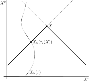
By $r\cdot V$ between 4-vectors we mean the inner product $g_{\mu\nu}r^{\mu}V^{\nu}$. Since the source may be moving, we must account for the fact that an observer at $X$ will observe fields due to the source in the past, it taking the speed of light for the source information to get to the observer. Therefore, the 4-potential is always evaluated at the retarded time $T_{*}$ as represented graphically in Figure 3.

Figure 3: Diagram demonstrating the relationship between source trajectory coordinates $X_{S}(\tau)$, observer coordinates $X$, and the retarded proper time $\tau_{*}(X)$ at the intersection of the past light cone of an observer at $X$ and the source trajectory.

The retarded time is found as a function of observer coordinates by imposing the null condition. We define the relative distance between an observer and a point on the source trajectory in Minkowski coordinates as

$$r^{\mu}=\begin{pmatrix}r^{0}\\ {\bf{r}}\end{pmatrix}\equiv\begin{pmatrix}T-T_{S}\\ {\bf{X}}-{\bf{X}}_{S}(T_{S})\end{pmatrix}\quad.$$ (20)

The null condition is $(r_{\mu}r^{\mu})_{*}=0$, with subscript $*$ denoting evaluation at $T_{*}$. Then

$$r^{0}=\sqrt{{\bf r}\cdot{\bf r}}=r$$ (21)

and

$$({\bf{X}}-{\bf{X}}_{S}(T_{*}))^{2}=(T-T_{*})^{2}\quad.$$ (22)

It should be noted that the covariant derivative in (19) is taken with respect to the coordinates $X^{\mu}$. Since the solution to the null condition for $T_{*}$ is dependent on the position of the observer, $T_{*}=T_{*}(X^{\mu})$, $T_{*}$ is acted on by the covariant derivative.

For completeness, we expand the 4-potential further. Since $(r_{\mu}r^{\mu})_{*}=0$ we may write,

$$r_{\mu}\nabla_{\nu}r^{\mu}|_{*}=0=r_{\mu}\left(\delta^{\mu}_{\nu}-\nabla_{\nu}\tau\ V^{\mu}\right)|_{*}=r_{\nu}-(r\cdot V)\nabla_{\nu}\tau|_{*}\quad.$$

Given this extremely useful relation, we can compile a list of gradients that we will need in order to evaluate Eq. (19) and construct the field tensor:

$$\nabla_{\mu}\tau =\frac{r_{\mu}}{(r\cdot V)}$$

$$\nabla_{\mu}r^{\nu} =\delta_{\mu}^{\nu}-\frac{r_{\mu}\ V^{\nu}}{(r\cdot V)}$$

$$\nabla_{\mu}V^{\nu} =\frac{r_{\mu}\ a^{\nu}}{(r\cdot V)}$$

$$\nabla_{\mu}a^{\nu} =\frac{r_{\mu}}{(r\cdot V)}\dot{a}^{\nu}$$

$$\nabla_{\mu}m^{\nu} =\frac{r_{\mu}}{(r\cdot V)}\dot{m}^{\nu}$$ (23)

where an overdot denotes a $\tau$ derivative. Evaluation at $*$ is implied in the relations (23).

When there is only a magnetic dipole moment ${\bf m}$, then $Q^{\alpha\mu}=\epsilon^{\alpha\mu}_{\quad\ \ \rho\sigma}V^{\rho}m^{\sigma}$ and we can expand the 4-potential as:

$$A^{\alpha}(x) =\epsilon^{\alpha}_{\quad\mu\rho\sigma}r^{\mu}\left[\frac{a^{\rho}m^{\sigma}+V^{\rho}\dot{m}^{\sigma}}{(r\cdot V)^{2}}-\frac{V^{\rho}m^{\sigma}(1+r\cdot a)}{(r\cdot V)^{3}}\right]\Bigg{|}_{*}\ .$$ (24)

Note that the RHS of Eq. (24) reduces to the usual stationary dipole solution for a constant dipole at rest ($V^{\alpha}=(1,0,0,0)$ and $\dot{m}=0$), as it must.

Given the 4-potential, the electromagnetic field tensor is

$$F_{\alpha\beta}=\nabla_{[\alpha}A_{\beta]}=\nabla_{\alpha}A_{\beta}-\nabla_{\beta}A_{\alpha}$$ (25)

Using (23) and (24) to evaluate (25) we find

$$F_{\alpha\beta}(x) =-\epsilon_{[\alpha\beta]\rho\sigma}\frac{a^{\rho}m^{\sigma}+V^{\rho}\dot{m}^{\sigma}}{(r\cdot V)^{2}}$$

$$+\frac{r_{[\alpha}\epsilon_{\beta]\mu\rho\sigma}}{(r\cdot V)^{3}}\Big{\{}r^{\mu}\left(2a^{\rho}\dot{m}^{\sigma}+V^{\rho}\ddot{m}^{\sigma}+\dot{a}^{\rho}m^{\sigma}\right)-V^{\mu}\left(a^{\rho}m^{\sigma}+V^{\rho}\dot{m}^{\sigma}\right)\Big{\}}$$

$$-2\frac{V_{[\alpha}\epsilon_{\beta]\mu\rho\sigma}}{(r\cdot V)^{3}}\Big{\{}r^{\mu}\left(a^{\rho}m^{\sigma}+V^{\rho}\dot{m}^{\sigma}\right)\Big{\}}-\frac{a_{[\alpha}\epsilon_{\beta]\mu\rho\sigma}}{(r\cdot V)^{3}}r^{\mu}V^{\rho}m^{\sigma}+\epsilon_{[\alpha\beta]\rho\sigma}\frac{V^{\rho}m^{\sigma}}{(r\cdot V)^{3}}(1+r\cdot a)$$

$$-\frac{r_{[\alpha}\epsilon_{\beta]\mu\rho\sigma}}{(r\cdot V)^{4}}\Big{\{}3r^{\mu}\left(a^{\rho}m^{\sigma}+V^{\rho}\dot{m}^{\sigma}\right)(1+r\cdot a)+r^{\mu}V^{\rho}m^{\sigma}(r\cdot\dot{a})-V^{\mu}V^{\rho}m^{\sigma}(1+r\cdot a)\Big{\}}$$

$$+3\frac{V_{[\alpha}\epsilon_{\beta]\mu\rho\sigma}}{(r\cdot V)^{4}}r^{\mu}V^{\rho}m^{\sigma}(1+r\cdot a)$$

$$+3\frac{r_{[\alpha}\epsilon_{\beta]\mu\rho\sigma}}{(r\cdot V)^{5}}r^{\mu}V^{\rho}m^{\sigma}(1+r\cdot a)^{2}.$$ (26)

Again, evaluation at $*$ is implied in the expression (26).

The electromagnetic fields for an observer with 4-velocity $u^{\beta}$ are

$$E^{\alpha}=F^{\alpha\mu}u_{\mu}\qquad B^{\alpha}=\frac{1}{2}\epsilon^{\alpha\mu\gamma\delta}F_{\gamma\delta}u_{\mu}$$ (27)

A stationary Minkowski observer has 4-velocity $u^{\mu}=(1,0,0,0)$ and the Minkowski fields drop out:

$${\bf E}_{M} =-{\mathbf{\nabla}}A^{0}-\nabla_{0}{\bf A}$$

$${\bf B}_{M} ={\mathbf{\nabla}}\times{\bf A}\quad.$$ (28)

In vector notation,

$$A^{0}= \frac{\left(\mathbf{a}\times\mathbf{m}\right)\cdot\mathbf{r}+\left(\mathbf{V}\times\mathbf{\dot{m}}\right)\cdot\mathbf{r}}{(r\cdot V)^{2}}-\frac{\left(\mathbf{V}\times\mathbf{m}\right)\cdot\mathbf{r}}{(r\cdot V)^{3}}\left(1+r\cdot a\right)\quad\bigg{|}_{*}$$

$$\mathbf{A}= \frac{r^{0}\left(\mathbf{a}\times\mathbf{m}\right)+r^{0}\left(\mathbf{V}\times\mathbf{\dot{m}}\right)-a^{0}\left(\mathbf{r}\times\mathbf{m}\right)-V^{0}\left(\mathbf{r}\times\mathbf{\dot{m}}\right)+m^{0}\left(\mathbf{r}\times\mathbf{a}\right)+\dot{m}^{0}\left(\mathbf{r}\times\mathbf{V}\right)}{(r\cdot V)^{2}}\Bigg{|}_{*}$$

$$- \frac{r^{0}(\mathbf{V}\times\mathbf{m})-V^{0}(\mathbf{m}\times\mathbf{r})+m^{0}\left(\mathbf{r}\times\mathbf{V}\right)}{(r\cdot V)^{3}}\left(1+r\cdot a\right)\Bigg{|}_{*}$$ (29)

where the source kinematics can be expressed as

$$V^{\alpha} =(V^{0},\bf{V})=(\gamma_{S},\gamma_{S}\boldsymbol{\beta}_{S})$$ (30)

$${\boldsymbol{\beta}}_{S} =\frac{d\mathbf{X}_{S}}{dT}$$

$$a^{\alpha} =\left(\gamma_{S}^{4}\left({\boldsymbol{\beta}}_{S}\cdot\frac{d{\boldsymbol{\beta}}_{S}}{dT}\right),\gamma_{S}^{2}\frac{d{\boldsymbol{\beta}}_{S}}{dT}+\gamma_{S}^{4}\left({\boldsymbol{\beta}}_{S}\cdot\frac{d{\boldsymbol{\beta}}_{S}}{dT}\right){\boldsymbol{\beta}}_{S}\right)$$

where $\gamma_{S}$, ${\boldsymbol{\beta}}_{S}$ are the instantaneous Lorentz factor and Lorentz boost of the source, not to be confused with $\gamma_{R}$, $\beta_{R}$ of the Rindler observer. A dipole with only a magnetic rest frame moment $\bf{m_{S}}$ moving at ${\boldsymbol{\beta}}$ relative to our Minkowski observer has moments

$$p^{\alpha} =\left(0,\vec{0}\right)$$ (31)

$$m^{\alpha} =\left(\gamma_{S}{\boldsymbol{\beta}}_{S}\cdot{\bf{m_{S}}},{\bf{m_{S}}}+(\gamma_{S}-1)(\hat{\boldsymbol{\beta}}_{S}\cdot\mathbf{m_{S}})\hat{\boldsymbol{\beta}}_{S}\right)$$

as explained in more detail in appendix B. With the values in Eqs. (30)-(31), the Minkowski fields can be computed. Rindler fields are then transformed from the Minkowski fields.

We find the Rindler fields ${\bf E}_{R}$ and ${\bf B}_{R}$ (primed) expressed in terms of Minkowski fields ${\bf E}_{M},{\bf B}_{M}$ (unprimed) and the Rindler 4-velocity (6) via the transformations,

$$E^{\alpha^{\prime}}=\frac{\partial x^{\alpha^{\prime}}}{\partial x^{\alpha}}F^{\alpha\mu}u^{R}_{\mu}\hbox{ }\hbox{ }\hbox{ }\hbox{ }\hbox{ }\hbox{ }B^{\alpha^{\prime}}=\frac{1}{2}\frac{\partial x^{\alpha^{\prime}}}{\partial x^{\alpha}}\epsilon^{\alpha\mu\gamma\delta}F_{\gamma\delta}u^{R}_{\mu}.$$ (32)

Here $u_{R}^{\mu}$ is the Rindler velocity according to a Minkowski observer and the coordinate transformation expresses the components of the fields in the Rindler basis.

A compact way to expand Eqs. (32) exploits the fact that any vector can be decomposed as

$${\bf E}_{R} =\hat{\boldsymbol{\beta}}_{R}(\hat{\boldsymbol{\beta}}_{R}\cdot{\bf E}_{R})+\hat{\boldsymbol{\beta}}_{R}\times({\bf E}_{R}\times\hat{\boldsymbol{\beta}}_{R})$$

$$={\bf E}_{R}^{\perp}+{\bf E}_{R}^{\parallel}$$ (33)

where $\perp$ and $\parallel$ refer to components perpendicular to the Rindler horizon and parallel to the Rindler horizon respectively. (So $\perp$ is parallel to ${\boldsymbol{\beta}}_{R}$ and $\parallel$ is perpendicular to ${\boldsymbol{\beta}}_{R}$.) The fields as measured by a Rindler observer are then expressed conveniently in terms of the fields as measured by a Minkowski observer as

$${\bf E}_{R} ={\bf E}_{M}^{\perp}+\gamma_{R}{\bf E}_{M}^{\parallel}+\gamma_{R}({\boldsymbol{\beta}}_{R}\times{\bf B}_{M}^{\parallel})$$

$${\bf B}_{R} ={\bf B}_{M}^{\perp}+\gamma_{R}{\bf B}_{M}^{\parallel}-\gamma_{R}({\boldsymbol{\beta}}_{R}\times{\bf E}_{M}^{\parallel})\quad.$$ (34)

Although we will focus on computing a charge gradient on the horizon to gauge the power output of the BH-circuit in the following examples, it is also instructive to consider the Poynting flux driven by the Rindler dipole. Given the electromagnetic fields as measured by the Rindler observer, we may compute the Poynting vector in Rindler space as seen by an observer at infinity,

$$\mathbf{S}=\frac{\alpha^{2}}{4\pi}\mathbf{E}_{R}\times\mathbf{B}_{R},$$ (35)

where one factor of $\alpha$ converts from locally measured energy to energy at infinity and the second factor converts from proper time measured by the local stationary observer to the universal time of the 3+1 split (see §II.2).

To understand the meaning of the Poynting flux in this case, we integrate Poynting’s theorem over the entire Rindler 3-volume, bounded at infinity and the horizon,

$$\frac{dU}{dt}=-\int{\mathbf{S}_{\infty}\cdot dA}-\int{\mathbf{E}_{H}\cdot\mathbf{\mathcal{J}_{H}}\hbox{ }dA}.$$ (36)

The last term on the right is evaluated over the stretched horizon since this is the only location in the volume where there are non-zero currents (we could of course add a plasma and get more currents). In the absence of radiation at infinity, we see that any change in EM energy $U$ must be due to ohmic dissipation from horizon surface currents.

Generally, the Poynting flux perceived by a Rindler observer can be expressed in terms of Minkowski fields as

$$4\pi\alpha^{-2}{\bf S}= \gamma_{R}E_{M}^{\perp}\left[(\hat{\boldsymbol{\beta}}_{R}\times{\bf B}_{M}^{\parallel})+\beta_{R}{\bf E}_{M}^{\parallel}\right]$$

$$+\gamma_{R}B_{M}^{\perp}\left[-(\hat{\boldsymbol{\beta}}_{R}\times{\bf E}_{M}^{\parallel})+\beta_{R}{\bf B}_{M}^{\parallel}\right]$$

$$-\gamma_{R}^{2}{\boldsymbol{\beta}}_{R}\left[(B_{M}^{\parallel})^{2}+(E_{M}^{\parallel})^{2}\right]$$

$$+\gamma_{R}^{2}\left(1+{\boldsymbol{\beta}}_{R}^{2}\right)\left[{\bf E}_{M}^{\parallel}\times{\bf B}_{M}^{\parallel}\right]$$ (37)

The first two terms represent flux parallel to the horizon. The third term is always into the horizon and is due solely to the Rindler motion. The final term can be in or out of the horizon and is proportional to the in or out ($\pm Z$) Poynting flux that would be observed by a Minkowski observer. This final term is the only term that could contribute to power coming out of the dipole-horizon system. However, it can be negated by the inward flux do to Rindler observer motion.

In our vacuum calculations, the Poynting flux can only tell us about radiation from the moving dipole fields, since we have not included a plasma. Instead, we look for the existence of a battery to ascertain if there is a power source. When a magnetosphere is added, the black-hole battery will power an outward Poynting flux at infinity delivering radiation to a distant observer.

IV A Freely Falling Dipole Solution

As a check of the above dipole solutions, we consider a dipole source that is stationary in Minkowski space at the location $(X_{S}=0,Y_{S}=0,Z_{S}=$constant). According to the Rindler observer, the magnetic dipole appears to fall straight into the event horizon. In Minkowski coordinates, the world line is characterized by

$$r^{\alpha} =\begin{pmatrix}T-T_{S}\\ X\\ Y\\ Z-Z_{S}\end{pmatrix}$$

$$V^{\alpha} =\begin{pmatrix}1\\ 0\\ 0\\ 0\end{pmatrix}\qquad a^{\alpha}=\begin{pmatrix}0\\ 0\\ 0\\ 0\end{pmatrix}.$$ (38)

The trajectory is plotted as the dotted worldline in Figure 4 as seen by Minkowski observers (top panel) and by Rindler observers (bottom panel). The retarded time can be found in closed form:

$$T_{*}=T-\sqrt{X^{2}+Y^{2}+(Z-Z_{S})^{2}}\ .$$

Because our source is stationary in Minkowski spacetime, there is no dependence on $T$ in the field solutions and

$$\left(r\cdot V\right)_{*}=-r_{*}$$ (39)

$\begin{array}[]{c}\includegraphics[scale={0.33}]{Inf_Stat_STDiagram.pdf}\\ \includegraphics[scale={0.33}]{InfandStat_Rind_stDiagram.pdf}\end{array}$

Figure 4: Spacetime diagrams for the infalling Rindler dipole of section §IV. Also shown is the worldline of a Rindler observer. The top panel is drawn by Minkowski observers, the bottom panel is drawn by Rindler observers. Note that $Z_{S}=z_{S}$ at $T=t=0$, hence the labeling of the initial source position.

Then our 4-potential becomes simply

$$A^{\alpha}(x)=\frac{\epsilon^{\alpha}_{\quad\mu 0\sigma}r^{\mu}m^{\sigma}}{r^{3}}\bigg{|}_{*}$$ (40)

which, written more familiarly, is the potential of a stationary magnetic dipole

$$A^{0}=0,\quad{\bf{A}}(x)=\frac{\bf{m_{S}}\times\hat{\bf{r}}}{r^{2}}.$$ (41)

where $\hat{\bf{r}}=\textbf{r}/r$ and ${\bf{m_{S}}}$ is the source 3-dipole moment.

The nonzero field components as viewed by the Minkowski observer in the rest frame of the dipole are

$${\bf E}_{M} =0$$

$${\bf B}_{M} =\frac{\left[3(\bf{m_{S}}\cdot\hat{\bf{r}})\hat{\bf{r}}-\bf{m_{S}}\right]}{r^{3}}.$$ (42)

The fields as measured by our Rindler observer are related to the Minkowski observer fields according to the transformation law Eq. (34), which in this case simplifies to

$${\bf E}_{R} =\gamma_{R}({\boldsymbol{\beta}}_{R}\times{\bf B}_{M}^{\parallel})=\gamma_{R}({\boldsymbol{\beta}}_{R}\times{\bf B}_{M})$$

$${\bf B}_{R} ={\bf B}_{M}^{\perp}+\gamma_{R}{\bf B}_{M}^{\parallel}.$$ (43)

We can plot the fields observed by a Rindler observer in Rindler coordinates if we express ${\bf r}$ in Rindler coordinates

$${\bf r}=\left(x,y,z\gamma_{R}-Z_{S}\right),$$ (44)

with $Z_{S}$ just a number for this example.

A slightly different path to the same answer is to transform the $4$-potential directly into Rindler coordinates and build the Rindler observer’s electromagnetic field tensor. Both approaches give the same result, as they must.

Eq.  (11) gives the horizon current and charge density,

$$\sigma_{\mathcal{H}} \equiv\frac{\bf{E_{R}^{\perp}}}{4\pi}\bigg{|}_{\mathcal{H}}=0$$

$$\mathbf{\mathcal{J}_{\mathcal{H}}} \equiv\left[\frac{1}{4\pi}\hat{{\boldsymbol{\beta}}}_{R}\times\alpha\mathbf{B_{R}^{||}}\right]_{\mathcal{H}}$$

$$=\frac{g_{H}z_{\mathcal{H}}}{4\pi}\left[\hat{{\boldsymbol{\beta}}}_{R}\times\mathbf{B_{M}^{||}}\gamma_{R}\right]_{z=z_{\mathcal{H}}}$$ (45)

where $\hat{{\boldsymbol{\beta}}}_{R}$ is the unit normal to the Rindler horizon and $z_{\mathcal{H}}$ is the position of the stretched Rindler horizon. Since there is no charge on the horizon, there is no potential drop on the horizon – that is, no battery has been established. A freely falling dipole does not generate a power supply in the Rindler limit.

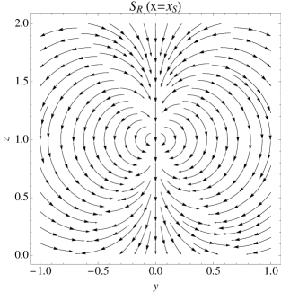
Since ${\bf E}_{M}=0$, we already know from Eq. (37) that there is no outward directed Poynting flux anywhere. Neither the Rindler observer nor the Minkowski observer sees any radiation. For completeness, we write the Rindler Poynting vector explicitly

$$\mathbf{S}=\frac{g_{H}^{2}z^{2}}{4\pi}\left[\gamma_{R}\beta_{R}B_{M}^{\perp}{\bf B}_{M}^{\parallel}-\gamma_{R}^{2}(B_{M}^{\parallel})^{2}{\boldsymbol{\beta}}_{R}\right]$$ (46)

and plot streamlines of $\mathbf{S}$ in Figure 5. Notice there is a component of the Poynting flux parallel to the horizon and there is a component of the Poynting flux into the horizon, both due to the observer’s motion outward.

Figure 5: The $x=x_{S}=0$ slice (plane containing the dipole) of the Poynting flux for the infalling dipole as viewed by Rindler observers. The axes are in units of $Z_{S}$.

For the sake of illustration, we write out the components of ${\bf E}_{R}$ and ${\bf B}_{R}$ from Eq. (43) for the infalling dipole explicitly for the case $\mathbf{m_{S}}=m\mathbf{\hat{e}_{y}}$. Using $\gamma_{R}=\cosh(g_{H}t)$ and $\gamma_{R}\beta_{R}=\sinh(g_{H}t)$ and the magnitude of $r$ from Eq. (44):

$$B_{R}^{x} =\frac{3mxy}{r^{5}}\hbox{cosh}[g_{H}t]$$

$$B_{R}^{y} =-\frac{m\left(r^{2}-3y^{2}\right)}{r^{5}}\hbox{cosh}[g_{H}t]$$

$$B_{R}^{z} =\frac{3my\left(z\hbox{cosh}[g_{H}t]-Z_{S}\right)}{r^{5}}$$

$$E_{R}^{x} =\frac{m\left(r^{2}-3y^{2}\right)}{r^{5}}\hbox{sinh}[g_{H}t]$$

$$E_{R}^{y} =\frac{3mxy}{r^{5}}\hbox{sinh}[g_{H}t]$$

$$E_{R}^{z} =0$$ (47)

Using (IV), we plot the fields, and horizon charge densities and currents at three different times during the infall in Figure 6. As we have already seen from Eqs. (45), there are no charges set up on the horizon and thus no battery. However, there are currents moving in circles along the horizon. These are the currents implied in the discussion surrounding (36) which are responsible for dissipating the energy in the EM fields as they pass through the horizon. Note that the divergence of $\mathbf{\mathcal{J}_{\mathcal{H}}}$ in this case is 0, as can be seen from the purely rotational nature in Figure 6. Recalling Eq. (12), we see that this must be the case for charge conservation to hold in vacuum where currents normal to the horizon, $j_{n}$, must be zero.

$\begin{array}[]{cc}\includegraphics[scale={0.33}]{Infall_Rind_Dipole_BJH_t0.pdf}&\includegraphics[scale={0.33}]{Infall_Rind_Dipole_ESig_t0.pdf}\\ \\ \includegraphics[scale={0.33}]{Infall_Rind_Dipole_BJH_t6gh.pdf}&\includegraphics[scale={0.33}]{Infall_Rind_Dipole_ESig_t6gh.pdf}\\ \\ \includegraphics[scale={0.33}]{Infall_Rind_Dipole_BJH_t12gh.pdf}&\includegraphics[scale={0.33}]{Infall_Rind_Dipole_ESig_t12gh.pdf}\end{array}$

Figure 6: 3D visualization of the magnetic dipole field lines of a dipole falling from initial height $z_{S}(t=0)=Z_{S}$ above the Rindler horizon, denoted by the gray plane at $z=0$. The visualization region is a cube with side length $2Z_{S}$. On the left, magnetic field lines and the corresponding horizon current densities $\mathbf{J_{\mathcal{H}}}$ are plotted. On the right, electric field lines and corresponding charge densities $\sigma_{\mathcal{H}}$ (0 here) are plotted on the stretched horizon located at $z_{H}=0.01Z_{S}$.

The freely-falling worldline provides a helpful test of our solutions, but no power for an electromagnetic circuit. This system would remain dark, unlike the orbit we explore in the next section. (For an actual BH-NS system at separations that probe spatial curvature, a battery may be established even with pure infall. The effect is not captured here in a flat-wall limit.)

V A Boosted, Freely Falling Dipole Solution

As a second test of the solutions, consider a source that stays at constant $Z_{S}$ in Minkowski but is boosted in the $X$, $Y$ plane. Relative to our Rindler observer, the dipole will appear to fall through the horizon but on an arc.

Taking the boost to be at constant velocity in the $X$-direction, as seen by the Minkowski observer, we have

$$r^{\alpha} =\begin{pmatrix}T-T_{S}\\ X-\beta_{S}T_{S}\\ Y\\ Z-Z_{S}\end{pmatrix}$$ (48)

$$V^{\alpha} =\begin{pmatrix}\gamma_{S}\\ \gamma_{S}\beta_{S}\\ 0\\ 0\end{pmatrix}\qquad a^{\alpha}=\begin{pmatrix}0\\ 0\\ 0\\ 0\end{pmatrix}$$

The coordinate $Z_{S}$ is again simply a number, $\beta_{S}$ and $\gamma_{S}=\left(1-\beta^{2}_{S}\right)^{-1/2}$ are also constant. It is important to note that although the Minkowski observer sees the dipole boosted in the $X$-direction at a constant velocity, the Rindler observer sees the dipole slow down in the $x$-direction as it speeds up in the $z$. This is illustrated in Figure 7.

The retarded time can be found in closed form:

$$T_{*}= \gamma^{2}_{S}{(T-\beta_{S}X)}-$$ (49)

$$\gamma_{S}\sqrt{\gamma^{2}_{S}\left({T-\beta_{S}X}\right)^{2}{-T^{2}+X^{2}+Y^{2}+(Z-Z_{S})^{2}}}$$

so that

$$\left(r\cdot V\right)_{*}=-\left[\gamma^{2}_{S}(X-\beta_{S}T)^{2}+Y^{2}+(Z-Z_{S})^{2}\right]^{1/2}$$ (50)

Eq. (24) with $a=0$ and $\mathbf{\dot{m}}=0$ then gives the 4-potential for a boosted Minkowski dipole. From the 4-potential or the field tensor, Minkowski ${\bf E}_{M}$ and ${\bf B}_{M}$ can be derived from Eq. (28) or (27).

Figure 7: Spacetime diagram depicting the $x$-component of the infalling, boosted dipole worldline of §V from the Rindler observer’s perspective, for three different values of $\beta_{S}$. The z-component of the worldline is identical to that portrayed for the infalling dipole in the bottom panel of Figure 4 except the light cone structure is altered. Because the infalling boosted dipole approaches the speed of light in the z-direction, the motion in the x-direction must go to zero ($dx/dt\rightarrow 0$). This is evident from the worldlines in this figure which asymptote to vertical lines.

As a check, we may also derive the electromagnetic fields by writing the field tensor for a dipole in the rest frame of a Minkowski observer, transform to a boosted frame, and then transform to the accelerated Rindler frame.

Let the reference frame of the Minkowski observer at rest with respect to the dipole be denoted by a double prime, the frame of the Minkowski observer boosted relative to the source by a single prime, and the Rindler frame by no prime. Then the field tensor $F^{\alpha^{\prime\prime}\beta^{\prime\prime}}(X^{\mu^{\prime\prime}})$ is constructed from Eq. (42). The field tensor in the Minkowski boosted frame is given by

$$F^{\alpha^{\prime}\beta^{\prime}}(\mathbf{X^{\prime}})=\Lambda^{\alpha^{\prime}}_{\sigma^{\prime\prime}}\Lambda^{\beta^{\prime}}_{\rho^{\prime\prime}}F^{\sigma^{\prime\prime}\rho^{\prime\prime}}(\mathbf{X^{\prime\prime}})$$ (51)

where $\Lambda^{\alpha^{\prime}}_{\sigma^{\prime\prime}}$ is the Lorentz transformation for a boost in the $X$ direction. The boosted coordinates $X^{\mu^{\prime}}$ are given in terms of the rest frame coordinates $X^{\mu^{\prime\prime}}$ via an inverse Lorentz transformation. The Rindler $\bf{E_{R}}$ and $\bf{B_{R}}$ fields are then found via Eq.  (6) and (32),

$$E_{R}^{\alpha}(\bf{x}) =\frac{\partial x^{\alpha}}{\partial x^{\alpha^{\prime}}}F^{\alpha^{\prime}\mu^{\prime}}{(\bf{X^{\prime}})}u^{R}_{\mu^{\prime}}$$

$$B_{R}^{\alpha}(\bf{x}) =\frac{1}{2}\frac{\partial x^{\alpha}}{\partial x^{\alpha^{\prime}}}\epsilon^{\alpha^{\prime}\mu^{\prime}\gamma^{\prime}\delta^{\prime}}F_{\gamma^{\prime}\delta^{\prime}}(\mathbf{X^{\prime}})u^{R}_{\mu^{\prime}}.$$ (52)

where $u^{R}_{\mu^{\prime}}$ are the components of the Rindler observer’s 4-velocity as viewed by the boosted Minkowski observer. The $X^{\mu^{\prime}}(x^{\mu})$ are given by Eqs.  (3) and we have again kept Rindler coordinates lower case while Minkowski coordinates are upper case.

Carrying out the above procedure, we start with an observer co-moving with the dipole. This observer sees fields,

$${\bf E_{M^{\prime\prime}}} =0$$

$${\bf B_{M^{\prime\prime}}} =\frac{3\hat{\bf r}^{\prime\prime}({\bf m_{S}}\cdot\hat{\bf r}^{\prime\prime})-{\bf m_{S}}}{{\bf r}^{\prime\prime\ 3}}$$ (53)

where ${\bf m_{S}}$ is the constant rest-frame value of the dipole’s magnetic moment and ${\bf r}^{\prime\prime}$ is a radial coordinate in the rest-frame of the dipole. There exists another Minkowski observer boosted by $-{\boldsymbol{\beta}}_{S}$ relative to the source who measures the fields

$${\bf E_{M^{\prime}}} =-\gamma_{S}({\boldsymbol{\beta}}_{S}\times{\bf B_{M^{\prime\prime}}})$$

$${\bf B_{M^{\prime}}} ={\bf B_{M^{\prime\prime}}}+(\gamma_{S}-1)\hat{{\boldsymbol{\beta}}}_{S}\times({\bf B_{M^{\prime\prime}}}\times\hat{{\boldsymbol{\beta}}}_{S})$$ (54)

We obtain the Rindler fields by an application of Eq.  (34):

$${\bf E}_{R} =\gamma_{S}\gamma_{R}\left({\boldsymbol{\beta}}_{R}\times\mathbf{B_{M^{\prime\prime}}}\right)$$

$$- \left[\gamma_{S}\hat{{\boldsymbol{\beta}}}_{R}\cdot\left({\boldsymbol{\beta}}_{S}\times\mathbf{B_{M^{\prime\prime}}}\right)\right]\hat{{\boldsymbol{\beta}}}_{R}$$

$$- \left[\gamma_{R}\mathbf{B_{M^{\prime\prime}}}\cdot\left(\left(\gamma_{S}-1\right)|{\boldsymbol{\beta}}_{R}|\hat{{\boldsymbol{\beta}}}_{S}-\gamma_{S}|{\boldsymbol{\beta}}_{S}|\hat{{\boldsymbol{\beta}}}_{R}\right)\right]\left(\hat{{\boldsymbol{\beta}}}_{R}\times\hat{{\boldsymbol{\beta}}}_{S}\right)$$

$${\bf B}_{R} =\gamma_{S}\gamma_{R}\mathbf{B_{M^{\prime\prime}}}$$

$$- \left[\gamma_{S}\left(\gamma_{R}-1\right)\left(\mathbf{B_{M^{\prime\prime}}}\cdot\hat{{\boldsymbol{\beta}}}_{R}\right)\right]\hat{{\boldsymbol{\beta}}}_{R}$$

$$- \left[\gamma_{R}\mathbf{B_{M^{\prime\prime}}}\cdot\left(\left(\gamma_{S}-1\right)\hat{{\boldsymbol{\beta}}}_{S}-\gamma_{S}|{\boldsymbol{\beta}}_{S}|{\boldsymbol{\beta}}_{R}\right)\right]\hat{{\boldsymbol{\beta}}}_{S}$$ (55)

The horizon charge and current densities are

$$\sigma_{\mathcal{H}} \equiv\frac{\bf{E^{\perp}_{R}}}{4\pi}\bigg{|}_{\mathcal{H}}=-\frac{\hat{{\boldsymbol{\beta}}}_{R}\cdot(\gamma_{S}{\boldsymbol{\beta}}_{S}\times\mathbf{B}^{\parallel}_{M^{\prime\prime}})_{z=z_{\mathcal{H}}}}{4\pi}$$

$$\mathbf{\mathcal{J}_{\mathcal{H}}} \equiv\left[\frac{1}{4\pi}\hat{{\boldsymbol{\beta}}}_{R}\times\alpha\mathbf{B_{R}^{||}}\right]_{\mathcal{H}}$$

$$=\gamma_{R}\frac{g_{H}z_{\mathcal{H}}}{4\pi}\left[\gamma_{S}\left(\hat{{\boldsymbol{\beta}}}_{R}\times\mathbf{B}^{\parallel}_{M^{\prime\prime}}\right)\right.$$

$$- \left.\mathbf{B_{M^{\prime\prime}}}\cdot\left(\left(\gamma_{S}-1\right)\hat{{\boldsymbol{\beta}}}_{S}-\gamma_{S}|{\boldsymbol{\beta}}_{S}|{\boldsymbol{\beta}}_{R}\right)\left(\hat{{\boldsymbol{\beta}}}_{R}\times\hat{{\boldsymbol{\beta}}}_{S}\right)\right]_{z=z_{\mathcal{H}}}$$ (56)

This example manifests charge separation and therefore a voltage drop across the event horizon. We have established a BH battery.

To express these Rindler fields in Rindler coordinates, we perform a Lorentz transformation on the Minkowski 4-vector $r^{\prime\prime}$ for a boost in the x-direction and use Eqs. (3) to write,

$${\bf r}^{\prime\prime}=(\gamma_{S}\left(x-\beta_{S}z\hbox{sinh}[g_{H}t]\right),y,z\hbox{cosh}[g_{H}t]-Z_{S}).$$ (57)

Eqs. (57), (53), and (55) then give the Rindler fields in Rindler coordinates.

The Rindler fields derived in this manner agree with the fields derived from inserting (48) into the 4-potential as they must.

Choosing $\mathbf{m_{S}}=m\mathbf{\hat{e}_{y}}$, given that we boost in the x-direction, leads to the simplest form for the observed 4-dipole moment,

$$m_{R}^{\mu}=m_{M^{\prime\prime}}^{\mu}=m_{M^{\prime}}^{\mu}=(0,{\bf m_{S}}).$$ (58)

We write out the components of ${\bf E}_{R}$ and ${\bf B}_{R}$ for the boosted, infalling dipole explicitly:

$$B_{R}^{x} =\gamma_{S}\frac{3my\left(x\hbox{cosh}[g_{H}t]-\beta_{S}Z_{S}\hbox{sinh}[g_{H}t]\right)}{r^{5}}$$

$$B_{R}^{y} =-\gamma_{S}\frac{m\left(r^{2}-3y^{2}\right)}{r^{5}}\hbox{cosh}[g_{H}t]$$

$$B_{R}^{z} =\gamma_{S}\frac{3my\left(z\hbox{cosh}[g_{H}t]-Z_{S}\right)}{r^{5}}$$

$$E_{R}^{x} =\gamma_{S}\frac{m\left(r^{2}-3y^{2}\right)}{r^{5}}\hbox{sinh}[g_{H}t]$$

$$E_{R}^{y} =\gamma_{S}\frac{3my\left\{x\hbox{sinh}[g_{H}t]+\beta_{S}\left(z-Z_{S}\hbox{cosh}[g_{H}t]\right)\right\}}{r^{5}}$$

$$E_{R}^{z} =\gamma_{S}\frac{m\left(r^{2}-3y^{2}\right)}{r^{5}}\beta_{S}$$ (59)

where $r$ is the RHS of (50) in Rindler coordinates. Using the above, we plot the fields, and horizon charge and current densities, given by Eqs.  (56), at three different times during the inspiral in Figure 8.

Figure 9 shows the Poynting flux generated by the above fields for $\beta_{S}=0.1,0.5,0.9$. The Poynting flux is directed into the horizon below the dipole signifying the dissipation of the field energy into the horizon (via ohmic dissipation from horizon currents). The increasingly uniform $z$ component of the Poynting flux for increasing $\beta_{S}$ is due to the increasing disparity between $t$ and $t_{*}$ (observers see further into the relative past of the dipole) for larger $\beta_{S}$ and smaller $z$. There is no observed Poynting flux at infinity in this case and hence no radiation from the moving dipole in vacuum. We elaborate on the above points further in §VII.

$\begin{array}[]{cc}\includegraphics[scale={0.33}]{BoostInfall_Rind_Dipole_BJH_t0.pdf}&\includegraphics[scale={0.33}]{BoostInfall_Rind_Dipole_ESig_t0.pdf}\\ \\ \includegraphics[scale={0.33}]{BoostInfall_Rind_Dipole_BJH_t6gh.pdf}&\includegraphics[scale={0.33}]{BoostInfall_Rind_Dipole_ESig_t6gh.pdf}\\ \\ \includegraphics[scale={0.33}]{BoostInfall_Rind_Dipole_BJH_t12gh.pdf}&\includegraphics[scale={0.33}]{BoostInfall_Rind_Dipole_ESig_t12gh.pdf}\end{array}$

Figure 8: 3D visualization of the field lines of a dipole spiraling into the Rindler horizon from initial height $z_{S}(t=0)=Z_{S}$ with an initial boost of $\beta_{S}=0.9$ in the $x$-direction. The visualization region spans from $-2Z_{S}$ to $2Z_{S}$ in the x- and y-directions and extends $2Z_{S}$ above the Rindler horizon. Surface currents $\mathbf{J_{\mathcal{H}}}$ and surface charge densities $\sigma_{\mathcal{H}}$ are plotted on the stretched horizon located at $z_{H}=0.01Z_{S}$.

Figure 8, as well as the expression for $E_{R}^{z}$ and Eq.  (11) for the horizon charge density, indeed confirm that charge separation occurs on the stretched horizon. Figure 10 explores the horizon charge density further. As we will elaborate in §VII, this charge separation can be considered a result of tangential components of the dipole magnetic field sourcing horizon currents via (11). Because no currents are entering or leaving the horizon in the vacuum case, these horizon currents pile up charge on the horizon, that is the divergence of the horizon current in (12) is not 0, but cancels a time changing charge density. This is why the currents seem to flow towards regions of positive charge in Figure 10. We see also that, as might have been expected, the magnitude of the charge separation grows with the speed of the boost, i.e. the more energy given to boost the dipole along the horizon, the higher the voltage of the horizon battery.

The line of zero charge density in the plane of the stretched horizon is given by,

$$x\big{|}_{\sigma_{\mathcal{H}}=0} =\beta_{S}z_{\mathcal{H}}\hbox{sinh}[g_{H}t]$$

$$\pm\gamma^{-1}_{S}\sqrt{2y^{2}-(z_{\mathcal{H}}\hbox{cosh}[g_{H}t]-Z_{S})^{2}}\ .$$ (60)

On the true horizon,

$$x\big{|}_{\sigma_{H}=0}=\pm\gamma^{-1}_{S}\sqrt{2y^{2}-Z^{2}_{S}}\ .$$ (61)

On the stretched horizon the shape of the charge separation boosts along the horizon at late times, when $z_{\mathcal{H}}\hbox{sinh}[g_{H}t]$ becomes large. On the true horizon however the charge separation is stationary reflecting the freezing in of fields on the horizon.

As can be seen in Figure 10, the $\gamma^{-1}_{S}$ pre-factor in equation (61) morphs the geometry of the charge separation from that of roughly equal parts positive and negative charge at low $\beta_{S}$, to that of smaller regions of larger negative charge density squeezed to the sides of the dipole in the direction of its motion for larger $\beta_{S}$.

The charge separation and corresponding battery emf is a direct consequence of the boosted motion parallel to the horizon. We will see this feature again in the final example (§VII). In the penultimate section §VIII, we estimate the power produced by a black-hole battery, the luminosities attained in the circuit, and the energy scale of the emission.

$\begin{array}[]{c}\includegraphics[scale={0.38}]{FmunuINFBoost_betx01_t01_x0_Syz.pdf}\\ \includegraphics[scale={0.38}]{FmunuINFBoost_betx05_t01_x0_Syz.pdf}\\ \includegraphics[scale={0.38}]{FmunuINFBoost_betx09_t01_x0_Syz.pdf}\end{array}$

Figure 9: An $x=x_{S}=0$ slice of the Poynting flux for the infalling boosted dipole of §V as viewed by Rindler observers for three different boost magnitudes in the $x$-direction, $\beta_{S}=0.1,0.5,0.9$. The Poynting flux is 0 at infinity despite outward components of the field in the region plotted here. The axes are in units of $Z_{S}$.

$\begin{array}[]{c}\includegraphics[scale={0.38}]{INFBoost_betx01_t1_Jxy_SigH_alph1e4.png}\\ \includegraphics[scale={0.38}]{INFBoost_betx05_t1_Jxy_SigH_alph1e4.png}\\ \includegraphics[scale={0.38}]{INFBoost_betx09_t1_Jxy_SigH_alph1e4.png}\end{array}$

Figure 10: Current density vectors (white) overlaid on contours of charge density on the stretched horizon ($\alpha_{\mathcal{H}}=10^{-4}$) of the infalling boosted dipole with rest frame magnetic moment in the $y$-direction. From top to bottom, the magnitude of the boost in the $x$-direction increases from $\beta_{S}=0.1,0.5,0.9$. As inferred from the last of Eqs.  (59), the magnitude of the charge density increases with $\beta_{S}$. Also the shape of the charge separation is squeezed in the direction of source boost as indicated by Eq.  (60). All of the snapshots are taken at $g_{H}t=1$ and the contour labels are arbitrarily scaled. The gray regions are regions of steeply increasing $\sigma_{\mathcal{H}}$ which have been removed to more clearly view the contour structure. The axes are in units of $Z_{S}$.

VI Rindler Dipole

Now suppose there is a magnetic dipole that is uniformly accelerated so that it lives at constant Rindler coordinate $z_{S}$. While the Minkowski observers see this dipole accelerate and asymptote to a null trajectory, the Rindler observers see a source dipole at fixed coordinate distance above the horizon.

This is the first case for which we no longer have a check of our solutions. Nor do we have an obvious alternative method of calculation. We must compute fields from our exact solution for the 4-potential from §III. The kinematics of the accelerated source are characterized by

$$r^{\mu} =\begin{pmatrix}T-T_{S}\\ X\\ Y\\ Z-Z_{S}(T_{S})\end{pmatrix}\qquad V^{\mu}=\gamma_{S}\begin{pmatrix}1\\ 0\\ 0\\ \beta_{S}\end{pmatrix}$$

$$a^{\mu} =\frac{\gamma^{2}_{S}}{Z_{S}}\begin{pmatrix}\beta_{S}\\ 0\\ 0\\ 1\end{pmatrix}\quad\dot{a}^{\mu}=\frac{\gamma^{3}_{S}}{Z^{2}_{S}}\begin{pmatrix}1\\ 0\\ 0\\ \beta_{S}\end{pmatrix}$$

where, in this case, $\beta_{S}=\tanh(g_{H}t_{S})=T_{S}/Z_{S}$, $\gamma_{S}=\cosh(g_{H}t_{S})=(1-(T_{S}/Z_{S})^{2})^{-1/2}$, and $Z_{S}=\sqrt{z^{2}_{S}+T^{2}_{S}}=z_{S}\hbox{cosh}[g_{H}t_{S}]$, where $z_{S}$ is the constant height of the Rindler dipole above the horizon.

Here, the light cone condition is easier to solve in Rindler coordinates. Evaluating the source at the retarded time, $t_{S}=t_{*}$, the light cone condition is

$$x^{2}+y^{2}+z^{2}+z^{2}_{S}-2zz_{S}\hbox{cosh}\left[g_{H}(t-t_{*})\right]=0.$$ (62)

For $z_{S}=$constant, we find

$$t_{*}(x)=t-g_{H}^{-1}\cosh^{-1}\left(\frac{x^{2}+y^{2}+z^{2}+z^{2}_{S}}{2zz_{S}}\right)$$ (63)

and $T_{*}=z_{S}\sinh(g_{H}t_{*})$.

Now that we have an expression for the retarded time, we can find the fields for our Rindler observer following the prescription of §III. For the sake of illustration, we write the Rindler fields for the specific case where $\mathbf{m_{S}}=m\mathbf{\hat{e}_{y}}$:

$$B_{R}^{x}= -\frac{48mxyzz^{2}_{S}}{\left(r_{-}r_{+}\right)^{5}}\left[r^{2}_{+}-2zz_{S}\right]$$

$$B_{R}^{y}= \frac{8mzz^{2}_{S}}{\left(r_{-}r_{+}\right)^{3}}+B_{R}^{x}\frac{y}{x}$$

$$B_{R}^{z}= \frac{16myz^{2}_{S}}{\left(r_{-}r_{+}\right)^{5}}\left[(r_{-}r_{+})^{2}+6z^{2}z^{2}_{S}\right]+B_{R}^{x}\frac{z}{x}$$

$$\mathbf{E_{R}}= 0$$ (64)

$$r_{\pm} =\sqrt{x^{2}+y^{2}+(z\pm z_{S})^{2}}$$

We plot the above fields in Figure 11 from 4 different points of view; looking down each coordinate axis and looking from a position half way between the $x$ and $y$ axes. From the above expressions we see that even though the Minkowski dipole is accelerated, Rindler observers see no radiation field, nor do they see any electric field at all. This is surprising since the Minkowski observers see a Poynting flux as well as radiation. However, from the expression for the Rindler Poynting flux in terms of Minkowski fields (37), we see that the purely Minkowski term $\left[{\bf E}_{M}^{\parallel}\times{\bf B}_{M}^{\parallel}\right]$ is exactly balanced by terms due to accelerations of the Rindler observers, which account for field energy moving past them as they accelerate. Note that this is also consistent with our choice of the rest frame moments ${\bf{m_{S}}}$ and ${\bf{p_{S}}}$.

As can be seen in Figure 11, at the horizon, the fields align themselves perpendicular to the horizon, i.e ${\bf B}_{\mathcal{H}}=0$. This is a consequence of the conductor-like properties of the horizon, Eqs. (11), along with the ingoing wave boundary conditions, ${\bf B}_{\mathcal{H}}=-\hat{e}_{z}\times{\bf E}_{\mathcal{H}}$ and ${\bf E}_{\mathcal{H}}=\hat{e}_{z}\times{\bf B}_{\mathcal{H}}$ which are a result of choosing stationary observers to measure the fields.

Since ${\bf E}_{R}=0$, no battery is established for the Rindler dipole. But then, no battery would be expected from this configuration given that the dipole is fixed relative to the horizon. When we introduce relative motion, as we do in the next section, we will once again see a power source generated in the form of an event-horizon battery.

$\begin{array}[]{cc}\includegraphics[scale={0.3}]{Stationary_Rindler_Dipole_xy45.png}&\includegraphics[scale={0.3}]{Stationary_Rindler_Dipole_x.png}\\ \includegraphics[scale={0.3}]{Stationary_Rindler_Dipole_y.png}&\includegraphics[scale={0.3}]{Stationary_Rindler_Dipole_z.png}\end{array}$

Figure 11: 3D visualization of the magnetic dipole field lines hovering at constant height $z_{S}$ above the Rindler horizon, denoted by the gray plane at $z=0$. The visualization region is a cube with side length $2z_{S}$.

VII Rindler Dipole Boosted Parallel to the Horizon

We would like to imagine a worldline for the source dipole that mimics a magnetized NS in orbit around a BH. The physical motion we want to represent is best imitated by a source dipole at some fixed Rindler height above the horizon $z_{S}$, but moving parallel to the horizon with some fixed Rindler velocity, $v_{S,x}=$constant, so that

$$x_{S}=v_{S,x}\alpha_{S}t_{S}\ .$$ (65)

The kinematic ingredients are then expressed in Minkowski coordinates as

$$r^{\mu} =\begin{pmatrix}T-T_{S}\\ X-X_{S}(T_{S})\\ Y\\ Z-Z_{S}(T_{S})\end{pmatrix}\qquad V^{\mu}=\gamma_{S}\begin{pmatrix}1\\ \beta_{S,X}\\ 0\\ \beta_{S,Z}\end{pmatrix}$$

$$a^{\mu} =\frac{\gamma^{2}_{S}}{Z_{S}}\begin{pmatrix}\beta_{S,Z}\\ 0\\ 0\\ 1\end{pmatrix}\qquad\dot{a}^{\mu}=\frac{\gamma^{3}_{S}}{Z^{2}_{S}}\begin{pmatrix}1\\ 0\\ 0\\ \beta_{S,Z}\end{pmatrix}$$

Here $\gamma_{S}$ is the total Lorentz factor computed with ${\boldsymbol{\beta}}_{S}=\beta_{S,X}{\bf{e_{X}}}+\beta_{S,Z}{\bf{e_{Z}}}$ and

$$\beta_{S,X} ={v_{S,x}}\frac{z_{S}}{Z_{S}}$$

$$\beta_{S,Z} =\frac{T_{S}}{Z_{S}}$$ (66)

and again $Z_{S}=\sqrt{z^{2}_{S}+T^{2}_{S}}=z_{S}\hbox{cosh}[g_{H}t_{S}]$, with $z_{S}$ the constant height of the Rindler dipole above the horizon. Notice that as long as $|v_{S,x}|\leq 1$, the source will travel slower than the speed of light at all times, $\beta_{S}\leq 1$.

Figure 12: Spacetime diagram in the Rindler frame depicting the worldline of a source boosted parallel to the Rindler horizon (§VII). The light ray (dotted line) has slope $dt/dz=(g_{H}z_{S})^{-1}$ and the worldline has slope $(v_{S,x}g_{H}z_{S})^{-1}$, where $z_{S}$ is the constant position of the source above the Rindler horizon.

The light-cone condition in Rindler coordinates can no longer be found in closed form for $t_{S}=t_{*}$. We can however write $A^{\alpha}$ or $F^{\alpha\beta}$ in terms of $t_{*}$ (or $T_{*}$) and solve numerically for the retarded time. It is extremely helpful that we never have to take explicit derivatives of $t_{*}$ since the first relation in Eq. (23) allows us to re-express derivatives in terms of more transparent variables.

Figure 13 plots the fields of a parallel-boosted dipole for the choice of a magnetic dipole moment in the $y$-direction and a boost in the $x$-direction. Each panel plots streamlines of the magnetic (blue) or electric (red) fields in the $y-z$ plane containing the source. Also plotted are contours of $B^{x}_{R}/\sqrt{(B^{y}_{R})^{2}+(B^{z}_{R})^{2}}$ or $E^{x}_{R}/\sqrt{(E^{y}_{R})^{2}+(E^{z}_{R})^{2}}$ to give a sense of the 3D nature of the fields. Successive rows correspond to increases in $v_{S,x}$. The fields do not evolve in time except for their constant (universal-time) velocity motion in the $x$-direction.

The dipolar magnetic field structure flattens near the horizon due to time dilation. Observers below the dipole source see the dipole as it was further in the past, when the dipole was further away in the negative $x$-direction, than do observers the same distance above the source. This leads to an overall dragging of field lines along the horizon as explained in more detail in the figure captions.

We also see this effect in Figure 16 which is a slice of the Poynting-flux vector field in the $y-z$ plane containing the source. For large $v_{S,x}$, observers at small $z$ see fields from when the dipole is relatively far away and thus do not see the dipole structure of the field energy flowing past them, only nearly uniform $z$ and $y$-components.

$\begin{array}[]{c}\includegraphics[scale={0.33}]{FmunuBoost_StrmCont_betx01_t1_xvat_EByz.png}\\ \includegraphics[scale={0.33}]{FmunuBoost_StrmCont_betx05_t1_xvat_EByz.png}\\ \includegraphics[scale={0.33}]{FmunuBoost_StrmCont_betx09_t1_xvat_EByz.png}\end{array}$

Figure 13: Streamlines of the magnetic (left) and electric (right) fields in the plane $x=0$ for a magnetic dipole with dipole moment ${\bf m}\propto\hat{\bf e}_{y}$ and with three different boost velocities increasing from top to bottom $v_{S,x}=0.1,0.5,0.9$ in the $x$-direction. Plotted over the streamlines are contours of the x-components of the fields relative to the $y-z$ magnitude. Darker regions represent negative values and lighter regions represent positive values. The white regions are clipped to better view the contour structure. The snapshots here are taken at $g_{H}t=1/4$, however the fields retain the same structure for all time except for their motion in the x-direction (out of the page). The axes are in units of $z_{S}$. Since the source is boosted, observers near the horizon see the fields as they would have been when the dipole was further away in the negative x-direction. The result is an observed dragging of the fields along the horizon in the negative x-direction. The observed larger radius of curvature of the dipole lobes manifests itself as the flattening of the field lines. As can be gathered from Figure 12, this effect is intensified for larger boost factor $v_{S,x}$. In the $v_{S,x}=0.9$ case, plotted at the bottom of the figure, the 2D slice of the magnetic field loses its dipolar structure in most of the region below the source. As $v_{S,x}$ approaches $1$, the slope of the source worldline approaches the light cone slope and an observer at a given $z$ will see further and further into the relative past of the dipole. Note also that the contours in the left panels show that the circulation direction of the dipole lobes changes sign at a value of $z$ which gets larger for larger $v_{S,x}$. This change in sign results since observers near the horizon see fields from further in the past when the fields were pointing in a different x-direction. The increase in z-location of this turning point for larger $v_{S,x}$ can again be understood from Figure 12.

For small $v_{S,x}$, the fields resemble those in the stationary case, threading the horizon nearly perpendicularly. As $v_{S,x}$ is increased, the dragging effect causes the fields near the horizon to lay down tangentially to the horizon as the source moves along. Figure 14 shows a 3D representation of the dragging effect for the $v_{S,x}=0.2$ case. In the left panel of Figure 14 we see that the tangential magnetic fields source horizon currents. Via horizon charge conservation, these currents build up horizon charge density which we observe in the right panel of Figure 14 and interpret as the normal components of the induced electric fields. Figure 15 shows the horizon charge and current densities for three different $v_{S,x}$, all at $g_{H}t=10$. As time progresses, these same charge and current distributions are dragged behind the dipole on the stretched horizon at a lag distance which increases as $v_{S,x}$ increases, and also as the distance between the stretched and true horizons decreases.

$\begin{array}[]{cc}\includegraphics[scale={0.34}]{Boost_BandJH_t004_beta02_sqr_view.pdf}&\includegraphics[scale={0.34}]{Boost_EandSigH_t004_beta02_sqr_view.pdf}\end{array}$

Figure 14: A 3D visualization of the magnetic fields lines and corresponding horizon currents $\mathbf{J_{\mathcal{H}}}$ (left) and electric field lines with the corresponding horizon charges $\sigma_{\mathcal{H}}$ (right) for the boosted Rindler dipole. The case shown is for $v_{S,x}=0.2$.

An interpretation of this behavior follows similarly to that of (MacDonald and Suen, 1985) for the case of an electric point-charge boosted parallel to the Rindler horizon. In the electric point-charge case, the charge distribution induced on the horizon is also dragged behind the boosted source. Via charge conservation, this necessitates horizon currents to redistribute charges. Such horizon currents can be thought of as due to tangential components of magnetic fields induced by the moving point-charge.

$\begin{array}[]{c}\includegraphics[scale={0.35}]{Boost_betx01_t10_Jxy_SigH_alph1e4.png}\\ \includegraphics[scale={0.35}]{Boost_betx05_t10_Jxy_SigH_alph1e4.png}\\ \includegraphics[scale={0.35}]{Streams_Boost_betx09_t10_Jxy_SigH_alph1e4.png}\end{array}$

Figure 15: An identical plot to Figure 10 but for the boosted case. Current density vectors (white) are overlaid on contours of charge density on the stretched horizon ($\alpha_{\mathcal{H}}=10^{-4}$) of the boosted dipole with magnetic moment in the $y$-direction. The bottom panel also plots streamlines of the currents. From top to bottom, the magnitude of the boost in the $x$-direction increases from $v_{S,x}=0.1,0.5,0.9$. Each snapshot is taken at $g_{H}t=10$. The configuration drags along the stretched horizon keeping a constant lag distance behind the moving source. The induced currents can be thought of as redistributing charge in order to slide the charge distribution along behind the boosted dipole. The gray regions are regions of steeply increasing $\sigma_{\mathcal{H}}$ which have been removed to more clearly view the contour structure. The axes are in units of $z_{S}$.

The key result from this example is the explicit charge separation and therefore voltage drop across the event horizon. We have established an event-horizon battery, a power source for a BH-NS electromagnetic circuit. The boosted Rindler dipole provides a proxy for a NS in orbit around a big BH. We will use this case to estimate some astrophysically relevant scales in the following section.

$\begin{array}[]{c}\includegraphics[scale={0.38}]{FmunuBoost_betx01_t01_x0_Syz.pdf}\\ \includegraphics[scale={0.38}]{FmunuBoost_betx05_t01_x0_Syz.pdf}\\ \includegraphics[scale={0.38}]{FmunuBoost_betx09_t01_x0_Syz.pdf}\end{array}$

Figure 16: An $x=x_{S}=0$ slice through the Poynting flux. The plane contains the source as viewed by Rindler observers for three different boost magnitudes in the $x$-direction, $v_{S,x}=0.1,0.5,0.9$. The Poynting flux is 0 at infinity despite outward components of the field in the region plotted here. The axes are in units of $z_{S}$.

VIII Consequences for the BH-NS Binary

VIII.1 Voltage, Luminosity, and Energy

We utilize the electromagnetic field solutions of the boosted, Rindler dipole of §VII to estimate the power output and maximum energy of radiation a BH battery can supply. We treat the BH-NS system as a series circuit containing resistors and a battery with voltage given via (13) from the electromagnetic field solutions. For simplicity, we imagine sticking one wire of the circuit into the point of maximum horizon potential, and the other wire, a distance of $2M$ away in the y-direction. From (10), this separation can be compared to to a circuit connecting the pole and equator of a Schwarzschild BH. (Although this seems arbitrary, there is little dependence on the distance. We could have stuck the other wire at infinity with little difference in results.) For the boosted Rindler dipole solutions with $\mathbf{m_{S}}=m\mathbf{e_{y}}$, the y-component of the vector potential vanishes. Then from the potential of Eq. (13) and the electric field Eq. (28) in a Rindler coordinate frame, we have $\nabla_{y}V_{\mathcal{H}}=\alpha E^{R}_{y}=\alpha^{2}\nabla_{y}A^{0}_{R}$, and therefore $V_{\mathcal{H}}=\alpha^{2}A_{R}^{0}$ across regions of charge separation estimates the voltage drop on the horizon. In terms of the Rindler retarded time, and with physical constants restored, the horizon voltage is,

$$V_{\mathcal{H}} =\frac{c^{2}v_{S,x}z_{H}m}{8GM}\left(v^{2}_{S,x}z_{S}\frac{g_{H}}{c}t_{*}-v_{S,x}x+z_{H}\mathcal{\tilde{S}}\right)^{-3}\times$$ (67)

$$\left[z_{H}\left(1+2v^{2}_{S,x}+\mathcal{\tilde{C}}2\right)+2v_{S,x}\mathcal{\tilde{S}}\left(x-v_{S,x}z_{S}\frac{g_{H}}{c}t_{*}\right)-2\mathcal{\tilde{C}}\left(\frac{x^{2}+v^{2}_{S,x}z^{2}_{S}+z^{2}_{H}}{z_{S}}+v_{S,x}\frac{g_{H}}{c}t_{*}\left(v_{S,x}z_{S}\frac{g_{H}}{c}t_{*}-2x\right)\right)\right]$$

$${\rm with}$$

$$\mathcal{\tilde{C}} =\cosh{\left[\frac{g_{H}}{c}(t-t_{*})\right]},\qquad\mathcal{\tilde{S}}=\sinh{\left[\frac{g_{H}}{c}(t-t_{*})\right]},\qquad\mathcal{\tilde{C}}2=\cosh{\left[2\frac{g_{H}}{c}(t-t_{*})\right]}$$

where $m$ is the NS rest frame dipole moment (See (68)) and the retarded time $t_{*}$ is a function of the (Rindler) observer coordinates.

We compute power radiated by such a circuit from (14). To do so, we estimate the physically relevant values of the various parameters. Very near the Schwarzschild horizon, in physical units, the gravitational acceleration is

$$g_{H} =\frac{c^{4}}{4GM}\simeq 1.5\times 10^{14}\left(\frac{10M_{\odot}}{M}\right)\frac{\rm{cm}}{\rm{s}^{2}}$$

about 100 billion times that on Earth for a $10M_{\odot}$ black hole. The magnitude of the NS’s magnetic dipole moment written in terms of the magnetic field strength at the NS’s poles $B_{p}$ and the radius of the NS $R_{NS}$ is of order,

$$m =\frac{B_{p}R^{3}_{NS}}{2}\simeq 5\times 10^{29}\left(\frac{B_{p}}{10^{12}G}\right)\left(\frac{R_{NS}}{10^{6}cm}\right)^{3}\rm{G}\ \rm{cm}^{3}\ .$$ (68)

We must also approximate the resistances in our astrophysical circuit diagramed in Figure 1. We have three resistors to consider: the horizon with resistance $\mathcal{R}_{H}$, the NS crust with resistance $\mathcal{R}_{NS}$ and the plasma of the NS magnetosphere denoted by $\mathcal{R}_{\rm{plasma}}$. The horizon resistance is known from the membrane paradigm to be Thorne et al. (1986)

$$\mathcal{R}_{H}\simeq\frac{4\pi}{c}=4.2\times 10^{-10}\rm{s}\ \rm{cm}^{-1}=377\Omega\ \ .$$ (69)

The resistivity of the NS crust is likely very small compared to $\mathcal{R}_{H}$, on the order of $10^{-24}s^{-1}$ (see e.g. (Piro, 2012)); thus we set $\mathcal{R}_{NS}=0$.

The value of $\mathcal{R}_{\rm{plasma}}$ is an interesting unknown and requires numerical exploration beyond the scope of this article. For our present purposes, as a rough guide, we choose an effective value of $\mathcal{R}_{\rm{plasma}}=\mathcal{R}_{H}/2$, because it gives maximum power output through $\mathcal{R}_{\rm{plasma}}$. Ref. McWilliams and Levin (2011) choose $\mathcal{R}_{\rm{plasma}}$ based on equating the power dissipated due to curvature radiation with the power dissipated due to ohmic dissipation $I^{2}\mathcal{R}_{\rm{plasma}}$. Upon solving for $\mathcal{R}_{\rm{plasma}}$, they find $\mathcal{R}_{\rm{plasma}}=\mathcal{R}_{H}$ when the plasma velocity is $\sim 0.7c$. However, the estimate is sensitive to the plasma particle velocity. The dependence of power output on $\mathcal{R}_{\rm{plasma}}$ for a similar NS-NS circuit with non-zero $\mathcal{R}_{NS}$ is explored in Piro (2012), however the NS-BH case is simpler since the denominator of the power formula (14) is dominated by $\mathcal{R}_{H}$.

Since we have set the NS resistance to 0, we focus on the power radiated in the space between the NS and BH, i.e. $\mathcal{R}_{i}=\mathcal{R}_{\rm{plasma}}$ in (14). Since the horizon potential is symmetric around the line $y=y_{S}$, which contains the maximum of the potential and thus one of the circuit wires, we multiply the above luminosity by a factor of 2. The combination of our choices for $\mathcal{R}_{H}$ and $V_{\mathcal{H}}$ will correspond to maximum achievable bolometric luminosities when $\mathcal{R}_{NS}$ is ignored.

The circuit is connected if the BH is within the light cylinder of the NS:

$$R_{lc} =\frac{c}{\Omega_{NS}}=5\times 10^{9}\left(\frac{P}{1s}\right)\ \rm{cm}$$

$$\sim 3\times 10^{3}\left(\frac{P}{1s}\right)\left(\frac{10M_{\odot}}{M}\right)\frac{GM}{c^{2}}$$ (70)

where $P$ is the period of the NS spin and in the last line we quote the radius in units of $M$. We choose a fiducial horizon distance of $z_{S}=3GM/c^{2}$ where the Rindler limit is valid and the pair has approached extremely close prior to merger. For BH’s with $M\gtrsim 10^{4}M_{\odot}$ our fiducial value of $z_{S}$ is larger than the light cylinder of the NS and the pair is unplugged. We address the case for these larger black holes in the next section. For lighter BHs, the circuit will connect when the NS is a distance above the horizon $\sim R_{lc}$ and the power supplied will grow until it reaches a maximum around our fiducial distance $z_{s}=3GM/c^{2}$ just prior to merger. Realistically, the compact objects will plunge extremely rapidly at such close separations so we only use these values to get a sense of the maximum blast of luminosity. For a $10M_{\odot}$ BH, $R_{lc}\gg z_{S}$ and so the circuit is connected for many orbits before maximum is reached.

The maximum horizon voltage and corresponding luminosities are plotted for $10M_{\odot}$, $10^{2}M_{\odot}$, and $10^{3}M_{\odot}$ BH’s in Figure 17 for $v_{S,x}$ varying from $0.01$ to $0.95$. For comparison, $v_{S,x}\sim 0.5$ at the last stable circular Schwarzschild orbit.

Finally then we have our answer. We estimate the voltage of our BH battery to be $\sim 10^{16}$ statvolts for a $10M_{\odot}$ BH, $\sim 10^{14}$ statvolts for a $10^{2}M_{\odot}$ BH, and $\sim 10^{12}$ statvolts for a $10^{3}M_{\odot}$ BH when $v_{S,x}\sim 0.5$. The luminosities in this limited approximation are $\sim 10^{42}$ erg/s, $10^{38}$ erg/s, and $10^{34}$ erg/s respectively.

As is suggested by the pre-factor in (67), the horizon voltage and the luminosity decrease with increasing BH mass. For $z_{S}\rightarrow 0$, the horizon voltage scales as $M^{-1}$ and the luminosity as $M^{-2}$. Otherwise, terms proportional to $g_{H}$ inside the brackets in Eq.  (67) dominate and thus the voltage goes as $M^{-2}$ causing the luminosity to scale as $M^{-4}$. Comparison of the three panels of Figure 17 confirms this scaling with BH mass.

This scaling also agrees with (McWilliams and Levin, 2011) where the BHNS battery was first proposed. In (McWilliams and Levin, 2011) the physical mechanism was sketched out in a non-relativistic calculation. The analytic, relativistic solutions obtained here are in agreement with the findings of (McWilliams and Levin, 2011). Specifically, (McWilliams and Levin, 2011)’s Eq.  (6) for $\mathcal{L}$ exhibits the same scaling with black hole mass and NS magnetic field strength as does our Eq.  (1). Also, (McWilliams and Levin, 2011)’s Eq.  (6) is calculated for similar parameters that we use in our calculation. They choose $\mathcal{R}_{\rm plasma}=\mathcal{R}_{\rm H},\mathcal{R}_{NS}=0$, $B_{p}=10^{12}$, $M=10M_{\odot}$, and a separation corresponding to the NS orbiting at the light ring of a Schwarzschild BH. Hence we may also compare magnitudes of the computed luminosities in each study, and we find that they agree in order of magnitude. Note that the inverse BH mass dependence arises because we are comparing luminosities for different BH masses while holding the distance of the dipole source from the horizon at a fixed number of gravitational radii (which scales with $M$).

$\begin{array}[]{c}\includegraphics[scale={0.3}]{LOG10_Lum_Volt_M1_zs3M_vsx_Rp02_zh1en4.pdf}\\ \includegraphics[scale={0.3}]{LOG10_Lum_Volt_M2_zs3M_vsx_Rp02_zh1en4.pdf}\\ \includegraphics[scale={0.3}]{LOG10_Lum_Volt_M3_zs3M_vsx_Rp02_zh1en4.pdf}\end{array}$

Figure 17: Log-luminosity computed from Eq. (14) (blue, solid line and leftmost y-axis labels) and representative log-voltage drop on the horizon (red, dashed line and rightmost y-axis labels). Luminosities and voltages are computed for $M=10M_{\odot},10^{2}M_{\odot}$, and $10^{3}M_{\odot}$ with the dipole at Rindler height $z_{S}=3M$ as a function of $v_{S,x}$ varying from $0.01$ to $0.95$. The last stable circular orbit in the Schwarzschild spacetime would have $v_{S,x}=0.5$.

We can also compute the maximum energy given to magnetosphere particles by the horizon battery. To be clear, we are not calculating the spectrum – which promises to be complicated – just the maximum energy scale. The magnitude of horizon voltages plotted in Figure 17 makes evident that the highest energy particles accelerated via the horizon battery will radiate their energy via curvature radiation. A Rindler observer at the instantaneous location of an accelerating plasma particle will measure a local energy given by the characteristic energy of curvature radiation,

$$\epsilon_{R}=\frac{3hc}{4\pi}\frac{\gamma^{3}_{p}}{\eta R_{LC}}$$ (71)

where $h$ is Planck’s constant, $\gamma_{p}$ is the Lorentz factor of the plasma particle (electron or positron) measured by a Rindler observer, and we have parameterized the radius of curvature of a magnetic field line by a constant $\eta$ times the NS light cylinder radius. We choose $\eta=0.1$ throughout. The energy measured by an observer at infinity is found by multiplying by a factor of $\alpha=(g_{H}/c^{2})z=(4GM/c^{2})^{-1}z$, which accounts for the gravitational redshift, which is to be evaluated at the Rindler $z$ coordinate of emission.

$$\epsilon_{\infty}=\alpha\frac{3hc}{4\pi}\frac{\gamma^{3}_{p}}{\eta R_{LC}}$$ (72)

Keep in mind however, that far enough from the horizon, where the Rindler limit to the Schwarzschild spacetime breaks down ($\alpha\gtrsim 1$), Rindler-$\alpha$ does not predict the correct gravitational redshift. So, we can only use Eq. (72) for emission that originates close to the horizon, consistent with the regime in which we are working.

We next solve for the values of $\gamma_{p}$. For a given BH mass and horizon distance $z_{S}$ as a function of dipole boost $v_{S,x}$, we estimate the maximum $\gamma_{p}$ in the radiation reaction limit, in which the rate of energy gain from the horizon battery is balanced by the rate of energy loss due to curvature radiation.

A Rindler observer at the instantaneous location of an accelerating plasma particle will measure the following energy per unit proper time being radiated from the particle due to dipole radiation,

$$\mathcal{P}=\frac{d\epsilon_{R}}{d\tau_{R}}=\frac{2}{3}e^{2}c\frac{\gamma^{4}_{p}}{(\eta R_{LC})^{2}}.$$ (73)

Eq.  (73) is the standard relativistic Larmor formula for the power.

Then for a plasma particle moving on the path $\mathbf{s}(t)$, the radiation reaction limited $\gamma_{p}$ is given by,

$$e\frac{dV}{ds^{i}}\frac{ds^{i}}{d\tau_{R}}=\frac{2}{3}e^{2}c\frac{\gamma^{4}_{p}}{(\eta R_{LC})^{2}},$$ (74)

where use of the locally observed potential, $V=V_{\mathcal{H}}/\alpha$, is justified since we are only considering an infinitesimal potential difference, not a global value.

Upon inspection of the currents in Figure 15, it is apparent that representatively large horizon electric fields exist at $y=0$ in the $\pm x$ direction. Thus we choose $\mathbf{ds}=dx\mathbf{e_{\hat{x}}}$ which allows us to write

$$|E^{x}_{R}|\left(1-\frac{1}{\gamma^{2}_{p}}\right)^{1/2}=\frac{2}{3}e\frac{\gamma^{4}_{p}}{(\eta R_{LC})^{2}}$$ (75)

where we have written the 3-velocity of the particle (assumed to be only in the x direction) in terms of $\gamma_{p}$. Note that it is $E^{x}_{R}$ and not $\alpha E^{x}_{R}$ which should be on the LHS of (75) because $qE^{x}_{R}$ is the rate of change of momentum as viewed by Rindler observers and we are asking the Rindler observer to locally balance the competing sources of momentum loss and gain.

Solving the above equation for $\gamma_{p}$ then gives the radiation reaction limited Lorentz factor, as observed by Rindler observers, as a function of time. Since, however, the fields are stationary in the frame which drags along with the horizon charges, we need only find the maximum $\gamma_{p}$ at any time and choose that as our fiducial maximum $\gamma_{p}$. Substituting this into (72) and evaluating $\alpha$ at the same $z$ position as we evaluated (75), gives the maximum energy due to curvature radiation that the horizon battery can produce at a given $z_{S}$, $v_{S,x}$, and $M$, according to observers at infinity. In practice we find the largest values of $\epsilon_{\infty}$ when evaluating (75) and (72) at the stretched horizon, although varying the point of evaluation from $z=z_{H}$ up to $z=4M$ changes the result for $\epsilon_{\infty}$ by less than an order of magnitude. Figure 18 plots the maximum $\gamma_{p}$ and $\epsilon_{\infty}$ as a function of $v_{S,x}$ at dipole height of $z_{S}=3GM/c^{2}$ for BH masses $M=10M_{\odot},10^{2}M_{\odot}$, and $10^{3}M_{\odot}$.

We estimate maximum $\gamma_{p}$’s of our BH battery to be $\sim 10^{10.2}$ for a $10M_{\odot}$ BH, $\sim 10^{9.5}$ for a $10^{2}M_{\odot}$ BH, and $\sim 10^{8.7}$ for a $10^{3}M_{\odot}$ BH when $v_{S,x}\sim 0.5$. However, recall that these are the Lorentz factors measured by the Rindler observers at the stretched horizon and do not correspond to the tremendous energies which (71) would imply. It is the energy measured at infinity given by (72) which carries the only physical relevance here. These $\gamma_{p}$’s correspond to maximum curvature radiation energies at infinity of approximately $30$ TeV, $100$ GeV, and $1$ GeV respectively at $v_{S,x}=0.5$. Because of the decrease in horizon voltage for larger mass BH’s, as for the luminosity, the curvature radiation energies are smaller for larger mass BH’s.

We reiterate that the radiation energies plotted here represent the highest energies of radiation that could be emitted by the NS-BH circuit. Firstly this is because we are not accounting for any plasma effects which may act to screen the maximum fields quoted here. In addition to this, we are using the radiation reaction limited $\gamma_{p}$ computed for plasma particles with velocities aligned with the largest values of the electric field across the horizon. There will also be a spectrum of lower energy synchro-curvature radiation not calculated here.

Although we have not computed timescales or detailed spectra of emission we note that with luminosities reaching up to $10^{42}$ erg/s ($10^{48}$ erg/s for magnetars) and with the capability of producing photons with energies reaching into the TeV range, the mechanism discussed here for a BH mass of $10M_{\odot}$ could be capable of producing bursts of gamma-rays. Further investigation of this mechanism and the timescale, as well as any variability, of emission is needed in order to say whether the BH-NS circuit is responsible for previously detected high-energy bursts, or rather, if it is responsible for an as of yet unobserved phenomenon.

We now look closer at the larger BH case, where the Rindler limit is an even better proxy for the physical situation.

$\begin{array}[]{c}\includegraphics[scale={0.3}]{LOG10_noalphEGam_Enrgy_M1_zs3M_vsx.pdf}\\ \includegraphics[scale={0.3}]{LOG10_noalphEGam_Enrgy_M2_zs3M_vsx.pdf}\\ \includegraphics[scale={0.3}]{LOG10_noalphEGam_Enrgy_M3_zs3M_vsx.pdf}\end{array}$

Figure 18: Maximum curvature radiation energies computed from Eq. (72) (blue, solid line and leftmost y-axis labels) and corresponding maximum $\gamma_{p}$ (Eq. 75) to which electrons/positrons can be accelerated (red, dashed line and rightmost y-axis labels). Both are computed for $M=10M_{\odot},10^{2}M_{\odot}$, and $10^{3}M_{\odot}$ with the dipole at Rindler height $z_{S}=3M$ as a function of $v_{S,x}$ varying from $0.01$ to $0.95$.

VIII.2 NS plummet into a SMBH

Although motivated by an interest in stellar mass BHs, the solutions we have found in the Rindler limit well approximate the end of a NS’s plummet into an intermediate mass or super-massive black hole (IMBH, SMBH). We have included analysis for IMBH’s in the previous section, here we consider a SMBH. Recall that for the mechanism to operate, the BH horizon must be within the magnetosphere of the NS; the distance of the NS from the horizon must be less than the light cylinder radius (70) of the NS. In the previous subsection we always had that $R_{lc}\geq z_{S}=3M$. For the SMBH case however, the NS light cylinder is smaller than $3M$. Thus we locate the dipole at $z_{s}=R_{lc}$ so that the circuit is connected. In this case the Rindler approximation is good for the entire time that luminosity can be generated by the BH battery.

In Figure 19, we plot the luminosities and energy of curvature radiation that could be generated by the dipole at a distance $R_{lc}$ from a $10^{6}M_{\odot}$ BH horizon. We find that for $v_{S,x}=0.5$, luminosities of order $10^{26}$ erg/s can be achieved by the SMBH-NS circuit. The maximum $\gamma_{p}$’s are still rather large reaching values of $\sim 10^{7.4}$ at $v_{S,x}=0.5$. However, recall that these are the maximum $\gamma_{p}$’s as measured by Rindler observers at the stretched horizon and so observed energies at infinity are reduced by a factor of $\alpha_{\mathcal{H}}=10^{-4}$ from what would be inferred from $\gamma_{p}$ alone. For $v_{S,x}=0.5$ the SMBH-NS circuit could generate energies of curvature radiation peaking in the X-ray at $\sim 100$ keV.

At luminosities of $\sim 10^{26}$ erg/s and peak radiation energies of $\sim 100$ keV, even if the SMBH were in our own Galactic Center, this signal would be difficult to detect, as it emanates from a noisy galactic nucleus and could be beamed in a direction not guaranteed to intersect Earth. Note however, that in the optimal case of a magnetar with $B_{p}\simeq 10^{15}G$, and a slower spin period of $\sim 10s$, the circuit would be connected at a $10\times$ greater distance from the horizon and emit at a peak luminosity of $\sim 10^{32}$ erg/s. Such events, if beamed in our direction may produce a short, if faint, X-ray burst coming from the Galactic-Center. We can put a type of upper limit on the length of such a magnetar-SMBH X-ray burst by noting that the infall time observed at infinity for the NS falling from $R_{lc}$ to a $R_{NS}$ at the speed of light is of order a minute. However, the energetics of the magnetosphere could limit any emission to a much shorter interval. For comparison, X-ray flares at the Galactic Center are observed with durations of order an hour and X-ray luminosities of $\sim 10^{35}$ erg/s in the energy range $2-10$ keV (Degenaar et al., 2012).

$\begin{array}[]{c}\includegraphics[scale={0.3}]{LOG10_Lum_Volt_M6_zsRlc_vsx_Rp02_zh1en4.pdf}\\ \includegraphics[scale={0.3}]{LOG10_noalphEGam_Enrgy_M6_zsRlc_vsx.pdf}\end{array}$

Figure 19: Luminosity, voltage (top) and energy, Lorentz-factor (bottom) plots identical to those portrayed in Figures 17 and 18 respectively. Here we have plotted both panels for a $10^{6}M_{\odot}$ BH and at a much smaller horizon distance than in the previous Figures: $z_{S}=R_{lc}$, corresponding to the maximum separation where the BH-NS circuit remains connected.

NS-BH systems with BH mass in the range $10^{3}-10^{5}M_{\odot}$ can also be accurately described by the Rindler limit and could reside nearby within globular clusters in the halo of our galaxy (see e.g. (Lützgendorf et al., 2012)). The bottom panels of Figures 17 and 18 show that for a $10^{3}M_{\odot}$ BH the BH-NS system could generate luminosities of order $10^{34}$ erg/s peaking at a maximum achievable energy of radiation at a few GeV.

To determine whether such a signal from a NS-IMBH binary would be detectable with currently operating instruments we consider flux sensitivities of the SWIFT Burst Alert Telescope (BAT) (Barthelmy et al., 2005) and the FERMI Gamma-ray Burst Monitor (GBM) (FER, 2009) which are well suited for observing such transient high-energy events. From the BAT flux sensitivity, $\sim 10^{-8}\ \rm{ergs}\ \rm{cm}^{-2}\rm{s}^{-1}$ and the GBM trigger rate $0.6\ \rm{photons}\ \rm{cm}^{-2}\rm{s}^{-1}$ respectively, we may compute the minimum flux over the instrument energy range needed to detect a NS plunge event with luminosity computed from our model in the previous section. With this we can calculate a maximum observable distance for which our NS-BH circuit signal would be detectable. Assuming that the radiation is beamed into a solid angle $\Delta\Omega=100\ \rm{deg}^{2}$, taking a photon index of $5/3$ for curvature radiation, and integrating over the energy range of the instrument (15 to 150 KeV for the BAT and 150 KeV to 40 MeV for the GBM) we find

$$D_{\rm{max}}\simeq 3.8\ \rm{Kpc}\sqrt{\left(\frac{\mathcal{L}}{1.3\times 10^{34}\rm{erg/s}}\right)\left(\frac{100\rm{deg}^{2}}{\Delta\Omega}\right)}$$

$$\rm{SWIFT}\ \ \rm{BAT}\ \ 15\ \rightarrow 150\ \rm{KeV}$$

or

$$D_{\rm{max}}\simeq 0.4\ \rm{Kpc}\sqrt{\left(\frac{\mathcal{L}}{1.3\times 10^{34}\rm{erg/s}}\right)\left(\frac{100\rm{deg}^{2}}{\Delta\Omega}\right)}$$

$$\rm{FERMI}\ \ \rm{GBM}\ \ 150\ \rm{KeV}\rightarrow 40\ \rm{MeV}$$

where for the luminosity we have used the $v_{S,x}=0.5$ value for a $10^{3}M_{\odot}$ mass black hole system (See Figure 17). Note that the above distances scale directly with the NS magnetic field strength. For a magnetar, maximum observable distances are on order a Mpc. Since Galactic globular clusters exist within a few Kpc of Earth such NS-IMBH inspirals could be observationally interesting events if the mechanism for EM radiation discussed here operates and if IMBH’s exist in globular clusters.

IX Conclusions

When a magnetized NS and a BH approach within the NS light cylinder, an electromagnetic circuit is established. In the Rindler limit, this corresponds to a magnetic dipole boosted parallel to the flat-wall horizon. The power supplied to the circuit will increase as the pair draws closer, reaching a maximum just before merger. The maximum voltage the battery attains and the maximum luminosities powered at this final stage scale roughly as

$$V^{\rm{max}}_{\mathcal{H}} \simeq 3.3\times 10^{16}\left(\frac{B_{p}}{10^{12}\ \rm{G}}\right)\left(\frac{M}{10M_{\odot}}\right)^{-2}{\rm{statvolts}}$$ (76)

$$\mathcal{L}^{\rm{max}} \simeq 1.3\times 10^{42}\left(\frac{B_{p}}{10^{12}\ \rm{G}}\right)^{2}\left(\frac{M}{10M_{\odot}}\right)^{-4}\frac{\rm{erg}}{\rm{s}}$$

$$(z_{S}= 3M,\quad v_{S,x}=0.5,\quad\mathcal{R}_{\rm{plasma}}=\mathcal{R}_{\mathcal{H}},\quad\mathcal{R}_{NS}=0)\ \ .$$

The scaling changes if the NS does not maintain the fixed height of $3M$ above the horizon and depends as well on the unknowns $\mathcal{R}_{\rm{plasma}}$ and $\mathcal{R}_{\rm{NS}}$. The estimated maximum could be higher when BH and NS spins are included. NS spin can be thought of as increasing the effective $v_{S,x}$. BH spin adds extra power from the analogue of the BZ effect.

There are many caveats to consider when formulating observational features of an event-horizon battery, such as potential short circuits in the system. Charges from the NS and its surrounding magnetosphere can act to screen the induced electric fields. In addition to these charges, if both the horizon voltage and the magnetic field strength are large enough, pair production could become an important source of screening charges. Hence, the structure of the NSBH magnetosphere needs to be investigated further in order to determine the viability of an event-horizon battery powered electromagnetic signal. Another concern is that at such high voltages the current generated along the magnetic field lines would be so great that the magnetic fields induced exceed those of the original dipole. However, (Lai, 2012) has shown that this effect should not be large enough to short out the circuit for a NS-BH system due to the large resistance of the horizon.

It would be essential to pin down the timescales of the various emission mechanisms associated with this phenomenon, although the solutions presented here give us no special advantage in doing so. Numerical results are needed to carefully characterize this EM signal in greater detail – although we can conjecture that there are potentially several distinct channels: 1) a brief jet, 2) beamed synchrotron and curvature radiation that sweeps across the sky, 3) a faint hot spot as charged particles hit the NS pole.

These caveats aside, in light of this analysis we can say that BH-NS binaries with BH’s of order 10’s of $M_{\odot}$ could conceivably produce luminosities of order $10^{42}$ erg/s ($10^{48}$ erg/s if the NS is a magnetar) and emit high-energy gamma rays, possibly consistent with a sub-class of gamma ray bursts. Therefore, stellar mass BH-NS binaries detectable by AdLIGO, could power high-energy electromagnetic radiation, possibly into the TeV range, detectable moments prior to the gravitational radiation burst at merger. Discovery of these important pairs could probe NS properties as well as population rates in the pre-AdLIGO era. Also intriguing is the possibility of an IMBH in a binary with a highly magnetized NS. Although less energetic, their emissions may nonetheless be detectible.

Acknowledgements

We would like to thank Jules Halpern and Sean McWilliams as well as participants of the KITP “Rattle and Shine” conference (July 2012) for useful discussions. We also thank the anonymous referee for useful suggestions on improving the manuscript. 3D visualizations of field lines were computed using Mayavi (Ramachandran and Varoquaux, 2011). This research was supported by an NSF Graduate Research Fellowship Grant No. DGE1144155 (DJD), NSF grant AST-0908365 (JL), a KITP Scholarship under Grant no. NSF PHY05-51164 (JL), and a Guggenheim Fellowship (JL).

Appendix A Detailed Solution to the Field Equations

In Minkowski spacetime, Maxwell’s equations for the 4-potential $A^{\alpha}$ are,

$$\Box A^{\alpha}({x})-\partial^{\alpha}\left(\partial_{\beta}A^{\beta}\right)=\frac{4\pi}{c}J^{\alpha}({x})$$ (77)

where $J^{\alpha}({x})$ is the 4-current as a function of the coordinates and we retain factors of c in the appendix. Working in the Lorentz Gauge $\partial_{\beta}A^{\beta}=0$, Maxwell’s equations become sourced wave-equations,

$$\Box A^{\alpha}({x})=\frac{4\pi}{c}J^{\alpha}({x}).$$ (78)

The solution for $A^{\alpha}$ can be written in terms of the retarded (or advanced) Green’s function given by,

$$\Box_{{x}}G({x},{\bar{x}})=\delta^{(4)}\left[{x}-{\bar{x}}\right]$$ (79)

Where ${x}$ is the observer spacetime coordinates, and ${\bar{x}}$ is the spacetime position 4-vector to be integrated over. The above equation shows that $G({x},{\bar{x}})$ must depend on ${x}$ and ${\bar{x}}$ only via the 4-vector ${x}-{\bar{x}}$, so we write the retarded Green’s function as $G({x}-{\bar{x}})$ and solve Eq. (79) to find (Jackson (1991)),

$$G({x}-{\bar{x}})=\frac{1}{2\pi}H\left(x^{0}-\bar{x}^{0}\right)\delta\left[\left({x}-{\bar{x}}\right)^{2}\right]$$ (80)

where the Heaviside function H picks out the retarded as opposed to the advanced Green’s function.We may then write the solution to Eq. (78),

$$A^{\alpha}=\frac{4\pi}{c}\int{G({x}-{\bar{x}})J^{\alpha}({\bar{x}})\sqrt{-\bar{g}}\hbox{ }d^{4}\bar{{x}}}$$ (81)

where, in Cartesian coordinates, the metric determinant $g=-1$. A choice of source distribution for the 4-current in (81) gives the 4-potential from which the fields may be computed.

A.1 Point Charge

Although the derivation of an electric point charge can be found in a standard text on electrodynamics (we follow Jackson (1991) below), we include the derivation here to better elucidate, and put in context, the derivation for the dipole to follow.

The 4-current in terms of the 4-position $x^{\mu}_{S}(\tau)$ of a point charge $q$ with arbitrary 4-velocity $V^{\alpha}$ is

$$J^{\alpha}({x})=c\int{qV^{\alpha}(\tau)\delta^{(4)}\left[{x}-{x_{S}}(\tau)\right]d\tau}$$ (82)

where $\tau$ is the proper time of the source charge. Substituting Eq.  (82) and (80) into (81) yields,

$$A^{\alpha}=2q\int{H\left(x^{0}-\bar{x}^{0}\right)\delta\left[\left({x}-{\bar{x}}\right)^{2}\right]V^{\alpha}(\tau)\delta^{(4)}\left[{\bar{x}}-{x_{S}}(\tau)\right]d^{4}\bar{{x}}d\tau}$$ (83)

Integrating over the volume,

$$A^{\alpha}=2q\int{H\left(x^{0}-x^{0}_{S}(\tau)\right)\delta\left[\left({x}-{x_{S}}(\tau)\right)^{2}\right]V^{\alpha}(\tau)d\tau}.$$ (84)

To evaluate this we use the rule,

$$\delta\left[f(x)\right]=\sum_{i}{\frac{\delta(x-x_{i})}{|\left(\partial f/\partial x\right)_{x=x_{i}}|}}$$ (85)

where the sum is over the $i^{\hbox{th}}$ root of $f(x)$. This allows us to write,

$$\delta\left[\left({x}-{x_{S}}(\tau)\right)^{2}\right]=\frac{\delta(\tau-\tau_{*})}{|-2\ r_{\mu}(\tau)V^{\mu}(\tau)|_{*}}$$ (86)

where, as in the text, $r^{\mu}=x^{\mu}-x^{\mu}_{S}(\tau)$ and $\tau_{*}$ is the proper time of the point charge given by the light cone condition,

$$r_{\mu}r^{\mu}|_{*}=0$$ (87)

Using (86) to simplify (84), we find,

$$A_{LW}^{\alpha}=\frac{qV^{\alpha}(\tau)}{V_{\mu}(\tau)r^{\mu}(\tau)}\Bigg{|}_{\tau_{*}}.$$ (88)

which are the Lienard-Wiechert Potentials for a moving point charge. Note that all quantities are evaluated at the retarded point $\tau_{*}(x)$, the proper time at which the source coordinates are coincident with the past light cone of the observer at ${x}$. Transforming these to Rindler space (lower case or primed), we find

$$A^{\alpha^{\prime}}=L^{\alpha^{\prime}}_{{\ \alpha}}A_{LW}^{\alpha} =L^{\alpha^{\prime}}_{{\ \alpha}}\left[\frac{qL^{\alpha}_{{\ \beta^{\prime}}}V^{\beta^{\prime}}}{r^{\beta}L^{\mu^{\prime}}_{{\ \beta}}V_{\mu^{\prime}}}\right]_{\tau_{*}}$$

$$=\frac{qL^{\alpha^{\prime}}_{{\ \alpha}}L^{\alpha}_{*{\beta^{\prime}}}V_{*}^{\beta^{\prime}}}{V_{*\mu^{\prime}}L^{\mu^{\prime}}_{*{\beta}}\left({x}^{\beta}-{x^{\beta}}_{*}\right)}.$$ (89)

as found in MacDonald and Suen (1985). Here $L^{\alpha^{\prime}}_{{\alpha}}$ denotes the transformation matrix $\frac{\partial x^{\alpha^{\prime}}}{\partial x^{\alpha}}$. The potentials are written in terms of the vectors at the retarded point, (subscript $*$ above) and the observer point coordinates (no subscript). To write them in terms of only the observer coordinates, and thus obtain the full solution, we use the light cone condition to solve for the intersection of the past light cone of the observer, and the trajectory of the source. In Minkowski coordinates,

$$(X^{i}-X^{i}_{*})^{2}=(T-T_{*})^{2},$$ (90)

and in Rindler coordinates

$$(x-x_{*})^{2}+(y-y_{*})^{2}+z^{2}+z^{2}_{*}-2zz_{*}\hbox{cosh}\left[g_{H}(t-t_{*})\right]=0$$ (91)

A.2 A General Dipole Solution

We now derive the analog of the Lienard-Wiechert potential for a pure dipole source with arbitrary 4-velocity. We start again from Eq. (81) but write the 4-current for a point dipole source

$$J^{\alpha}({x})=\hbox{ }c\nabla_{\mu}\int{Q^{\alpha\mu}(\tau)\delta^{(4)}\left[{x}-{x_{S}}(\tau)\right]d\tau}$$ (92)

where the antisymmetric dipole tensor,

$$Q^{\alpha\mu}(\tau) =V^{\alpha}p^{\mu}-p^{\alpha}V^{\mu}+\epsilon^{\alpha\mu}_{\hbox{ }\hbox{ }\hbox{ }\rho\sigma}V^{\rho}m^{\sigma},$$ (93)

is the antisymmetric decomposition of electric and magnetic parts given by Ribaric and Sustersic (1995). We discuss this decommposition further in the next appendix. Eq. (93) is a general decomposition of any antisymmetric rank two tensor given vectors $V$, $p$ and $m$ such that $p\cdot V=m\cdot V=0$. Such vectors $p$ and $m$ can be chosen in terms of the dipole moments as measured in the instantaneous rest frame of the source, $\bf{p_{S}}$ and $\bf{m_{S}}$,

$$p^{\alpha} =\left(\gamma_{S}\beta_{j}{p^{j}_{S}},\hbox{ }{p^{i}_{S}}+\frac{\gamma_{S}-1}{\beta^{j}\beta_{j}}\beta_{j}{p^{j}_{S}}\beta^{i}\right)$$

$$m^{\alpha} =\left(\gamma_{S}\beta_{j}{m^{j}_{S}},\hbox{ }{m^{i}_{S}}+\frac{\gamma_{S}-1}{\beta^{j}\beta_{j}}\beta_{j}{m^{j}_{S}}\beta^{i}\right)$$ (94)

In Minkowski coordinates we set $\sqrt{-g}=1$ and substitute (92) into (81) to get,

$$A^{\alpha} =2\int\left\{H\left(x^{0}-\bar{x}^{0}\right)\delta\left[\left({x}-{\bar{x}}\right)^{2}\right]\bar{\nabla}_{\mu}\left(\int Q^{\alpha\mu}(\tau)\delta^{(4)}\left[{\bar{x}}-{x_{S}}(\tau)\right]d\tau\right)\right\}\hbox{ }d^{4}\bar{{x}}.$$ (95)

Since $Q^{\alpha\mu}$ depend on source coordinates while $\bar{\nabla}_{\mu}$ is taken with respect to observer coordinates, we may take $Q^{\alpha\mu}$ out of the derivative,

$$A^{\alpha} =2\int\int\left\{H\left(x^{0}-\bar{x}^{0}\right)\delta\left[\left({x}-{\bar{x}}\right)^{2}\right]Q^{\alpha\mu}(\tau)\bar{\nabla}_{\mu}\left(\delta^{(4)}\left[{\bar{x}}-{x_{S}}(\tau)\right]\right)\right\}\hbox{ }d\tau d^{4}\bar{{x}}.$$ (96)

To evaluate the above integrals we use the notion of a generalized derivative and employ integration by parts to write,

$$\int^{a}_{b}{\partial_{\bar{x}}\delta(x-\bar{x})f(\bar{x})d\bar{x}}=\delta(x-\bar{x})f(\bar{x})\bigg{|}^{a}_{b}-\int^{a}_{b}{\delta(x-\bar{x})\partial_{\bar{x}}f(\bar{x})d\bar{x}}=-\left[\partial_{\bar{x}}f(\bar{x})\right]_{\bar{x}=x}$$ (97)

for a continuous, once differentiable function $f(x)$. We assume $x\subset(a,b)$ so that the boundary terms disappear. Generalizing to multiple dimensions,

$$\int^{a}_{b}{\int^{a}_{b}{\partial_{\bar{x}}\left[\delta(x-\bar{x})\delta(y-\bar{y})\right]f(\bar{x},\bar{y})d\bar{x}d\bar{y}}} =-\left[\partial_{\bar{x}}f(\bar{x},y)\right]_{\bar{x}=x},$$ (98)

and to the case at hand,

$$\int{\partial_{\alpha}\left[\delta^{n}({x}-{\bar{x}})\right]F^{\alpha\beta...}(\bar{x}^{0},\bar{x}^{1}...\bar{x}^{n})\sqrt{-\bar{g}}\ d^{n}\bar{x}}=-\left[\partial_{\alpha}F^{\alpha\beta...}(\bar{x}^{0},\bar{x}^{1}...\bar{x}^{n})\sqrt{-\bar{g}}\right]_{\bar{x}^{\alpha}=x}.$$ (99)

Integrating by parts (i.e. using 99)

$$A^{\alpha} =-2\int\left[\bar{\nabla}_{\mu}H\left(x^{0}-\bar{x}^{0}\right)\delta\left[\left({x}-{\bar{x}}\right)^{2}\right]Q^{\alpha\mu}(\tau)\right]_{\bar{x}=x_{S}(\tau)}\hbox{ }d\tau$$

$$=-2\int\nabla^{S}_{\mu}\left(H\left(x^{0}-x^{0}_{S}(\tau)\right)\delta\left[\left({x}-{x_{S}(\tau)}\right)^{2}\right]\right)Q^{\alpha\mu}(\tau)\ d\tau$$ (100)

where $\nabla^{S}_{\mu}=\frac{\partial}{\partial x^{\mu}_{S}(\tau)}$ and the second line follows because $Q^{\alpha\mu}(\tau)$ does not depend on $\bar{x}$, and the function being differentiated and then evaluated at $x_{S}(\tau)$ does not depend anywhere on $x_{S}(\tau)$ before being evaluated. Applying the product rule to the derivative, we obtain two terms to evaluate

$$A_{1}^{\alpha} =-2\int\nabla_{\mu}^{S}\left[H\left(x^{0}-x^{0}_{S}(\tau)\right)\right]\delta\left[\left({x}-{x^{0}_{S}(\tau)}\right)^{2}\right]Q^{\alpha\mu}(\tau)\hbox{ }d\tau$$ (101)

$$A_{2}^{\alpha} =-2\int H\left(x^{0}-x^{0}_{S}(\tau)\right)\nabla^{S}_{\mu}\left[\delta\left[\left({x}-{x^{0}_{S}(\tau)}\right)^{2}\right]\right]Q^{\alpha\mu}(\tau)\hbox{ }d\tau$$ (102)

Using

$$\left[\bar{\nabla}_{\mu}H(x^{0}-{\bar{x}}^{0})\right]_{\bar{x}=x_{S}} =-\delta^{0}_{\mu}\delta(x^{0}-x^{0}_{S})$$ (103)

and

$$\delta\left[\left({x}-{x_{S}}(\tau)\right)^{2}\right]=\frac{\delta(\tau-\tau_{*})}{|-2\ r_{\nu}(\tau)V^{\nu}(\tau)|_{*}}$$ (104)

we find

$$A_{1}^{\alpha}(x) =\int d\tau Q^{\alpha 0}\ \delta(x^{0}-x_{S}^{0})\frac{\delta(\tau-\tau_{*})}{\left[r\cdot V\right]_{*}}$$

$$=\frac{Q^{\alpha 0}\ }{\left(r\cdot V\right)}\delta(x^{0}-x_{S}^{0})\bigg{|}_{*}$$ (105)

which is only non-zero at the retarded point, so for observers at the location of the dipole. The second term can be written,

$$A_{2}^{\alpha} =-2\int Q^{\alpha\mu}(\tau)H\left(x^{0}-x^{0}_{S}(\tau)\right)\nabla^{S}_{\mu}\tau\frac{d}{d\tau}\left[\frac{\delta(\tau-\tau_{*})}{|-2(r\cdot V)|_{*}}\right]\hbox{ }d\tau$$ (106)

where we have used the chain rule to rewrite $\nabla^{S}_{\mu}$. Integrating by parts we find,

$$A_{2}^{\alpha} =\int\frac{d}{d\tau}\left[Q^{\alpha\mu}(\tau)H\left(x^{0}-x^{0}_{S}(\tau)\right)\nabla^{S}_{\mu}\tau\right]\frac{\delta(\tau-\tau_{*})}{(r\cdot V)_{*}}\hbox{ }d\tau$$ (107)

which, upon integration over $\tau$, we may write as

$$A_{2}^{\alpha} =\frac{d}{d\tau_{*}}\left[Q^{\alpha\mu}(\tau_{*})H\left(x^{0}-x^{0}_{S}(\tau_{*})\right)\nabla^{S}_{\mu}\tau_{*}\right]\frac{1}{(r\cdot V)_{*}}$$ (108)

where we have again exploited the fact that the function being differentiated in square brackets does not depend anywhere on $\tau_{*}$. This allows us to first evaluate the function at $\tau_{*}$ and then take the derivative wrt $\tau_{*}$, instead of differentiating first and then evaluating.

Now, we can use

$$\nabla_{\mu}^{S}\tau\big{|}_{*}=\nabla_{\mu}\tau\big{|}_{*}=\frac{r_{\mu}}{r\cdot V}\bigg{|}_{*}$$ (109)

which follows from writing out the gradient of the null condition with respect to source coordinates,

$$r_{\nu}\nabla_{\mu}^{S}r^{\nu}\big{|}_{*} =r_{\nu}\left(\nabla_{\mu}^{S}x^{\nu}-\delta^{\nu}_{\mu}\right)\big{|}_{*}=0$$

$$r_{\nu}\nabla_{\mu}^{S}x^{\nu}\big{|}_{*} =r_{\mu}\big{|}_{*}\ ,$$ (110)

so that we may write

$$\nabla_{\mu}^{S}\tau\big{|}_{*}=\nabla_{\mu}^{S}x^{\gamma}\nabla_{\gamma}\tau\big{|}_{*}=\frac{r_{\mu}}{r\cdot V}\bigg{|}_{*}.$$ (111)

Using this, we can combine terms and include $A_{1}^{\alpha}$ to obtain,

$$A^{\alpha}(x)=\nabla_{\mu}\left[\frac{Q^{\alpha\mu}}{(r\cdot V)}\right]_{*}-\left[\gamma_{S}\frac{Q^{\alpha\mu}r_{\mu}}{(r\cdot V)^{2}}-\frac{Q^{\alpha 0}}{\left(r\cdot V\right)}\right]_{*}\delta(\hbox{r})$$ (112)

The first term is our desired solution for observers off of the source worldline. The terms which turn on at the position of the dipole fall off one factor of $-(r\cdot V)$ more slowly than the worldline terms. Still however, the off-worldline terms and their curl blow up at the position of the dipole. A very different means to the first term in Eq.  (112) can be found in Peter Rowe and Rowe (1987).

For completeness we write out the transformed Rindler potential (for observers not at the position of the dipole) in terms of positions, velocities, accelerations, and dipole moments in the Rindler frame analogous to Eq. (89),

$$A^{\alpha^{\prime}}(x^{\prime}) =L^{\alpha^{\prime}}_{\ \alpha}\epsilon^{\alpha\mu}_{\quad\rho\sigma}\left[\frac{L^{\rho}_{\ \rho^{\prime}}a^{\rho^{\prime}}L^{\sigma}_{\ \sigma^{\prime}}m^{\sigma^{\prime}}L^{\mu^{\prime}}_{\ \mu}r_{\mu^{\prime}}+L^{\rho}_{\ \rho^{\prime}}V^{\rho^{\prime}}L^{\sigma}_{\ \sigma^{\prime}}\dot{m}^{\sigma^{\prime}}L^{\mu^{\prime}}_{\ \mu}r_{\mu^{\prime}}}{(r\cdot V)^{2}}-\frac{L^{\rho}_{\ \rho^{\prime}}V^{\rho^{\prime}}L^{\sigma}_{\ \sigma^{\prime}}m^{\sigma^{\prime}}L^{\mu^{\prime}}_{\ \mu}r_{\mu^{\prime}}}{(r\cdot V)^{3}}(1+r\cdot a)\right]_{*}.$$ (113)

Appendix B Dipole Moments

To clarify the interpretation of the dipole moment 4- vectors, we will work in direct analogy to the electric and magnetic field vectors for which the antisymmetric Maxwell tensor is

$$F^{\alpha\mu}=u^{\alpha}E^{\mu}-E^{\alpha}u^{\mu}+\epsilon^{\alpha\mu}_{\ \ \ \rho\sigma}B^{\rho}u^{\sigma}$$ (114)

The fields as measured by an observer with 4-velocity $u^{\mu}$ are then given by

$$E^{\alpha} =F^{\alpha\mu}u_{\mu}$$

$$B^{\alpha} =\frac{1}{2}\epsilon^{\alpha\mu\gamma\delta}F_{\gamma\delta}u_{\mu}$$ (115)

The electric field of one observer is not a coordinate transformation of the electric field of another observer, although the two electric fields can be related.

To relate the fields of two different observers, con- sider first a Minkowski observer. Having 4-velocity $u_{M}^{\mu}=(1,0,0,0)$. She sees

$${\bf E}_{M} =-F^{i0}$$

$${\bf B}_{M} =\frac{1}{2}\epsilon^{ijk}F_{jk}$$ (116)

so that we can build the Maxwell tensor in Minkowski coordinates:

$$F^{\alpha\mu}=\begin{pmatrix}0&-{\bf E}_{M}\\ {\bf E}_{M}&\epsilon^{ij}_{\ k}{\bf B}_{M}^{k}\end{pmatrix}\ .$$ (117)

On the other hand, the EM fields measured by an ob- server that moves with generic 4-velocity $u^{\mu}=\gamma(1,{\boldsymbol{\beta}})$ according to our Minkowski observer can be related to the EM fields measured by our Minkowski observer through:

$$E_{o}^{\alpha^{\prime}} =\frac{\partial x^{\alpha^{\prime}}}{\partial x^{\alpha}}F^{\alpha\mu}u_{\mu}$$

$$B_{o}^{\alpha^{\prime}} =\frac{1}{2}\frac{\partial x^{\alpha^{\prime}}}{\partial x^{\alpha}}\epsilon^{\alpha\mu\gamma\delta}F_{\gamma\delta}u_{\mu}.$$ (118)

Expanding gives the relation

$${\mathbf{E}}_{o}^{\prime} =\hat{\boldsymbol{\beta}}(\hat{\boldsymbol{\beta}}\cdot{\bf E}_{M})(1-\gamma)+\gamma{\bf E}_{M}+\gamma({\boldsymbol{\beta}}\times{\bf B}_{M})$$

$${\mathbf{B}}_{o}^{\prime} =\hat{\boldsymbol{\beta}}(\hat{\boldsymbol{\beta}}\cdot{\bf B}_{M})(1-\gamma)+\gamma{\bf B}_{M}-\gamma({\boldsymbol{\beta}}\times{\bf E}_{M})$$ (119)

(equivalent to Eqs. (34).) For emphasis, ${\bf E}_{M}$ are the components of the electric field measured by a Minkwoski observer in her inertial frame basis while by contrast ${\bf E}_{o}^{\prime}$ are the components of the electric field measured by an observer boosted (relative to the Minkowski observer) expressed in the (boosted) observer’s coordinate basis. The fields ${\bf E}_{M}$ and ${\bf E}_{o}^{\prime}$ are not related solely by a coordinate transformation.

To construct the relevant objects and interpretations for the EM dipole moments we note that

$$Q \leftrightarrow F$$

$$p \leftrightarrow E$$

$$m \leftrightarrow B$$

$$V \leftrightarrow u$$ (120)

Working in analogy with the above, we begin with the antisymmetric dipole tensor $Q^{\alpha\mu}$ . Any antisymmetric rank two tensor can be decomposed given a timelike unit vector $V$ and two vectors $p$ and $m$ which are orthogonal to $V$

$$Q^{\alpha\mu}=V^{\alpha}p^{\mu}-p^{\alpha}V^{\mu}+\epsilon^{\alpha\mu}_{\ \ \rho\sigma}V^{\rho}m^{\sigma}\quad,$$ (121)

The identitites

$$p^{\alpha} =Q^{\alpha\mu}V_{\mu}$$

$$m^{\alpha} =\frac{1}{2}\epsilon^{\alpha\mu\gamma\delta}F_{\gamma\delta}V_{\mu}$$ (122)

provide definitions for the covariant dipole moments. We will use $V^{\alpha}=V^{\alpha}_{S}=\gamma_{S}(1,{\boldsymbol{\beta}}_{S})$, the $4$-velocity of the source. An observer at rest in the coordinate basis in which $Q$ is expressed measures dipole moments (122) for a source moving with velocity $V_{S}^{\mu}$ with respect to that basis.

In direct analogy to the EM field tensor, the dipole moment tensor $Q^{\alpha\mu}$ is the physically significant entity while, in direct analogy to the electric and magnetic fields, $p$ and $m$ are observer dependent.

In the rest frame of the source, $V_{S}^{\mu^{\prime}}=(1,0,0,0)$, and we can define the rest-frame moments:

$$p^{\alpha^{\prime}} \equiv(0,{\bf p}_{S})=-Q^{i^{\prime}0^{\prime}}$$

$$m^{\alpha^{\prime}} \equiv(0,{\bf m}_{S})=\frac{1}{2}\epsilon^{i^{\prime}j^{\prime}k^{\prime}}Q_{j^{\prime}k^{\prime}}$$ (123)

so that we can build the dipole tensor in Minkowski coordinates:

$$Q^{\alpha^{\prime}}_{\ \mu^{\prime}}=\begin{pmatrix}0&-{\bf p}_{S}\\ {\bf p}_{S}&\epsilon^{i^{\prime}j^{\prime}}_{\ k^{\prime}}{\bf m}^{k^{\prime}}\end{pmatrix}\ .$$ (124)

In general, the source may be moving with respect to the natural basis. If we want to express the components of $Q$ in a basis with respect to which the source is moving, we Lorentz transform

$$Q^{\alpha\mu} =\frac{\partial x^{\alpha}}{\partial x^{\alpha^{\prime}}}\frac{\partial x^{\mu}}{\partial x^{\mu^{\prime}}}Q^{\alpha^{\prime}\mu^{\prime}}\ .$$ (125)

The Lorentz boosted source velocity is $V_{S}^{\mu}=\gamma_{S}(1,{\boldsymbol{\beta}}_{S})$ and the Lorentz boosted dipole moments are

$$p^{\alpha} =\left(\gamma_{S}{\boldsymbol{\beta}}_{S}\cdot{\bf p}_{S},{\bf p}_{S}+(\gamma_{S}-1)(\hat{\boldsymbol{\beta}}_{S}\cdot{\bf p}_{S})\hat{\boldsymbol{\beta}}_{S}\right)$$

$$m^{\alpha} =\left(\gamma_{S}{\boldsymbol{\beta}}_{S}\cdot{\bf m}_{S},{\bf m}_{S}+(\gamma_{S}-1)(\hat{\boldsymbol{\beta}}_{S}\cdot{\bf m}_{S})\hat{\boldsymbol{\beta}}_{S}\right)$$ (126)

which is identical to Eqs. (31) with ${\bf p}_{S}\neq 0$. Expressions (126) are the moments as measured by an observer that sees the source boosted.

There is a subtlety to be noted. $V$ determines the basis in which you are expressing $Q$, unlike EM fields where $u$ does not determine the basis in which you are expressing $F$. In other words, you can choose a basis and write the components of $F$ in that basis. However, there are no restrictions on which observer you consult in that basis and therefore no restrictions on which $u$ to contract with in the definitions of $E,B$. By contrast, once you choose a basis and write out the components of $Q$ in that basis, you have fixed the source velocity $V_{S}$. There is one and only one $V_{S}$ with respect to a given basis, and so one and only one $V_{S}$ to contract with in the definitions in $p$ and $m$.

References

- MacDonald and Thorne (1982) D. MacDonald and K. S. Thorne, MNRAS 198, 345 (1982).
- Blandford and Znajek (1977) R. D. Blandford and R. L. Znajek, MNRAS 179, 433 (1977).
- McWilliams and Levin (2011) S. T. McWilliams and J. Levin, ApJ 742, 90 (2011), eprint 1101.1969.
- Piro (2012) A. L. Piro, ApJ 755, 80 (2012), eprint 1205.6482.
- Lai (2012) D. Lai, ApJL 757, L3 (2012), eprint 1206.3723.
- Lyutikov (2011) M. Lyutikov, PRD 83, 064001 (2011), eprint 1101.0639.
- Palenzuela et al. (2010) C. Palenzuela, T. Garrett, L. Lehner, and S. L. Liebling, PRD 82, 044045 (2010), eprint 1007.1198.
- Palenzuela et al. (2013) C. Palenzuela, L. Lehner, M. Ponce, S. L. Liebling, M. Anderson, D. Neilsen, and P. Motl, ArXiv e-prints (2013), eprint 1301.7074.
- Narayan et al. (1992) R. Narayan, B. Paczynski, and T. Piran, ApJL 395, L83 (1992), eprint arXiv:astro-ph/9204001.
- Lee et al. (2005) W. H. Lee, E. Ramirez-Ruiz, and J. Granot, ApJL 630, L165 (2005), eprint arXiv:astro-ph/0506104.
- Faber et al. (2006) J. A. Faber, T. W. Baumgarte, S. L. Shapiro, and K. Taniguchi, ApJL 641, L93 (2006), eprint arXiv:astro-ph/0603277.
- Shibata and Uryu (2007) M. Shibata and K. Uryu, Classical and Quantum Gravity 24, 125 (2007), eprint arXiv:astro-ph/0611522.
- Shibata and Taniguchi (2008) M. Shibata and K. Taniguchi, PRD 77, 084015 (2008), eprint 0711.1410.
- Etienne et al. (2009) Z. B. Etienne, Y. T. Liu, S. L. Shapiro, and T. W. Baumgarte, PRD 79, 044024 (2009), eprint 0812.2245.
- Rezzolla et al. (2011) L. Rezzolla, B. Giacomazzo, L. Baiotti, J. Granot, C. Kouveliotou, and M. A. Aloy, ApJL 732, L6 (2011), eprint 1101.4298.
- Etienne et al. (2012) Z. B. Etienne, V. Paschalidis, and S. L. Shapiro, PRD 86, 084026 (2012), eprint 1209.1632.
- East et al. (2012) W. E. East, F. Pretorius, and B. C. Stephens, PRD 85, 124009 (2012), eprint 1111.3055.
- Giacomazzo et al. (2013) B. Giacomazzo, R. Perna, L. Rezzolla, E. Troja, and D. Lazzati, ApJL 762, L18 (2013), eprint 1210.8152.
- Harry and LIGO Scientific Collaboration (2010) G. M. Harry and LIGO Scientific Collaboration, Classical and Quantum Gravity 27, 084006 (2010).
- MacDonald and Suen (1985) D. A. MacDonald and W.-M. Suen, PRD 32, 848 (1985).
- Thorne et al. (1986) K. S. Thorne, R. H. Price, and D. A. MacDonald, Black holes: The membrane paradigm (Yale University Press, 1986).
- Ribaric and Sustersic (1995) M. Ribaric and L. Sustersic, SIAM Journal of Applied Mathematics pp. 593–624 (1995).
- Peter Rowe and Rowe (1987) E. G. Peter Rowe and G. T. Rowe, Phys. Rep. 149, 287 (1987).
- Heras (1998) J. A. Heras, Physics Letters A 237, 343 (1998).
- Degenaar et al. (2012) N. Degenaar, J. M. Miller, J. Kennea, N. Gehrels, and R. Wijnands, ArXiv e-prints (2012), eprint 1210.7237.
- Lützgendorf et al. (2012) N. Lützgendorf, M. Kissler-Patig, K. Gebhardt, H. Baumgardt, E. Noyola, P. T. de Zeeuw, N. Neumayer, B. Jalali, and A. Feldmeier, ArXiv e-prints (2012), eprint 1212.3475.
- Barthelmy et al. (2005) S. D. Barthelmy, L. M. Barbier, J. R. Cummings, E. E. Fenimore, N. Gehrels, D. Hullinger, H. A. Krimm, C. B. Markwardt, D. M. Palmer, A. Parsons, et al., SSR 120, 143 (2005), eprint arXiv:astro-ph/0507410.
- FER (2009) Fermi gbm charecteristics (2009), URL http://gammaray.msfc.nasa.gov/gbm/instrument/description/character.html.
- Ramachandran and Varoquaux (2011) P. Ramachandran and G. Varoquaux, Computing in Science & Engineering 13, 40 (2011), ISSN 1521-9615.
- Jackson (1991) J. D. Jackson, Classical Electrodynamics (John Wiley & Sons, Inc., New Jersey, USA, 1991), 3rd ed.