Anomalous CO₂ Ice Toward HOPS-68 (catalog ): A Tracer of Protostellar Feedback

Abstract

We report the detection of a unique CO₂ ice band toward the deeply embedded, low-mass protostar HOPS-68 (catalog ). Our spectrum, obtained with the Infrared Spectrograph onboard the Spitzer Space Telescope, reveals a 15.2 $\micron$ CO₂ ice bending mode profile that cannot modeled with the same ice structure typically found toward other protostars. We develop a modified CO₂ ice profile decomposition, including the addition of new high-quality laboratory spectra of pure, crystalline CO₂ ice. Using this model, we find that 87-92% of the CO₂ is sequestered as spherical, CO₂-rich mantles, while typical interstellar ices show evidence of irregularly-shaped, hydrogen-rich mantles. We propose that (1) the nearly complete absence of unprocessed ices along the line-of-sight is due to the flattened envelope structure of HOPS-68 (catalog ), which lacks cold absorbing material in its outer envelope, and possesses an extreme concentration of material within its inner (10 AU) envelope region and (2) an energetic event led to the evaporation of inner envelope ices, followed by cooling and re-condensation, explaining the sequestration of spherical, CO₂ ice mantles in a hydrogen-poor mixture. The mechanism responsible for the sublimation could be either a transient accretion event or shocks in the interaction region between the protostellar outflow and envelope. The proposed scenario is consistent with the rarity of the observed CO₂ ice profile, the formation of nearly pure CO₂ ice, and the production of spherical ice mantles. HOPS-68 (catalog ) may therefore provide a unique window into the protostellar feedback process, as outflows and heating shape the physical and chemical structure of protostellar envelopes and molecular clouds.

I. Introduction

Stars form in cores deeply embedded within dense molecular clouds by gravitational collapse. As an inseparable part of the star formation process, released gravitational energy from the central protostar heats the surrounding infalling envelope, and angular momentum is shedded via powerful bipolar outflows. These feedback mechanisms serve to disperse protostellar envelopes, halt further accretion, and sculpt the physical and chemical properties of star-forming regions, ultimately contributing to the evolution and destruction of their environment and the generation of turbulence (e.g., McKee & Ostriker, 2007). Understanding the feedback loop between protostars and molecular clouds is challenging; in part, because protostellar evolution is a stochastic process where violent accretion events may punctuate periods of more moderate accretion (Hartmann & Kenyon, 1996; Dunham & Vorobyov, 2012; Fischer et al., 2012). Hence, most observations of any given protostar only provide a single evolutionary snapshot, potentially leading to a biased interpretation. As a remedy, observers have long sought tracers of the chemical and physical histories of protostars and their environments (Charnley, 1997; Arce et al., 2007). One such tracer is CO₂ ice.

Since its first detection by the Infrared Astronomical Satellite (D’Hendecourt & Jourdain de Muizon, 1989), solid CO₂ has proven to be an abundant and ubiquitous constituent of the interstellar medium. Observations of the 4.27 and 15.2 $\micron$ vibrational modes toward the Galactic molecular environments of both quiescent dark clouds (Whittet et al., 1998, 2007, 2009; Bergin et al., 2005; Knez et al., 2005) and circumstellar envelopes of low- and high-mass protostars (Gerakines et al., 1999; Nummelin et al., 2001; Boogert et al., 2004; Pontoppidan et al., 2008; Zasowski et al., 2009; Cook et al., 2011) have revealed a solid CO₂ abundance of $\sim$15$-$40% with respect to H₂O. Chemical models indicate that gas-phase formation of CO₂ is highly inefficient at low temperature, and solid CO₂ is therefore widely assumed to be produced through chemical reactions on the surfaces of icy grain mantles (Tielens & Hagen, 1982). Despite many experimental efforts to investigate the formation routes to solid CO₂, the precise chemical pathway is still debated (Roser et al., 2001; Ruffle & Herbst, 2001; Mennella et al., 2004; Oba et al., 2010; Noble et al., 2011; Ioppolo et al., 2011; Garrod & Pauly, 2011).

The spectral profile of the CO₂ bending mode is a sensitive diagnostic of the local molecular environment. In observations toward cold, quiescent molecular clouds, the profile is invariably characterized by a relatively broad, single-peaked, asymmetric absorption profile at 15.2 $\micron$ (Knez et al., 2005; Bergin et al., 2005; Whittet et al., 2007). The quiescent profile can generally be modeled as a linear combination of hydrogen-rich (H₂O:CO₂) and CO-rich (CO:CO₂) ice mixtures, typically dominated by the hydrogen-rich component, at low temperatures (T $<$ 20 K).

At the other extreme, along lines-of-sight toward highly luminous (L $\approx$ 10${}^{4}\,$L_☉), massive protostars, the bending mode often exhibits a double-peaked substructure near 15.15 and 15.27 $\micron$ (Gerakines et al., 1999). The double-peaked substructure is attributed to Davydov splitting, a phenomenon observed in molecular crystals having more than one equivalent molecule per unit cell (Davydov, 1962), and is characteristic of pure, crystalline CO₂ (Ehrenfreund et al., 1997, 1999; van Broekhuizen et al., 2006). The presence of pure CO₂ is generally interpreted as the result of thermal processing of icy grains seen along quiescent lines-of-sight. Gerakines et al. (1999) modeled the formation of pure CO₂ as a segregation process of the hydrogen-rich component, requiring strong heating to high temperatures (T $\approx$ 100 K, or close to the desorption temperature of the H₂O ice). Pontoppidan et al. (2008) suggested, by modeling the presence of CO₂ ice toward low-luminosity (L $\approx$ 1 L_☉) protostars, that pure CO₂ is also produced following the thermal desorption of CO from the CO:CO₂ mixture. This distillation process has the advantage that it can occur at much lower temperatures (T = 20$-$30 K). In either case, the band profile of solid CO₂ is an irreversible tracer of thermal processing. That is, by observing CO₂ ice, it can be determined whether the molecular cloud material has been heated significantly above $\sim$20$-$30  K, even if it has since re-cooled. As such, past accretion outbursts have recently been invoked to explain the formation of pure CO₂ ice in low-luminosity (L $\lesssim$ 1 L_☉) protostars (Kim et al., 2012).

Pontoppidan et al. (2008) found that all observed CO₂ bending mode profiles toward protostellar environments can be decomposed, phenomenologically, into five unique components. Through the comparison with laboratory ice analogs, these components are ascribed to pure CO₂ ice, CO₂ mixed with CO or H₂O ice, dilute CO₂ mixed with pure CO ice, and CO₂ mixed with annealed CH₃OH and H₂O ices. Each component has a fixed profile, but their relative column densities vary from source-to-source, likely reflecting variations in the pristine-to-processed ice fraction along the line-of-sight. Moreover, this “unique component” structure appears to be a common property of other ice bands formed near protostars (e.g., CO and the 6$-$8 $\micron$ complex; Pontoppidan et al., 2003; Boogert et al., 2008).

There exists however, at least one exception to the unique component model; in this paper, we demonstrate that the 15.2 $\micron$ CO₂ ice band profile observed toward the peculiar protostar, HOPS-68 (catalog ), cannot be modeled with the same CO₂ ice structure that characterizes other protostars. Originally identified as the compact millimeter source FIR-2 (catalog ) (Mezger et al., 1990), the object is located in the Orion Molecular Cloud 2 region (OMC-2; Gatley et al., 1974) at an adopted distance of 414 $\pm$ 7 pc (Menten et al., 2007). Poteet et al. (2011) showed that HOPS-68 (catalog ) is a moderately luminous (1.3 L_☉) protostar with a flattened, relatively dense, infalling envelope that is viewed at an intermediate line-of-sight ($\theta\lesssim$ 41$\arcdeg$). From the observed spectral energy distribution (SED), they estimate a mass infall rate of Ṁ = 7.6 $\times$ 10^-6 M_☉ yr^-1.

HOPS-68 (catalog ) is the first protostar to exhibit unambiguous evidence for the presence of crystalline silicates in absorption (Poteet et al., 2011), indicating that the silicates in its protostellar envelope have undergone strong thermal processing (T $\gtrsim$ 1000 K). While the mechanisms responsible for such processing are still not fully understood, Poteet et al. (2011) proposed that amorphous silicates were annealed or vaporized within the warm inner region of the disk and/or envelope and subsequently transported outward by entrainment in protostellar outflows. Alternatively, an in situ formation by outflow-induced shocks may be responsible for the production of such material. As such, HOPS-68 (catalog ) might offer us a rare window into the effects of outflows on the solid component of protostellar envelopes.

In Section II, an overview of the spectroscopic observations, data reduction, and optical depth spectra are presented. In Section III, we demonstrate that the 15.2 $\micron$ bending mode profile toward HOPS-68 (catalog ) is anomalous, and derive a new model for the CO₂ ice structure. Finally, in Section IV we discuss possible physical scenarios that may explain the anomalous CO₂ ice structure toward HOPS-68 (catalog ) in the context for more typical low-mass protostars. Appendix A presents new high-quality laboratory spectra of pure, crystalline CO₂ ice that are deployed in our analysis.

II. The Spitzer-IRS Spectrum

II.1. Observations and Data Reduction

A high-resolution 10$-$37 $\micron$ spectrum of HOPS-68 (catalog ) ($\alpha$ = 05${}^{\rm{h}}35^{\rm{m}}24\fs 30$, $\delta$ = $-05\arcdeg 08\arcmin 30\farcs 6$ [J2000]) was obtained on 2008 November 14 using the Spitzer Space Telescope (Werner et al., 2004) Infrared Spectrograph (IRS; Houck et al., 2004). The observations (Spitzer AOR 26614016) were performed with the high-resolution ($\lambda$/$\Delta\lambda$ $\sim$600) IRS modules, Short-High (SH; 9.9$-$19.6 $\micron$) and Long-High (LH; 18.7$-$37.2 $\micron$), at each of the two nominal nod positions, one-third of the way from the slit ends. The total exposure times were 120 and 240 s in the SH and LH modules, respectively, and were split between on- and off-source sky pointings.

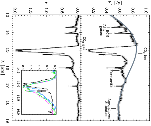
Figure 1.— Top panel: Spitzer-IRS 13$-$19 $\micron$ SH spectrum of HOPS-68, shown with statistical uncertainties (gray lines) and the adopted continuum (thick gray line). The broad absorption near 16.1 $\micron$ has been ascribed to forsterite (Mg₂SiO₄; Poteet et al., 2011), and the narrow lines at 16.0 and 17.03 $\micron$ are background-subtraction artifacts; the latter resulting from H₂ S(1) emission near the source. Bottom panel: derived optical depth spectrum of HOPS-68 (black line), centered near the strong 15.2 $\micron$ CO₂ ice $\tilde{\nu}_{2}$ bending mode. The sharp absorption feature at 14.97 $\micron$ corresponds to the blended Q-branch ro-vibrational lines of gaseous CO₂. Insert: close-up of the 14.5$-$16 $\micron$ spectrum of HOPS-68 (black line), with scaled optical depth profiles from the protostars: S140 IRS 1 (blue line; $\times$9.0), RNO 91 (green line; $\times$3.4), and IRAS 03254 (magenta line; $\times$4.5) shown for comparison.

The spectrum was extracted from the Spitzer Science Center (SSC) S18.7 pipeline basic calibrated data using the SMART software package (Higdon et al., 2004). Permanently bad and ‘rogue’ pixels were identified and corrected for by interpolation over nearby good pixels in the dispersion direction of the two-dimensional image. In order to remove sky emission from the high-resolution data we averaged the sky observations and subtracted their mean from the on-source data for HOPS-68 (catalog ). The sky subtracted two-dimensional images were averaged by nod position, and extracted using a full slit extraction. Spectra of Markarian 231 (catalog ) (LH) and $\alpha$ Lac (catalog ) (SH) were produced in the same manner, and relative spectral response functions (RSRFs) were produced by dividing a template by these spectra. Each nod of the HOPS-68 (catalog ) spectrum was then multiplied by these RSRFs to calibrate the flux density scale and the nods were averaged to obtain a final spectrum. Finally, the SH and LH spectra were scaled to the flux density of the second-order of the Long-Low spectrum (LL2; 14.2$-$20.4 $\micron$) from Poteet et al. (2011). The resultant SH spectrum is shown in the top panel of Figure 1.

II.2. Optical Depth Spectrum

We convert the CO₂ flux density to an optical depth spectrum, using: $\tau(\lambda)$ = $-\ln$($F_{\lambda}^{\rm{obs}}$/$F_{\lambda}^{\rm{cont}}$), where $F_{\lambda}^{\rm{obs}}$ and $F_{\lambda}^{\rm{cont}}$ are the observed and continuum flux densities, respectively. The continuum is constructed by fitting a third-order polynomial to the observed flux density within the wavelength ranges of 13.0$-$13.3, 14.6$-$14.7, and 18.2$-$19.5 $\micron$; the 13.5$-$14.2 $\micron$ range is avoided due to the rare gas-phase absorption of C₂H₂ (13.71 $\micron$) and HCN (14.05 $\micron$). The polynomial is then combined with a Gaussian in the wavenumber domain, with a center at $\tilde{\nu}$ = 608 cm^-1 and a Full Width at Half Maximum (FWHM) of $\Delta\tilde{\nu}$ = 73 cm^-1, to simulate the blue wing of the 18 $\micron$ silicate bending mode (Pontoppidan et al., 2008).

III. An Anomalous CO₂ Ice Band

The derived CO₂ ice optical depth spectrum of HOPS-68 (catalog ) is presented in the bottom panel of Figure 1. The profile exhibits prominent double-peaked substructure at 15.05 and 15.24 $\micron$, characteristic of pure, crystalline CO₂ ice (Hudgins et al., 1993; Ehrenfreund et al., 1997). The CO₂ bending mode profiles toward the well-studied protostars: S140 IRS 1 (catalog ), RNO 91 (catalog ), and IRAS 03254 (catalog ) are shown for comparison in the insert of Figure 1, illustrating that the HOPS-68 (catalog ) profile is fundamentally different (Pontoppidan et al., 2008; Gerakines et al., 1999). The double-peaked substructure toward these low- and high-mass protostars occurs near 15.1 and 15.23 $\micron$ and is less prominent in comparison; the dip-to-peak ratios, defined by Zasowski et al. (2009) as the local minimum to local maximum ratio of the blue peak, is 1.6$-$3.4 times less than that of HOPS-68 (catalog ). Secondly, toward these protostars a third peak or broad shoulder is often observed near 15.4 $\micron$, but is only weakly detected in the SH spectrum of HOPS-68 (catalog ). Finally, the SH spectrum of HOPS-68 (catalog ) reveals the presence of both gaseous 14.97 $\micron$ CO₂ absorption and a blue absorption component or wing shortward of 15.05 $\micron$. In comparison, gas-phase CO₂ absorption is weakly observed in the spectrum of the massive protostar S140 IRS 1 (catalog ); however, the spectrum displays no evidence for a blue wing.

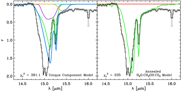
Figure 2.— Spitzer-IRS SH optical depth spectrum of HOPS-68 (black line) and best-fit CO₂ ice models. Left panel: the best-fit unique component CDE grain shape model (blue line) from Pontoppidan et al. (2008). The model includes contributions from the pure CO₂ component (T = 15 K; green line), the hydrogen-poor CO₂:CO = 112:100 mixture (T = 10 K; violet line), and the 15.4 $\micron$ shoulder component (orange line). Right panel: the best-fit annealed ice model adopted from Gerakines et al. (1999). The model consists of the annealed H₂O:CH₃OH:CO₂ = 1:0.9:1 mixture (T = 125 K; green line) and the CDE shape-corrected laboratory spectrum of the hydrogen-rich H₂O:CO₂ = 100:14 mixture (T = 10 K; red line). The fitting procedures are constrained to wavelengths shortward of 15.6 $\micron$ to avoid the blue wing of the 16.1 $\micron$ forsterite feature.

III.1. Unique Component Model

We first demonstrate that the unique component decomposition, which generally fits the CO₂ bending mode profiles in both low- and high-mass protostars, fails for HOPS-68 (catalog ). Following Pontoppidan et al. (2008), we use the following five components, corrected for shape-effects using a continuous distribution of ellipsoids (CDE; Bohren & Huffman, 1983) model: hydrogen-rich CO₂ (H₂O:CO₂ = 100:14; T = 10 K), CO-rich CO₂ (CO:CO₂ = 100:70, 100:26 or CO₂:CO = 112:100; T = 10 K), pure CO₂ (T = 15 K), and dilute CO₂ (CO:CO₂ = 100:4; T = 10 K). For the pure CO₂ component, we adopted the shape-corrected, high-resolution spectra from this work (see Appendix A). To match the resolving power of the SH module, the high-resolution spectra are convolved with a Gaussian, having a FWHM of $\Delta\lambda$ $\approx$ 0.03 $\micron$, at each wavelength element. The fifth component, often referred to in the literature as the CO₂ shoulder at 15.4 $\micron$, has been identified as an intermolecular interaction between CO₂ and CH₃OH in annealed H₂O:CH₃OH:CO₂ mixtures (Ehrenfreund et al., 1998; Dartois et al., 1999), and is empirically modeled using a superposition of two Gaussians in the wavenumber domain.

We employ a nonlinear least-squares fitting routine (MPFIT; Markwardt, 2009) to determine the best-fit scaling of each component to the observed CO₂ bending mode of HOPS-68 (catalog ):

$$\tau(\lambda)=\sum_{i=1}^{5}\alpha_{i}\tau_{i}(\lambda),$$ (1)

where $\tau_{i}(\lambda)$ is the normalized optical depth of an individual laboratory ice component and $\alpha_{i}$ is its corresponding scaling parameter. The fit is performed over the wavelength ranges of 14.75$-$14.95 and 15.0$-$15.6 $\micron$ to avoid the gas-phase CO₂ absorption at 14.97 $\micron$ and the blue wing of the 16.1 $\micron$ forsterite feature.

A comparison between the best-fit model and the observed CO₂ bending mode of HOPS-68 (catalog ) is shown in the left panel of Figure 2, and clearly indicates that the ice composition is poorly simulated ($\chi_{\nu}^{2}$ $\approx$ 391) by the unique component decomposition from Pontoppidan et al. (2008). The best-fit model results in a three-component ice mantle that is dominated by pure CO₂, with contributions from the CO-rich CO₂:CO = 112:100 mixture and the 15.4 $\micron$ shoulder component. The hydrogen-rich H₂O:CO₂ = 100:14 mixture, which generally dominates the bending mode profiles toward low- and high-mass protostars (Pontoppidan et al., 2008; Gerakines et al., 1999; Oliveira et al., 2009; Seale et al., 2011; An et al., 2011; Kim et al., 2012), is entirely absent from the model. The red wing of the observed profile is adequately matched by the pure CO₂ component, however the blue peak (15.14 $\micron$) of the pure CO₂ spectrum does not coincide with the observed peak position of 15.05 $\micron$. Moreover, we find that the CO-rich CO₂:CO = 112:100 mixture is too broad and redshifted to account for the observed blue wing of the bending mode; decreasing the CO₂ fraction of this mixture results in a narrow profile that becomes further redshifted.

III.2. Annealed H₂O:CH₃OH:CO₂ Model

We now consider the approach from Gerakines et al. (1999), who first interpreted the CO₂ bending mode profiles toward high-mass protostars using a combination of a hydrogen-rich mixture and an annealed CH₃OH-rich mixture. Similarly to Seale et al. (2011), a two-component model was assembled using the CDE shape-corrected H₂O:CO₂ = 100:14 (T = 10 K) mixture and an annealed H₂O:CH₃OH:CO₂ mixture from the large library of laboratory spectra described in White et al. (2009). However, since the blue peak of the observed bending mode is positioned near 15.05 $\micron$, we consider only the bluest ($\tilde{\nu}$ $\gtrsim$ 662 cm^-1 or $\lambda$ $\lesssim$ 15.1 $\micron$) H₂O:CH₃OH:CO₂ spectra for simplicity. The annealed mixtures are described in Table 1. For consistency with other studies (e.g., Gerakines et al., 1999; Cook et al., 2011), grain shape corrections were not applied to the absorption spectra of annealed mixtures; the segregation of CH₃OH and CO₂ in laboratory ice mixtures is thought to result in a highly inhomogeneous structure that is no longer well represented by thin films (Gerakines et al., 1999; Ehrenfreund et al., 1999).

Table 1Summary of Laboratory Absorption Spectra

Ice	Mixture	T	Resolution
Composition	Ratio	(K)	(cm-1)
Hydrogen-rich Ice (Ehrenfreund et al., 1997)
H2O:CO2	100:14	10	1
Hydrogen-poor Ices (Ehrenfreund et al., 1997)
CO:CO2	100:4	10	1
CO:CO2	100:4	30	1
CO:CO2	100:8	10	1
CO:CO2	100:8	30	1
CO:CO2	100:16	10	1
CO:CO2	100:16	30	1
CO:CO2	100:21	10	1
CO:CO2	100:21	30	1
CO:CO2	100:23	10	1
CO:CO2	100:23	30	1
CO:CO2	100:26	10	1
CO:CO2	100:26	30	1
CO:CO2	100:70	10	1
CO:N2:CO2	100:50:20	10	1
CO:N2:CO2	100:50:20	30	1
CO:O2:CO2	100:10:23	10	1
CO:O2:CO2	100:10:23	30	1
CO:O2:CO2	100:11:20	10	1
CO:O2:CO2	100:11:20	30	1
CO:O2:CO2	100:20:11	10	1
CO:O2:CO2	100:20:11	30	1
CO:O2:CO2	100:50:4	10	1
CO:O2:CO2	100:50:4	30	1
CO:O2:CO2	100:50:8	10	1
CO:O2:CO2	100:50:16	10	1
CO:O2:CO2	100:50:16	30	1
CO:O2:CO2	100:50:21	10	1
CO:O2:CO2	100:50:21	30	1
CO:O2:CO2	100:50:32	10	1
CO:O2:CO2	100:54:10	10	1
CO:O2:CO2	100:54:10	30	1
CO:O2:N2:CO2	100:50:25:32	10	1
CO:O2:N2:CO2	100:50:25:32	30	1
CO:O2:N2:CO2:H2O  . . .	25:25:10:13:1	10	1
CO:O2:N2:CO2:H2O	50:35:15:3:1	10	1
CO:O2:N2:CO2:H2O	50:35:15:3:1	30	1
CO2:CO	112:100:1	10	1
CO2:CO	112:100:1	45	1
CO2:H2O	6:1	10	1
CO2:H2O	6:1	42	1
CO2:H2O	6:1	45	1
CO2:H2O	6:1	50	1
CO2:H2O	6:1	55	1
CO2:H2O	6:1	75	1
CO2:H2O	10:1	10	1
CO2:H2O	10:1	80	1
CO2:H2O	100:1	10	1
CO2:H2O	100:1	30	1
CO2:O2	1:1	10	1
Pure CO2 Ices (This Work)
Pure CO2	$\cdots$	15	1.0.1
Pure CO2	$\cdots$	30	1.0.1
Pure CO2	$\cdots$	45	1.0.1
Pure CO2	$\cdots$	60	1.0.1
Pure CO2	$\cdots$	75	1.0.1
Annealed Ices (White et al., 2009)
H2O:CH3OH:CO2	1:0.9:1	125	1
H2O:CH3OH:CO2	1:0.9:1	130	1
H2O:CH3OH:CO2	1:1.7:1	110	1
H2O:CH3OH:CO2	1:1.7:1	115	1
H2O:CH3OH:CO2	1:1.7:1	120	1

The best-fit model is presented in the right panel of Figure 2. In contrast to past studies (e.g., Gerakines et al., 1999; Seale et al., 2011), we find that combining the CDE shape-corrected hydrogen-rich H₂O:CO₂ = 100:14 (T = 10 K) mixture with an annealed H₂O:CH₃OH:CO₂ = 1:0.9:1 (T = 125 K) mixture yields a poor goodness of fit ($\chi_{\nu}^{2}$ $\approx$ 235). In particular, we find that the hydrogen-rich mixture, which is known to consistently dominate the bending mode, is simply not utilized by the nonlinear least-squares fitting routine due to its broad redshifted profile. Instead, the fitting routine attempts to constrain the ice composition with a single annealed mixture. However, even for the bluest annealed mixtures, we find that the position of the blue peak does not coincide with the observed peak position of $\sim$15.05 $\micron$. This result demonstrates that the observed CO₂ bending mode cannot be modeled by combining a hydrogen-rich mixture with an annealed H₂O:CH₃OH:CO₂ mixture, or by a single annealed H₂O:CH₃OH:CO₂ mixture. Moreover, this is consistent with the fact that the unique profile decomposition is capable of simulating the same lines-of-sight as the annealed ice mixtures (Pontoppidan et al., 2008).

III.3. Multi-Component Homogeneous Spheres Model

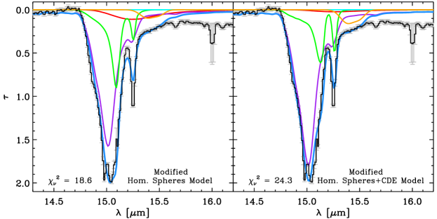
Figure 3.— Spitzer-IRS SH optical depth spectrum of HOPS-68 (black line) and best-fit CO₂ ice models (blue lines). Left panel: the best-fit multi-component homogeneous spheres model. Individual CO₂ ice components include: hydrogen-poor CO₂ CO₂:H₂O = 6:1 mixture (T = 55 K; violet line), pure CO₂ (T = 15 K; green line), hydrogen-rich H₂O:CO₂ = 100:14 mixture (T = 10 K; red line), and the 15.4 $\micron$ shoulder (orange line). Right panel: the best-fit multi-component CDE + spheres model. A line-of-sight consisting of two grain shape populations was simulated by combining the CDE shape-corrected laboratory spectra of pure CO₂ ice (T = 75 K; green line) and the hydrogen-rich H₂O:CO₂ = 100:14 mixture (T = 10 K; red line), with the homogeneous CO₂:H₂O = 6:1 spheres mixture (T = 55 K; violet line).

Having found that the traditional methods for analyzing the CO₂ ice band profile fail for HOPS-68 (catalog ), we now investigate a broader set of possibilities. In particular, we must include a component that can provide additional absorption in the blue wing of the profile. To this end, we consider additional CO₂-bearing, hydrogen-poor ice analogs from Ehrenfreund et al. (1997) and explore the effect of grain shape by using homogeneous spheres in the Rayleigh limit. The hydrogen-poor mixtures, which are summarized in Table 1, consist of two or more molecular constituents and span a laboratory temperature range of T = 10$-$80 K. Grain shape-corrected spectra for a variety of particle shape distributions are presented by Ehrenfreund et al. (1997). For relatively dilute CO₂ (e.g., H₂O:CO₂ = 100:14 and CO:CO₂ = 100:26), grain shape effects are generally weak, and only minor differences in the bending mode profile exist between the CDE and spherical grain shape corrections. Conversely, for CO₂-rich mixtures (e.g., pure CO₂ and CO₂:H₂O = 6:1), spherical grain shape corrections often result in a narrow blueshifted profile that is qualitatively consistent with the observed blue wing.

Following a similar methodology as before, a spectral decomposition of the observed bending mode was performed using the multi-component model from Pontoppidan et al. (2008). However, for this model, the choice of the hydrogen-poor CO₂ component was not restricted to the three CO-rich mixtures used by Pontoppidan et al. (2008), but instead selected from the aforementioned suite of CO₂-bearing ice analogs by Ehrenfreund et al. (1997). The laboratory temperature of the pure CO₂ component was also permitted to vary from T = 15$-$75 K. Furthermore, we assume that the line-of-sight consists exclusively of small homogeneous spheres.

Table 2Column Densities and Abundances for Best-fit CO₂ Ice Models

Grain Shape	N(CO2)	H-rich	CO-rich	Pure	Shoulder	Dilute	H-poor	Tpure	$\chi_{\nu}^{2}$
Model	(1017 cm-2)	(%)	(%)	(%)	(%)	(%)	(%)	(K)
Multi-component Models
CDE	19.83 $\pm$ 0.49	$\cdots$	27 $\pm$ 3	65 $\pm$ 3	8 $\pm$ 12	$\cdots$	$\cdots$	15	391.1
Spheres	24.66 $\pm$ 0.59	10 $\pm$ 13	$\cdots$	22 $\pm$ 3	3 $\pm$ 11	$\cdots$	65 $\pm$ 3	15	118.6
CDE$+$Spheres $\,.\,.\,$	24.53 $\pm$ 0.59	12 $\pm$ 52	$\cdots$	18 $\pm$ 3	6 $\pm$ 18	$\cdots$	74 $\pm$ 3	75	124.3
Median Abundance Toward Low-mass Protostars (Pontoppidan et al., 2008)
CDE	8.46${}^{16.20}_{\phantom{1}4.34}$	70${}^{74}_{65}$	20${}^{27}_{15}$	6${}^{12}_{\phantom{1}1}$	3${}^{5}_{2}$	$<$0.1${}^{1}_{0}$	$\cdots$	15	$\cdots$

Note. — Uncertainties are based on statistical errors in the Spitzer-SH spectrum and systematic errors in the continuum determination. Grain shape models from this work include: irregular grains (CDE), pure homogeneous spheres (spheres), and two separate grain shape populations (CDE+Spheres). For the CDE and spheres models, all CO₂ components consist of irregularly-shaped particles and homogeneous spheres, respectively. For the CDE+spheres model, all components are representative of irregularly-shaped particles, except for the hydrogen-poor CO₂ component which is representative of homogeneous spheres.

The best-fit homogeneous spheres model is presented in the left panel of Figure 3. A four-component model, consisting largely of pure CO₂ (T = 15 K) and the hydrogen-poor CO₂:H₂O = 6:1 (T = 55 K) mixture, was found to provide the best fit ($\chi_{\nu}^{2}$ $\approx$ 19) to the observed bending mode. As qualitatively expected, we find that the observed blue wing is adequately simulated by spherical grain shape-corrected laboratory spectra of CO₂-rich mixtures. Furthermore, the observed red wing is well matched by a combination of pure CO₂, the hydrogen-rich H₂O:CO₂ = 100:14 (T = 10 K) mixture, and the 15.4 $\micron$ shoulder component. However, due to the relatively low amplitude of the pure CO₂ red peak, the optical depth of the 15.24 $\micron$ peak is slightly under-predicted by the best-fit model. Nonetheless, we conclude that an exclusive homogenous spheres model, consisting predominately of the hydrogen-poor CO₂:H₂O = 6:1 (T = 55 K) mixture, yields an overall excellent fit to the observed CO₂ bending mode profile.

III.4. Homogeneous Spheres + CDE Model

The grain shapes of CO and CO₂ ice mantles in the circumstellar envelopes of protostars have been constrained using multiple ice bands of the same species (Boogert et al., 2002; Pontoppidan et al., 2003; Gerakines et al., 1999). A simultaneous decomposition of these bands indicates that their observed profiles are consistent with those of small irregularly-shaped ice mantles, simulated by CDE grain shape models. For this reason, invoking a model consisting exclusively of homogeneous spheres may seem unjustified. However, we have demonstrated that utilizing a CDE grain shape model to simulate the CO₂ bending mode of HOPS-68 (catalog ) is largely unsatisfactory. Even when the choice of the hydrogen-poor component is not constrained to the CO-rich CO:CO₂ mixtures used by Pontoppidan et al. (2008), we find that the goodness of fit is generally poor ($\chi_{\nu}^{2}$ $\approx$ 90$-$680). Although our analysis is restricted to laboratory experiments for which grain shape corrections have been applied, this result implies that the observed blue wing is inconsistent with all available CDE shape-corrected hydrogen-poor ice analogs. In contrast, we have shown that small homogeneous spheres of the hydrogen-poor CO₂:H₂O = 6:1 (T = 55 K) ice mixture can adequately fit the blue wing of the observed bending mode.

To further examine the robustness of this result, we next consider a modeled line-of-sight that is populated by both spherical and irregularly-shaped grains. Following a similar approach as in Section III.3, a CO₂ ice model was constructed by combining the previously utilized CDE shape-corrected laboratory spectra (hydrogen-rich CO₂, pure CO₂, and dilute CO₂), a spherical grain shape-corrected hydrogen-poor laboratory spectrum, and the empirical 15.4 $\micron$ CO₂ shoulder component. The best-fit model is shown in the right panel of Figure 3. Indeed, we find that a four-component model, composed largely of the same homogeneous CO₂:H₂O = 6:1 (T = 55 K) spheres mixture from Section III.3, is required for a satisfactory fit ($\chi_{v}^{2}$ $\approx$ 24). The red wing of the observed bending mode is well matched by the combination of the CDE shape-corrected spectra of pure CO₂ (T = 75 K) and the hydrogen-rich H₂O:CO₂ = 100:14 (T = 10 K) mixture, with the 15.4 $\micron$ shoulder component. In comparison to the model results from Section III.3, we conclude that a modeled line-of-sight composed of two separate grain shape populations (spherical and irregularly-shaped particles) provides an equally good fit. This result demonstrates that the CO₂ bending mode profile toward HOPS-68 (catalog ) is largely governed by the grain shape and chemical composition of the hydrogen-poor CO₂ component.

III.5. CO₂ Ice Column Density

The column density along the line-of-sight for each best-fit CO₂ component was estimated from Equation A2, adopting the pure CO₂ bending mode band strength of A = 1.1 $\times$ 10^-17 cm molecule^-1 from Gerakines et al. (1995). The optical depth spectra were integrated over the wavenumber range of 680.3$-$613.5 cm^-1 ($\lambda$ = 14.7$-$16.3 $\micron$) to include the long wavelength wing of the observed profile.

To estimate the systematic contribution from the baseline subtraction, we first computed the standard error, $\sigma$, between the best-fit continuum and the SH spectrum. The best-fit continuum was then offset by $\pm$1 $\sigma$ to produce new optical depth spectra and column density estimates. To quantify the errors due to the baseline uncertainty, we then calculated the mean absolute difference between the best-fit column densities and the column densities obtained by offsetting the best-fit continuum. These errors were then added in quadrature with the best-fit errors, which are returned by the least-squares minimization technique, to generate the final CO₂ ice column density uncertainties.

The column densities and relative abundances for the best-fit CO₂ ice models are tabulated in Table 2. The modified spectral decomposition analysis gives us the following three observables: 1) Among the available laboratory ice analogs, homogeneous spheres of the hydrogen-poor CO₂:H₂O = 6:1 (T = 55 K) mixture are required to match the blue wing of the observed CO₂ bending mode. This component constitutes 65$-$74% of the total CO₂ ice column density along the line-of-sight. 2) The red wing of the observed profile can be modeled by combining pure CO₂ ice and the 15.4 $\micron$ CO₂ shoulder component. The pure CO₂ component constitutes 18$-$22% of the total CO₂ ice column density, while only a minor (3$-$6%) contribution is attributed to the 15.4 $\micron$ CO₂ shoulder component. 3) Only 2$-$10% of the total CO₂ ice column density is composed of the hydrogen-rich component, while no evidence for the CO-rich component is found within the observed CO₂ bending mode. These fundamental differences of HOPS-68 (catalog ), as compared to the ice structure toward typical low-mass protostars, are illustrated in Table 2.

To derive the CO₂ ice abundance, the H₂O ice column density toward HOPS-68 (catalog ) was estimated from the 12 $\micron$ libration mode of the amorphous silicate-subtracted optical depth spectrum from Poteet et al. (2011). Adopting an intrinsic band strength of A = 2.9 $\times$ 10^-17 cm molecule^-1 for crystalline H₂O ice (T = 140 K; Mastrapa et al., 2009), we calculate a H₂O ice column density of N(H₂O) = 88.2 $\pm$ 0.7 $\times$ 10¹⁷ cm^-2. For the best-fit models from Sections III.3 and III.4, we calculate an average CO₂ to H₂O ice column density ratio of N(CO₂)/N(H₂O) = 0.28 $\pm$ 0.03. This is consistent with abundances measured toward low-mass protostars (N(CO₂)/N(H₂O) = 0.32 $\pm$ 0.02; Pontoppidan et al., 2008), but is significantly greater than those observed for high-mass protostars (N(CO₂)/N(H₂O) = 0.17 $\pm$ 0.03; Gerakines et al., 1999).

IV. Discussion and Conclusions

IV.1. The Rarity of Highly Processed Ice

The Spitzer-IRS SH spectrum toward the low-mass protostar HOPS-68 (catalog ) reveals a rare 15.2 $\micron$ CO₂ bending mode profile, exhibiting a prominent double-peaked substructure (near 15.05 and 15.24 $\micron$) and a strong blue absorption wing. Our analysis demonstrates that the observed bending mode cannot be modeled using the unique component models from Pontoppidan et al. (2008) or by combining a hydrogen-rich mixture with an annealed H₂O:CH₃OH:CO₂ mixture (Gerakines et al., 1999). However, when the Pontoppidan et al. (2008) models are modified to include spherical grains and a broader selection of hydrogen-poor ice mixtures, an overall excellent fit to the observed CO₂ bending mode is obtained.

Our results indicate that most (87$-$92%) of the CO₂ along the line-of-sight is present in ices where CO₂ is the dominant constituent. In contrast, the majority of the CO₂ ice observed toward most low- and high-mass protostars is found in environments dominated by H₂O and CO. For example, toward low-mass protostars, Pontoppidan et al. (2008) showed that generally $\sim$70% of the total CO₂ ice column density is composed of the hydrogen-rich component, while $\sim$20% is attributed to the CO-rich component. Furthermore, the median abundance of pure CO₂ ice to the total CO₂ ice column density is found to be $\sim$6%.

The nearly complete lack of unprocessed ice mantles along the line-of-sight toward HOPS-68 (catalog ) is unexpected. For example, toward the prominent low-mass sources IRAS 03254 (catalog ) and RNO 91 (catalog ), comparable fractions of pure CO₂ (17$-$23%) are reported by Pontoppidan et al. (2008). However, a substantial fraction (70$-$75%) of their total CO₂ ice column density is attributed to unprocessed ice mixtures (CO:CO₂ and H₂O:CO₂), which lie outside the distillation and segregation radii (Öberg et al., 2011). In this context, the ice mantles toward HOPS-68 (catalog ) are uniquely different from those observed toward other protostars, indicating that the observed icy grains have undergone a higher degree of thermal processing.

IV.2. The Origin of Processed Ice Toward HOPS-68

Nearly 100 CO₂ ice spectra have been described in the literature, and the observed profile toward HOPS-68 (catalog ) is unique among them. It is therefore unlikely to find more than a few percent of HOPS-68 (catalog ) ice analogs in a larger sample of protostars. Is this rarity due to HOPS-68 (catalog ) being fundamentally different than other protostars, or does the observed line-of-sight reveal processed ices that are present in other protostars, but which are typically obscured by their cold outer envelope?

IV.2.1 The Lack of Unprocessed Ice

A peculiar spectral property of HOPS-68 (catalog ) is the combination of a relatively flat 8$-$70 $\micron$ SED and strong silicate absorption at 9.7 $\micron$ (Poteet et al., 2011, Figure 3). To reproduce these observed characteristics, Poteet et al. (2011) employed a radiative transfer model based on the collapse of an isothermal sheet initially in hydrostatic equilibrium (Hartmann et al., 1994, 1996). They conclude that HOPS-68 (catalog ) possesses a highly flattened ($\eta$ = 2.0) protostellar envelope, as described by the degree of asphericity ($\eta$ = $R_{\rm{max}}/H$, where R_max is the outer envelope radius and H is the scale height of the initial sheet). In comparison, Furlan et al. (2008) found that most Taurus protostars do not require an initially flattened density distribution, but instead can be modeled by the collapse of an initially spherically symmetric cloud core (Terebey et al., 1984). Unlike spherical envelopes, an implication of the highly flattened structure is that cold material in the outer envelope is not expected to be present along the observed line-of-sight. Indeed, we estimate that $\lesssim$15% of the gas has temperatures below T = 30 K. Thus, the absence of the volatile CO-rich CO₂ component and the low abundance of the hydrogen-poor CO₂ component may be explained by the lack of cold, unprocessed dust along the line-of-sight. This result suggests that highly processed ices may be present in the inner regions of other protostellar envelopes, but are likely obscured or diluted by the large, cold envelopes of unprocessed material typically surrounding them.

Furthermore, to simultaneously simulate the strong silicate absorption, the Poteet et al. (2011) model requires infalling material to be deposited within 0.5 AU of the central protostar, as set by the centrifugal radius ($R_{c}$). In contrast, $R_{c}$ values from 10 to 300 AU, with a median of 60 AU, were found for Taurus protostars (Furlan et al., 2008). For a centrifugal radius of $R_{c}$ = 0.5 AU, we estimate that more than 50% of the infalling material along the line-of-sight is concentrated within 10 AU of the central protostar, where the potential for thermal processing of icy grains by radiation and outflow-induced shocks is the strongest.

Resolved images of protostellar envelopes show a wide range of envelope morphologies, from highly flattened to relative spheroidal structures, as well as a great deal of complexity (Tobin et al., 2010, 2011, 2012). The diversity of envelope morphologies may be due to formation of protostars in turbulent and often filamentary molecular clouds (e.g., André et al., 2010; Molinari et al., 2010). Although the envelope of HOPS-68 (catalog ) has not yet been resolved, SED modeling requires a highly flattened envelope which may be uncommon within the diversity of envelope morphologies typically found in molecular clouds. This flattened envelope, when observed from an intermediate inclination, results in a line-of-sight that is less obscured by unprocessed material in the cold, outer envelope.

IV.2.2 The Formation of Spherical CO₂-rich Mantles

Although a flattened envelope structure may explain the absence of cold primordial ices seen toward other protostars, it does not directly explain why a large fraction of the CO₂ ice seen toward HOPS-68 (catalog ) is sequestered as spherical, CO₂-rich mantles, while typical interstellar ices show evidence of irregularly-shaped, hydrogen-rich mantles. That is, in the absence of unprocessed ices along the line-of-sight, the observed CO₂ ice profile should be consistent with irregularly-shaped CO₂-rich ice mantles. Irregularly-shaped ice mantles are generally understood to be the product of a slow aggregation of icy grain monomers in dense molecular clouds prior to protostellar collapse (Ossenkopf, 1993; Ormel et al., 2009). In the case of HOPS-68 (catalog ), we propose that the spherical ice mantles may have formed as the volatiles rapidly freeze out in dense gas, following an energetic, but transient event that sublimated any primordial icy grain population within its inner envelope region.

Radiative processing by episodic accretion events have recently been proposed by Kim et al. (2012) to be a viable mechanism for producing pure CO₂ ice, through the distillation process, toward low-luminosity protostars (L $\lesssim$ 1 L_☉). Using the unique component decomposition from Pontoppidan et al. (2008), Kim et al. (2012) report a median pure CO₂ ice abundance of 15% toward six protostars; this value is six times less than the processed ice abundance found toward HOPS-68 (catalog ). The detection of pure CO₂ ice toward low-luminosity protostars indicates that a transient phase of higher luminosity must have existed some time in their past (Kim et al., 2012). For the case of HOPS-68 (catalog ), we propose that heating beyond the sublimation temperature of H₂O ice (T $\approx$ 110 K; Fraser et al., 2001) will evaporate ice mantles close to the central protostar during the high-luminosity phase, resulting in the separation of icy grain conglomerates. As the protostar later returns to its quiescent, low-luminosity phase, gas temperatures in the envelope decrease and H₂O and CO₂ rapidly ($t$ $<$ 10³ yr) condense onto grain surfaces in the order of their condensation temperature (Ossenkopf, 1993), provided that the gas is sufficiently dense ($n_{\rm{H_{2}}}$ $>$ $10^{4}$ cm^-3). This mechanism naturally allows for the formation of nearly pure CO₂ ice mantles sequestered on spherical grains. However, this scenario requires that the accretion outburst must have occurred recently to avoid the reproduction of irregular grains by renewed grain aggregation.

Evidence for transient heating is often presumed from the variable nature of the accretion luminosity. Photometric monitoring of HOPS-68 (catalog ), with the Herschel Space Observatory, reveal a $\sim$21% variation in the 70 $\micron$ flux over a two week period; this variability is most likely driven by variations in the mass accretion rate onto the central protostar (Billot et al., 2012). While larger increases in luminosity, over longer timescales, are certainly needed to heat dust grains to the sublimation temperature of H₂O ice, the observed variability indicates a rapidly changing accretion rate for HOPS-68 (catalog ), and hence, supports the possibility of a recent ($t$ $\ll$ $10^{6}$ yr) accretion outburst that raised the luminosity significantly above the current observed value.

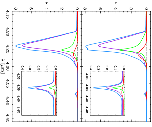
Figure 4.— Model predictions for the ($\tilde{\nu}_{3}$) ¹²CO₂ and ($\tilde{\nu}_{3}$) ¹³CO₂ stretching modes at 4.27 and 4.38 $\micron$, respectively. The predicted CO₂ profiles (blue lines) are constructed from the best-fit multi-component homogeneous spheres model (Section III.3; top panel) and the multi-component CDE + homogeneous spheres model (Section III.4; bottom panel). The individual ice components include: hydrogen-rich CO₂ (H₂O:CO₂ = 100:14 at T = 10 K; red lines), hydrogen-poor CO₂ (CO₂:H₂O = 6:1 at T = 55 K; violet lines), and pure CO₂ (T = 15 and 75 K; green lines).

In order to quantify the luminosity rise needed to produced the proposed sublimation of icy grains, we increase the total luminosity of the Poteet et al. (2011) SED model by a factor of 10, 50, and 100. Adopting a CO₂ ice desorption temperature of T = 45 K, from an amorphous H₂O ice surface (Noble et al., 2012), we assume that CO₂ ice is present in the envelope of HOPS-68 (catalog ) at distances greater than r $\approx$ 90 AU. These incremental steps in luminosity result in increased dust temperatures of T = 70, 97, and 113 K at r $\approx$ 90 AU, respectively. Thus, for HOPS-68 (catalog ), we propose that a factor of 100 increase in luminosity ($\sim$100 L_☉) is required to thermally desorb CO₂ and H₂O ices from the surface of dust grains. Although the required luminosity is higher than the typical luminosities of protostars in Orion ($\sim$1 L_☉; Kryukova et al., 2012), luminosities in excess of 100 L_☉ are observed toward young, low-mass stars undergoing FU Orions-like outbursts (Reipurth & Aspin, 2010). Kryukova et al. (2012) finds five Orion protostars with luminosities exceeding 100 L_☉, including two candidate FU Orionis-like objects. Furthermore, models developed to explain the typical low luminosities of protostars require that most low-mass protostars undergo FU Orionis-like outbursts in order to accrete the required amount of mass during the protostellar lifetime (Dunham & Vorobyov, 2012).

Alternatively, mechanical processing by shocks, associated with the observed outflow (Williams et al., 2003), will also sublimate ice mantles in the outflow working surface along the cavity wall. In dense shocks, dust grain temperatures are raised by collisional heating with hot gas particles and by absorption of photons as the compressed gas cools, resulting in thermal desorption and sputtering of interstellar ices. In particular, for a nondissociative shock with a velocity of $v_{s}$ = 10 km s^-1, dust grains are expected to be heated to temperatures on the order of 10² K (Neufeld & Hollenbach, 1994), which is more than sufficient to allow for a condensation sequence to occur behind the shock. Therefore, similar to the accretion outburst scenario, we propose that nearly pure CO₂ ice mantles are formed in post-shocked gas, again in a condensation sequence, which the line-of-sight must be dominated by shock-processed material near the cavity wall. For other orientations, the line-of-sight will be dominated by irregularly-shaped icy grain mantles. Toward HOPS-68 (catalog ), evidence for the presence of shock-processing may be inferred from the detection of [S I], [Fe II], and [Si II] forbidden emission at 25.25, 25.98, and 34.82 $\micron$, respectively (D. M. Watson et al. 2013, in preparation), as well as gaseous absorption from C₂H₂, HCN, and CO₂ at 13.71, 14.05, and 14.97 $\micron$, respectively.

We note that the formation of interstellar ices in a post-shocked gas was originally proposed by Bergin et al. (1998, 1999). However, in their scenario, CO₂ ice is formed by virtue of gas-phase reactions (CO + OH $\rightarrow$ CO₂ + H) and subsequent freeze-out. The formation process is largely governed by the photodissociation rate of H₂O molecules by cosmic-ray induced photons, and is expected to occur over a timescale of t $\approx$ 10⁵ yr at the assumed density of $n_{\rm{H_{2}}}$ = $10^{5}$ cm^-3; however, the timescale may be shortened with higher gas densities or larger cosmic-ray ionization rates. Nonetheless, this long timescale for CO₂ ice mantle formation would allow for the re-development of irregularly-shaped grains, through the aggregation of small regular particles. In contrast, the detection of spherical icy grains implies that ice mantle formation would have occurred more recently, over much shorter timescales (t $\sim$ $\mathcal{O}$(10²) yr) and at higher densities ($n_{\rm{H_{2}}}$ $\approx$ $10^{7}$ cm^-3 at $r$ = 100 AU), by evaporation and re-condensation processes alone.

In summary, we propose that the observed 15.2 $\micron$ CO₂ ice profile may result from the combination of two circumstances. First, the nearly complete absence of unprocessed ices along the line-of-sight is due to the highly flattened envelope of HOPS-68 (catalog ), which lacks cold absorbing material in its outer envelope, and possesses a large fraction of material within its inner (10 AU) envelope region. Second, an energetic event led to the evaporation of inner envelope ices, followed by cooling and re-condensation, explaining the sequestration of CO₂ in a hydrogen-poor mixture and the spherical shape of the icy grains. Regardless of which energetic process is responsible for producing the spherical mantles, we note that both proposed mechanisms require fortuitous timing and orientations, and hence are consistent with the observed rarity of spherical icy grains toward protostars.

The notion of ices forming in a cooling gas, following an energetic event, makes several predictions. Water ice condensed at high temperatures will arrange itself into a crystalline matrix, predicting that the H₂O ice seen toward HOPS-68 (catalog ) should be predominantly crystalline. Evidence for the presence of crystalline H₂O ice was predicted, by Poteet et al. (2011), from the 12 $\micron$ libration mode. This prediction can be further tested by observing the profile of the 3.08 $\micron$ H₂O stretching mode. Carbon monoxide ice, observed at 4.67 $\micron$, should either be absent if the temperature of the absorbing material is still above 20 K, or should show evidence of spherical grain shapes, in sharp contrast to that observed toward typical protostars (Pontoppidan et al., 2003). Finally, the ¹²CO₂ and ¹³CO₂ stretching modes at 4.27 and 4.38 $\micron$, respectively, should be consistent with spherical grains and a nearly pure CO₂ mixture. Using the best-fit models from Sections III.3 and III.4, predictions for the ¹²CO₂ and ¹³CO₂ stretching modes are presented in Figure 4. While HOPS-68 (catalog ) is too faint at 3$-$5 $\micron$ for current spectrometers, these tests will likely be within reach of the James Webb Space Telescope.

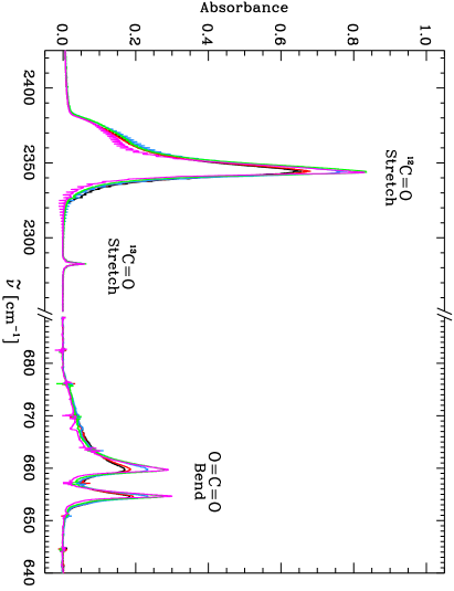
Figure 5.— The background- and baseline-corrected absorption spectra of pure CO₂ ice. The ($\tilde{\nu}_{3}$) ¹²CO₂ and ($\tilde{\nu}_{3}$) ¹³CO₂ stretching (2343 and 2283 cm^-1, respectively) and ($\tilde{\nu}_{2}$) ¹²CO₂ bending (660 and 655 cm^-1) modes are shown at laboratory temperatures of $T$ = 15 (black line), 30 (red line), 45 (blue line), 60 (green line), and 75 K (magenta line). Gas-phase CO₂ at 668 cm^-1 is a background-subtraction artifact, arising from either under- or over-subtraction of background CO₂ gas.

Appendix A Pure CO₂ Ice Laboratory Spectra

The infrared absorption bands of CO₂ have been extensively studied in the laboratory by Hudgins et al. (1993), Ehrenfreund et al. (1997), and Baratta & Palumbo (1998). Collectively, these studies present absorption spectra and optical constants for pure CO₂ at laboratory temperatures of T = 10, 12, 30, 50, 70, and 80 K. These experiments are conducted under high-vacuum conditions at a spectral resolution of 1$-$2 cm^-1, too low to fully resolve the narrow structure of the Davydov split. More recently, CO₂ experiments with a spectral resolution of 0.5 cm^-1 have been conducted at laboratory temperatures of T = 15$-$90 K (van Broekhuizen et al., 2006), but at relatively low signal-to-noise.

In this paper, we deploy new high-quality infrared absorption spectra and optical constants from a temperature-series laboratory study of pure, crystalline CO₂ ice. The experiments were conducted at an improved spectral resolution of 0.1 cm^-1 and at higher signal-to-noise with respect to previous laboratory studies.

A.1. Experimental Procedure

Following the procedures of Gerakines et al. (1995) and Bouwman et al. (2007), the experiments are performed in a high vacuum (HV) chamber with a base pressure of P $\approx$ 5$\times$10^-7 mbar at room temperature. The chamber houses a CsI (Caesium Iodide) substrate that is cooled down to 15 K by a closed cycle helium cryostat (ADP DE-202). The substrate temperature is controlled with a resistive heater element and a silicon diode sensor using an external control unit (LakeShore 330).

A sample of CO₂ (Praxair, 99.998 $\%$ purity) is introduced into the system from a gas bulb at 10.0 mbar prepared in a separate vacuum manifold (base pressure of P $\approx$ 10^-5 mbar). Pure CO₂ ices are grown onto the substrate at 15 K via effusive dosing along the surface normal at a deposition rate of $\sim$10¹⁵ molecules cm^-2 s^-1. The ices are heated to temperatures of T = 15, 30, 45, 60, and 75 K at a rate of 2 K min^-1 and allowed to relax at each temperature for five minutes before recording the absorption spectra. A Fourier Transform InfraRed (FTIR) spectrometer (Varian 670-IR) is used to record the ice spectra in transmission mode over the wavenumber range of $\tilde{\nu}$ = 4000$-$400 cm^-1 ($\lambda$ = 2.5$-$25 $\micron$) with a spectral resolution of 0.1 cm^-1, averaging a total of 256 scans to increase the signal-to-noise ratio. Background spectra are acquired at 15 K prior to deposition and subtracted from the recorded ice spectra.

A.2. Experimental Results

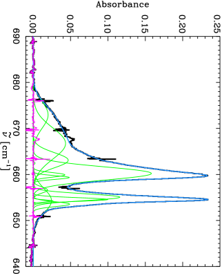
Figure 6.— The $\tilde{\nu}_{2}$ bending mode spectrum of pure CO₂ ice (black line) compared to its corresponding “smoothed” spectrum (blue line) at T = 45 K. A least-squares fit is performed using a superposition of Gaussians (green lines) to eliminate noise and gas-phase CO₂ absorption at 668 cm^-1. The resultant fit residuals (magenta line) are shown for comparison.

To facilitate a comparison with astronomical spectra, a baseline correction is applied to all laboratory absorption spectra by fitting a third-order polynomial over the wavenumber regions of 4000$-$3800, 2900$-$2700, 2270$-$2250, 950$-$700, and 645$-$640 cm^-1. The background- and baseline-corrected absorption spectra for pure CO₂ ice are shown in Figure 5 for the ($\tilde{\nu}_{3}$) ¹²CO and ($\tilde{\nu}_{3}$) ¹³CO stretching and ($\tilde{\nu}_{2}$) CO₂ bending vibrational modes.

The spectra do not suffer from any significant contamination by background gases of H₂O within the vacuum system. However, weak traces of gaseous CO₂, near 668 cm^-1 ($\lambda$ = 14.97 $\micron$), are present in some absorption spectra, and are the result from either an under- or over-subtraction of background CO₂ gas. To reduce the noise and eliminate the gas-phase CO₂ absorption, a nonlinear least-squares minimization is simultaneously performed to the $\tilde{\nu}_{3}$ ¹²CO, $\tilde{\nu}_{3}$ ¹³CO, and $\tilde{\nu}_{2}$ CO₂ vibrational modes using a superposition of Gaussians. Figure 6 illustrates the ‘smoothing’ technique for the $\tilde{\nu}_{2}$ bending mode spectrum at $T$ = 45 K. The measured peak positions ($\tilde{\nu}$) and widths (FWHM; $\Delta\tilde{\nu}$) of the $\tilde{\nu}_{2}$ bending mode are listed in Table 3. The position of the absorption peaks near 654.5 and 659.7 cm^-1 are temperature-independent and remain constant to within 0.1 cm^-1, while their FWHMs decrease by a factor of two with increasing temperature from T = 15 to 75 K. These results are in agreement with the 0.5 cm^-1 resolution study by van Broekhuizen et al. (2006).

A.3. Optical Constants

The complex index of refraction (n + ik) is determined using a Kramers-Kronig analysis, following similar methods previously described in Hudgins et al. (1993) and Mastrapa et al. (2009).

Briefly, the imaginary part of the complex refractive index, k, is calculated from the Beer-Lambert law:

$$\alpha(\tilde{\nu})\equiv 4\pi k\tilde{\nu}=\frac{1}{d}\ln\negthinspace\left(10\right)A_{\tilde{\nu}},$$ (A1)

where $\alpha$ is the Lambert absorption coefficient, d is the thickness of the ice, and $A_{\tilde{\nu}}$ is the absorbance of the ice at wavenumber $\tilde{\nu}$. The thickness of the ice samples were estimated using the known absorption band strength of pure CO₂ ice. In this technique, the column density, N (in molecules cm^-2), of the sample was determined using

$$N=\frac{\int\tau_{\tilde{\nu}}\,d\tilde{\nu}}{A},$$ (A2)

where $\tau_{\tilde{\nu}}$ = $\ln$(10)$A_{\tilde{\nu}}$ is the optical depth and A is the intrinsic band strength of the $\tilde{\nu}_{2}$ bending mode as determined from previous laboratory studies (A = 1.1$\times$10^-17 cm molecule^-1; Gerakines et al., 1995). The ice thickness is then inferred from the derived column density assuming a monolayer (ML) surface coverage of $\sim$10¹⁵ molecules cm^-2. The final ice thickness is tabulated in Table 3 and ranges in value from 355$-$410 ML. Assuming a monolayer thickness of 5.54 Å, the lattice constant for solid CO₂ (Keesom & Köhler, 1934), these values correspond to a physical thickness of $\sim$0.20$-$0.23 $\micron$.

Table 3Band Positions and FWHMs of the $\tilde{\nu}_{2}$ CO₂ Bending Mode

T	$\tilde{\nu}$	FWHM, $\Delta\tilde{\nu}$	Ice Thickness, d
(K)	(cm-1)	(cm-1)	(ML)	($\micron$)
Laboratory Spectrum
15	654.5/659.7	2.1/5.3	366	0.203
30	654.5/659.8	2.0/4.3	367	0.203
45	654.5/659.7	1.8/3.6	410	0.227
60	654.6/659.7	1.5/2.9	405	0.224
75	654.7/659.7	1.1/2.3	355	0.197
CDE Model
15	654.9/660.6	2.1/7.7	$\cdots$	$\cdots$
30	655.0/660.7	2.1/6.6	$\cdots$	$\cdots$
45	655.0/660.7	1.9/5.3	$\cdots$	$\cdots$
60	655.1/661.0	1.7/4.6	$\cdots$	$\cdots$
75	655.3/661.0	1.6/4.3	$\cdots$	$\cdots$
Homogeneous Spheres Model
15	655.6/662.6	1.4/3.6	$\cdots$	$\cdots$
30	655.6/662.5	1.3/2.4	$\cdots$	$\cdots$
45	655.6/662.4	1.1/0.9	$\cdots$	$\cdots$
60	655.6/662.3	0.9/0.5	$\cdots$	$\cdots$
75	655.8/662.4	0.6/0.3	$\cdots$	$\cdots$
Ice-coated Spheres Model
15	655.0/660.4/666.4	2.0/13.7	$\cdots$	$\cdots$
30	655.0/660.4/665.8	1.9/12.8	$\cdots$	$\cdots$
45	655.0/660.4/664.8	1.7/19.6	$\cdots$	$\cdots$
60	655.1/660.5/664.4	1.4/16.3	$\cdots$	$\cdots$
75	655.2/660.6/664.4	0.7/14.8	$\cdots$	$\cdots$

Note. — The band position and FWHM are listed for the multiple peaks within the CO₂ bending mode.

Given the absorption coefficient, the real part of the complex refractive index, n, is then calculated from the Kramers-Kronig dispersion relationship:

$$n(\tilde{\nu})=n_{0}+\frac{1}{2\pi^{2}}\thinspace\mathscr{P}\negthinspace\int_{400}^{4000}\frac{\alpha(\tilde{\nu}^{\prime})}{\tilde{\nu}^{\prime 2}-\tilde{\nu}^{2}}\,d\tilde{\nu}^{\prime},$$ (A3)

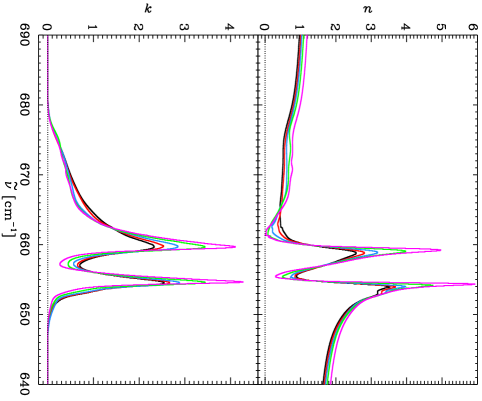
Figure 7.— The optical constants (n and k) for the $\tilde{\nu}_{2}$ bending mode of pure CO₂ ice at laboratory temperatures of T = 15 (black line), 30 (red line), 45 (blue line), 60 (green line), and 75 K (magenta line).

where $\mathscr{P}$ denotes the Cauchy principal value of the integral and $n_{0}$ is the refractive index for the high-wavenumber end of the infrared spectrum ($\tilde{\nu}$ $>$ 4000 cm^-1). Because the visible ($\lambda=0.633$ $\micron$) refractive index of pure CO₂ ice is temperature-dependent, we adopt values of $n_{0}$ $\approx$ 1.23, 1.26, 1.29, and 1.34 for the laboratory temperatures of T = 15, 30, 45, and 60 K, respectively (Satorre et al., 2008). For the absorption spectrum at T = 75 K, we use a value of $n_{0}$ $\approx$ 1.44 from Seiber et al. (1971) to ensure that n is positive for all wavenumbers. Optical constants for the $\tilde{\nu}_{2}$ bending mode of pure CO₂ are presented in Figure 7.

While our study is not intended to address the differences between the CO₂ optical constants derived in this work and those found among the literature, we do note, however, that any discrepancies are most likely due to differences in ice sample thickness and the $n_{0}$ refractive index for the high-wavenumber region ($\tilde{\nu}$ $>$ 4000 cm^-1). For a thorough discussion on the discrepancies between CO₂ optical constants derived from different studies, we refer the reader to Ehrenfreund et al. (1997).

A.4. Grain Size and Shape Corrections

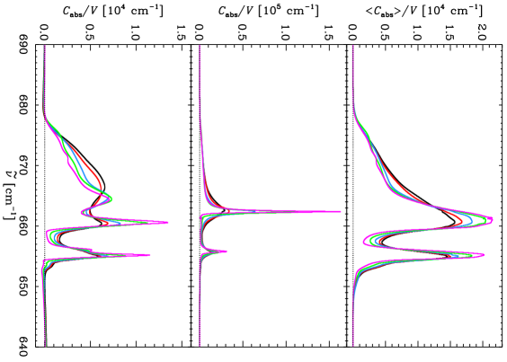
Figure 8.— The absorption cross section per unit volume for the $\tilde{\nu}_{2}$ bending mode of pure CO₂ ice. Grain shape models in the Rayleigh limit are shown for a continuous distribution of ellipsoids (CDE; top panel), homogeneous spheres (middle panel), and ice-coated silicate spheres (bottom panel) at laboratory temperatures of T = 15 (black line), 30 (red line), 45 (blue line), 60 (green line), and 75 K (magenta line).

The profiles of strong infrared resonance features, including those of ices, depend significantly on the shape and size of the absorbing and scattering particles (Tielens, 1991; Dartois, 2006). For pure CO₂ ice, grain size and shape corrections must be applied to the laboratory absorption spectra of thin films to allow for an accurate comparison to astronomical spectra. While irregularly-shaped grain models have been largely successful at simulating astronomical spectra of CO and CO₂ ices (Pontoppidan et al., 2003; Gerakines et al., 1999), we also consider here the shape effects of spherical grain models.

Using the derived optical constants of pure CO₂, standard formulae from Bohren & Huffman (1983) were applied in the Rayleigh limit to calculate the absorption cross section per unit volume, C_abs/V, for a continuous distribution of ellipsoids (CDE; all shapes are equally probable), homogeneous spheres, and ice-coated amorphous silicate spheres. For the ice-coated spheres model, we adopt amorphous silicate optical constants from Draine & Lee (1984) and assume that half of the total particle volume is occupied by the core. Note, however, for thick ice mantles or silicate cores that occupy $\lesssim$ 10% of the total particle volume, the ice-coated spheres profile approximates that of pure homogeneous spheres.

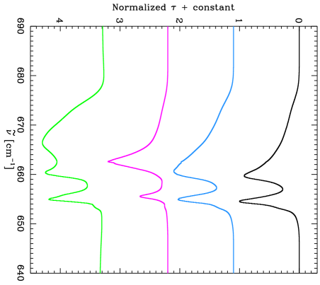
Figure 9.— The normalized optical depth profiles for the $\tilde{\nu}_{2}$ bending mode of pure CO₂ ice. The uncorrected laboratory spectrum at T = 15 K (black line) is compared to three standard grain shape models in the Rayleigh limit: a continuous distribution of ellipsoids (CDE; blue line), homogeneous spheres (magenta line), and ice-coated amorphous silicate spheres (green line).

The absorption cross sections for the bending mode of CO₂ are presented in Figure 8 for the different grain shape models. The CDE model produces a broad double-peaked absorption profile that remains mostly constant with increasing temperature from T = 15 to 75 K; the peak positions exhibit a blueshift of 0.4 cm^-1 at T = 75 K. Conversely, a narrow double-peaked structure is generated by the homogenous spheres model, whose FWHMs become narrower with increasing temperature; the FWHM of the 662.5 cm^-1 peak decreases by a factor of 12 from T = 15 to 75 K. In agreement with Ehrenfreund et al. (1997), we find that the ice-coated silicate spheres model gives rise to a broad triple-peaked profile.

A comparison between the different grain shape models and the laboratory spectrum of pure CO₂ at T = 15 K is presented in Figure 9. For all models, the peak positions and FWHMs deviate from those of the original laboratory spectrum. For the CDE model, we find that the profile becomes blueshifted and broadened by $\sim$1 and $\sim$2.5 cm^-1, respectively. For the homogeneous spheres model, a large blueshift of $\sim$3 cm^-1 and a narrowing of $\sim$2 cm^-1 are observed compared to the laboratory spectrum. For a full comparison of the spectra, the reader is referred to Table 3.

References

- An et al. (2011) An, D., et al. 2011, ApJ, 736, 133
- André et al. (2010) André, P., et al. 2010, A&A, 518, L102
- Arce et al. (2007) Arce, H. G., Shepherd, D., Gueth, F., Lee, C.-F., Bachiller, R., Rosen, A., Beuther, H. 2007, in Protostars and Planets V, Vol. 951, ed. B. Reipurth, D. Jewitt, & K. Keil (Tucson, AZ: Univ. Arizona Press), 245
- Baratta & Palumbo (1998) Baratta, G. A., & Palumbo, M. E. 1998, Journal of the Optical Society of America A, 15, 3076
- Bergin et al. (1998) Bergin, E. A., Neufeld, D. A., & Melnick, G. J. 1998, ApJ, 499, 777
- Bergin et al. (1999) Bergin, E. A., Neufeld, D. A., & Melnick, G. J. 1999, ApJ, 510, L145
- Bergin et al. (2005) Bergin, E. A., Melnick, G. J., Gerakines, P. A., Neufeld, D. A., & Whittet, D. C. B. 2005, ApJ, 627, L33
- Billot et al. (2012) Billot, N., Morales-Calderón, M., Stauffer, J. R., Megeath, S. T., & Whitney, B. 2012, ApJ, 753, L35
- Bohren & Huffman (1983) Bohren, C. F., & Huffman, D. R. 1983, Absorption and Scattering of Light by Small Particles (New York: Wiley)
- Boogert et al. (2002) Boogert, A. C. A., Blake, G. A., & Tielens, A. G. G. M. 2002, ApJ, 577, 271
- Boogert et al. (2004) Boogert, A. C. A., et al. 2004, ApJS, 154, 359
- Boogert et al. (2008) Boogert, A. C. A., et al. 2008, ApJ, 678, 985
- Bouwman et al. (2007) Bouwman, J., Ludwig, W., Awad, Z., Öberg, K. I., Fuchs, G. W., van Dishoeck, E. F., & Linnartz, H. 2007, A&A, 476, 995
- Charnley (1997) Charnley, S. B. 1997, ApJ, 481, 396
- Cook et al. (2011) Cook, A. M., Whittet, D. C. B., Shenoy, S. S., Gerakines, P. A., White, D.W., & Chiar, J. E. 2011, ApJ, 730, 124
- Dartois et al. (1999) Dartois, E., Demyk, K., d’Hendecourt, L., & Ehrenfreund, P. 1999, A&A, 351, 1066
- Dartois (2006) Dartois, E. 2006, A&A, 445, 959
- Davydov (1962) Davydov, A. S. 1962, Theory of Molecular Excitons (McGraw-Hill: New York)
- D’Hendecourt & Jourdain de Muizon (1989) D’Hendecourt, L. B., & Jourdain de Muizon, M. 1989, A&A, 223, L5
- Draine & Lee (1984) Draine, B. T., & Lee, H. M. 1984, ApJ, 285, 89
- Dunham & Vorobyov (2012) Dunham, M. M., & Vorobyov, E. I. 2012, ApJ, 747, 52
- Ehrenfreund et al. (1997) Ehrenfreund, P., Boogert, A. C. A., Gerakines, P. A., Tielens, A. G. G. M., & van Dishoeck, E. F. 1997, A&A, 328, 649
- Ehrenfreund et al. (1998) Ehrenfreund, P., Dartois, E., Demyk, K., & d’Hendecourt, L. 1998, A&A, 339, L17
- Ehrenfreund et al. (1999) Ehrenfreund, P., et al. 1999, A&A, 350, 240
- Fischer et al. (2012) Fischer, W. J., et al. 2012, ApJ, 756, 99
- Fraser et al. (2001) Fraser, H. J., Collings, M. P., McCoustra, M. R. S., & Williams, D. A. 2001, MNRAS, 327, 1165
- Furlan et al. (2008) Furlan, E., et al. 2008, ApJS, 176, 184
- Garrod & Pauly (2011) Garrod, R. T., & Pauly, T. 2011, ApJ, 735, 15
- Gatley et al. (1974) Gatley, I., Becklin, E. E., Mattews, K., Neugebauer, G., Penston, M. V., & Scoville, N. 1974, ApJ, 191, L121
- Gerakines et al. (1995) Gerakines, P. A., Schutte, W. A., Greenberg, J. M., & van Dishoeck, E. F. 1995, A&A, 296, 810
- Gerakines et al. (1999) Gerakines, P. A., et al. 1999, ApJ, 522, 357
- Hartmann et al. (1994) Hartmann, L., Boss, A., Calvet, N., & Whitney, B. 1994, ApJ, 430, L49
- Hartmann et al. (1996) Hartmann, L., Calvet, N., & Boss, A. 1996, ApJ, 464, 387
- Hartmann & Kenyon (1996) Hartmann, L., & Kenyon, S. J. 1996, ARA&A, 34, 207
- Higdon et al. (2004) Higdon, S. J. U., et al. 2004, PASP, 116, 975
- Houck et al. (2004) Houck, J., et al. 2004, ApJS, 154, 18
- Hudgins et al. (1993) Hudgins, D. M., Sandford, S. A., Allamandola, L. J., & Tielens, A. G. G. M. 1993, ApJS, 86, 713
- Ioppolo et al. (2011) Ioppolo, S., van Boheemen, Y., Cuppen, H. M., van Dishoeck, E. F., & Linnartz, H. 2011, MNRAS, 413, 2281
- Keesom & Köhler (1934) Keesom, W. H., & Köhler, J. W. L. 1934, Physica, 1, 655
- Kim et al. (2012) Kim, H. J., Evans, N. J., II, Dunham, M. M., Lee, J.-E., & Pontoppidan, K. M. 2012, arXiv:1208.5797
- Knez et al. (2005) Knez, C., et al. 2005, ApJ, 635, L145
- Kryukova et al. (2012) Kryukova, E., Megeath, S. T., Gutermuth, R. A., Pipher, J., Allen, T. S., Allen, L. E., Myers, P. C., & Muzerolle, J. 2012, AJ, 144, 31
- Markwardt (2009) Markwardt, C. B. 2009, in ASP Conf. Ser. 411, Astronomical Data Analysis Software and Systems XVIII, ed. D. A. Bohlender, D. Durand, & P. Dowler (San Francisco, CA: ASP), 251
- Mastrapa et al. (2009) Mastrapa, R. M., Sandford, S. A., Roush, T. L., Cruikshank, D. P., & Dalle Ore, C. M. 2009, ApJ, 701, 1347
- McKee & Ostriker (2007) McKee, C. F., & Ostriker, E. C. 2007, ARA&A, 45, 565
- Mennella et al. (2004) Mennella, V., Palumbo, M. E., & Baratta, G. A. 2004, ApJ, 615, 1073
- Menten et al. (2007) Menten, K. M., Reid, M. J., Forbrich, J., & Brunthaler, A. 2007, A&A, 474, 515
- Mezger et al. (1990) Mezger, P. G., Zylka, R., & Wink, J. E. 1990, A&A, 228, 95
- Molinari et al. (2010) Molinari, S., et al. 2010, A&A, 518, L100
- Neufeld & Hollenbach (1994) Neufeld, D. A., & Hollenbach, D. J. 1994, ApJ, 428, 170
- Noble et al. (2011) Noble, J. A., Dulieu, F., Congiu, E., & Fraser, H. J. 2011, ApJ, 735, 121
- Noble et al. (2012) Noble, J. A., Congiu, E., Dulieu, F., & Fraser, H. J. 2012, MNRAS, 421, 768
- Nummelin et al. (2001) Nummelin, A., Whittet, D. C. B., Gibb, E. L., Gerakines, P. A., & Chiar, J. E. 2001, ApJ, 558, 185
- Öberg et al. (2009) Öberg, K. I., Fayolle, E. C., Cuppen, H. M., van Dishoeck, E. F., & Linnartz, H. 2009, A&A, 505, 183
- Öberg et al. (2011) Öberg, K. I., Boogert, A. C. A., Pontoppidan, K. M., van den Broek, S., van Dishoeck, E. F., Bottinelli, S., Blake, G. A., Evans, N. J., II. 2011, ApJ, 740, 109
- Oba et al. (2010) Oba, Y., Watanabe, N., Kouchi, A., Hama, T., & Pirronello, V. 2010, ApJ, 712, L174
- Oliveira et al. (2009) Oliveira, J. M., et al. 2009, ApJ, 707, 1269
- Ormel et al. (2009) Ormel, C. W., Paszun, D., Dominik, C., & Tielens, A. G. G. M. 2009, A&A, 502, 845
- Ossenkopf (1993) Ossenkopf, V. 1993, A&A, 280, 617
- Pontoppidan et al. (2003) Pontoppidan, K. M., et al. 2003, A&A, 408, 981
- Pontoppidan et al. (2008) Pontoppidan, K. M., et al. 2008, ApJ, 678, 1005
- Poteet et al. (2011) Poteet, C. A., et al. 2011, ApJ, 733, L32
- Reipurth & Aspin (2010) Reipurth, B., & Aspin, C. 2010, in Evolution of Cosmic Objects through their Physical Activity, ed. H. A. Harutyunian, A. M. Mickaelian, & Y. Terzian (Yerevan: Gitutyum), 19
- Roser et al. (2001) Roser, J. E., Vidali, G., Manicò, G., & Pirronello, V. 2001, ApJ, 555, L61
- Ruffle & Herbst (2001) Ruffle, D. P., & Herbst, E. 2001, MNRAS, 324, 1054
- Satorre et al. (2008) Satorre, M. Á., Domingo, M., Millán, C., et al. 2008, Planet. Space Sci., 56, 1748
- Seale et al. (2011) Seale, J. P., Looney, L. W., Chen, C.-H. R., Chu, Y.-H., & Gruendl, R. A. 2011, ApJ, 727, 36
- Seiber et al. (1971) Seiber, B. A., Smith, A. M., Wood, B. E., & Müller, P. R. 1971, Appl. Opt., 10, 2086
- Terebey et al. (1984) Terebey, S., Shu, F. H., & Cassen, P. 1984, ApJ, 286, 529
- Tielens & Hagen (1982) Tielens, A. G. G. M., & Hagen, W. 1982, A&A, 114, 245
- Tielens (1991) Tielens, A. G. G. M., Tokunaga, A. T., Geballe, T R., & Baas, F. 1991, ApJ, 381, 181
- Tobin et al. (2010) Tobin, J. J., Hartmann, L., Looney, L. W., & Chiang, H.-F. 2010, ApJ, 712, 1010
- Tobin et al. (2011) Tobin, J. J., et al. 2011, ApJ, 740, 45
- Tobin et al. (2012) Tobin, J. J., Hartmann, L., Bergin, E., Chiang, H.-F., Looney, L. W., Chandler, C. J., Maret, S., & Heitsch, F. 2012, ApJ, 748, 16
- van Broekhuizen et al. (2006) van Broekhuizen, F. A., Groot, I. M. N., Fraser, H. J., van Dishoeck, E. F., & Schlemmer, S. 2006, A&A, 451, 723
- Werner et al. (2004) Werner M., et al. 2004, ApJS, 154, 1
- White et al. (2009) White, D. W., Gerakines, P. A., Cook, A. M., & Whittet, D. C. B. 2009, ApJS, 180, 182
- Whittet et al. (1998) Whittet, D. C. B., Gerakines, P. A., Tielens, A. G. G. M., et al. 1998, ApJ, 498, L159
- Whittet et al. (2007) Whittet, D. C. B., Shenoy, S. S., Bergin, E. A., Chiar, J. E., Gerakines, P. A., Gibb, E. L., Melnick, G. L., & Neufeld, D. A. 2007, ApJ, 655, 332
- Whittet et al. (2009) Whittet, D. C. B., Cook, A. M., Chiar, J. E., Pendleton, Y. J., Shenoy, S. .S., & Gerakines, P. A. 2009, ApJ, 695, 94
- Williams et al. (2003) Williams, J. P., Plambeck, R. L., & Heyer, M. H. 2003, ApJ, 591, 1025
- Zasowski et al. (2009) Zasowski, G., Kemper, F., Watson, D. M., Furlan, E., Bohac, C. J, Hull, C., & Green, J. D. 2009, ApJ, 694, 459