Going beyond the linear approximation in describing electron-phonon coupling: relevance for the Holstein model

Abstract

Using the momentum average approximation we study the importance of adding higher-than-linear terms in the electron-phonon coupling on the properties of single polarons described by a generalized Holstein model. For medium and strong linear coupling, even small quadratic electron-phonon coupling terms are found to lead to very significant quantitative changes in the properties of the polaron, which cannot be captured by a linear Holstein Hamiltonian with renormalized parameters. We argue that the bi-polaron phase diagram is equally sensitive to addition of quadratic coupling terms if the linear coupling is large. These results suggest that the linear approximation is likely to be inappropriate to model systems with strong electron-phonon coupling, at least for low carrier concentrations.

1 Introduction

Coupling of carriers to phonons and the properties of the resulting quasiparticles, the polarons, are important for many materials, e.g. organic semiconductors [1], cuprates [2], manganites [3], two-gap superconductors like MgB₂ [4], etc. In some cases the effective electron-phonon (el-ph) coupling $\lambda$ is known quite accurately. For others, like the cuprates, estimates range from very small ($\lambda\sim 0.3$) to very large ($\lambda\sim 10$) [5]. One possible explanation for this is that, especially for stronger couplings where simple perturbational expressions are no longer valid, properly fitting the experimental data to theoretical models can be quite involved [6].

Here we consider another possible explanation, namely that at strong el-ph coupling, simple theoretical models may not be valid anymore. All widely-used models [7, 8] assume at the outset that the displacements $x_{i}$ of the atoms out of equilibrium are small enough to justify expanding the electron-lattice interactions to linear order in $x_{i}$. These linear models generically predict the formation of small polarons or bipolarons at strong coupling, with the carrier(s) surrounded by a robust phonon cloud. As a result, lattice distortions $\langle x_{i}\rangle$ are considerable near the carrier(s). Hence, the linear models are based on assumptions which are in direct opposition to their predictions.

In this Letter we investigate this issue in the single polaron limit, relevant for the study of weakly doped materials like very underdoped cuprates [9] and organic semiconductors [1], and for cold atoms/molecules simulators [10]. We study the ground-state (GS) of a single polaron in a generalized Holstein model including el-ph coupling up to quartic order in $x_{i}$ to test the importance of the higher order terms. We find that for strong linear coupling even very small quadratic terms drastically change the properties of the polaron. Moreover, we show that these effects go beyond a mere renormalization of the parameters of the linear Holstein model. As a result, attempts to find effective parameters appropriate for a linear model by using its predictions to fit the properties of real systems are doomed to failure, as different values will be obtained from fitting different properties. This offers another possible explanation for the wide range of estimates of the el-ph coupling in some materials. More importantly, it means that we must seriously reconsider how to characterize such interactions when they are strong. Furthermore, this calls for similar investigations of the validity of these linear models at finite carrier concentrations, since it is reasonable to expect that they also fail in the strong coupling limit.

To the best of our knowledge, we present here the first systematic, non-perturbative study of the importance of higher-order el-ph coupling terms on single polaron properties. We note that in previous work going beyond linear models, purely quadratic (no linear term) but weak el-ph coupling was discussed for organic metals using perturbation theory [11], while linear and quadratic el-ph coupling was studied in the context of high-T_C superconductivity in Ref. [12]. A semi-classical study of some non-linear coupling potentials was carried out in Ref. [13].

2 Formalism

We use the momentum average (MA) approximation to carry out this study. MA was shown to be very accurate in describing GS polaron properties for the linear Holstein model, where it satisfies exactly multiple sum rules and becomes asymptotically exact in the limit of strong coupling [14]. It is straightforward to verify that all these considerations remain valid for the generalized Holstein model: $\mathcal{H}={\cal H}_{\rm el}+{\cal H}_{\rm ph}+{\cal H}_{\rm el-ph}$, defined as follows. The Holstein Hamiltonian models a charge carrier in a molecular crystal like the 1D example sketched in Fig. 1(a). A charge carrier introduced in such a crystal hops between “molecules”, as described by ${\cal H}_{\rm el}=\sum_{\vect{k}}\epsilon_{\vect{k}}c^{\dagger}_{\vect{k}}c^{\phantom{\dagger}}_{\vect{k}}$ with $\epsilon_{\vect{k}}=-2t\sum_{\alpha=1}^{d}\cos(k_{\alpha})$ for nearest-neighbor hopping on a $d$-dimensional simple cubic lattice. Fig. 1(b) illustrates how the lattice part is handled. In the absence of a carrier, the potential has some form (curve I) which is approximated as a parabola and leads to ${\cal H}_{\rm ph}=\Omega\sum_{i}b_{i}^{\dagger}b_{i}^{\phantom{\dagger}}$. This describes harmonic oscillations of each “molecule” about its equilibrium distance $R$. If a carrier is present, the potential has some other form (curve II). The difference between I and II leads to ${\cal H}_{\rm el-ph}$. Its details are material specific; here we propose two models and choose a generic form based on them.

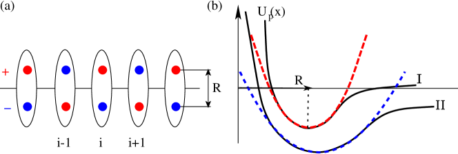
Figure 1: (a) Sketch of a 1D chain of polar molecules; (b) The potential of the pair with (II) or without (I) an extra charge carrier (full lines) is approximated by a polynomial (thick dashed lines)

The first model assumes that the carrier occupies an orbital of the ion with opposite charge. The attraction between them is then some constant, whereas the Coulomb repulsion between the carrier and the ion of like charge is $U(x_{i})=\frac{U_{0}n_{i}}{1-x_{i}/R}=U_{0}n_{i}\sum_{n=0}^{\infty}\left(\frac{x_{i}}{R}\right)^{n}$ where $n_{i}=1(n_{i}=0)$ if the carrier is (is not) present and $U_{0}>0$ is the characteristic energy. Using $x_{i}=\sqrt{\frac{\hbar}{2\mu\Omega}}(b_{i}+b_{i}^{\dagger})$ where $\mu$ is the reduced mass of the molecule, and truncating the series at $n=4$ leads to:

$${\cal H}_{\rm el-ph}=\sum_{n=1}^{4}{\cal H}_{\rm el-ph}^{(n)}=\sum_{n=1}^{4}g_{n}\sum_{i}c_{i}^{\dagger}c_{i}(b_{i}+b_{i}^{\dagger})^{n},$$ (1)

where $g_{n}=g_{1}\zeta^{n-1}$ with $\zeta=A/R$ and $A=\sqrt{\hbar/(2\mu\Omega)}$ the zero-point amplitude of the harmonic oscillator.

The second model assumes that the carrier is an electron (hole) that occupies an anti-bonding (bonding) orbital of the molecule; all bonding orbitals are initially full since the parent crystal is an insulator. In both cases the energy increases by an overlap integral which decreases exponentially with the distance: $U(x_{i})\sim n_{i}e^{-\frac{R-x_{i}}{a_{B}}}$ where $a_{B}$ is the Bohr radius. A Taylor expansion to fourth order in $x_{i}$ leads again to Eq. (1) but now $g_{n}/g_{1}=2^{n-1}\zeta^{n-1}/n!$ for $\zeta=g_{2}/g_{1}=A/(2a_{B})$, where again $A=\sqrt{\hbar/(2\mu\Omega)}$.

We define as the linear model the case where only $g_{1}\neq 0$ (i.e., the usual Holstein model); as the quadratic model the case where only $g_{1}\neq 0,g_{2}\neq 0$; and as the quartic model the case where all $g_{n}\neq 0$. The case with only $g_{4}=0$ is not considered because it is unstable.

The linear Holstein model is characterized by two dimensionless parameters: the effective coupling strength $\lambda=g_{1}^{2}/(2dt\Omega)$, where $d$ is the dimension of the lattice, and the adiabaticity ratio $\Omega/(4dt)$. As long as the latter is not very small, the former controls the phenomenology, with the crossover to small polaron physics occurring for $\lambda\sim 1$ [16]. For ease of comparison, we continue to use these parameters when characterizing the higher order models. For the quadratic model, the new energy scale $g_{2}$ results in a third dimensionless parameter $\zeta=g_{2}/g_{1}$. For the quartic model there are two more parameters $g_{n}/g_{1}$, $n=3,4$. Both scale like $\zeta^{n-1}$ but with different prefactors. We use $g_{n}/g_{1}=\zeta^{n-1}$ like in the first model since for the second model the prefactors are less than 1, making these terms smaller and thus less important.

For specificity, from now we assume $\zeta>0$ ($\zeta<0$ is briefly discussed at the end). As we show below, in this case we find that while quadratic terms are important when the linear coupling is large, addition of the $n=3,4$ terms only leads to small quantitative changes and can be ignored. This justifies a posteriori why we do not include anharmonic corrections in ${\cal H}_{\rm ph}$ and/or higher order terms with $n>4$ in the electron-phonon coupling.

We now describe in detail the MA solution for the quadratic model. The calculations for the quartic model are analogous but much more tedious.

We want to find the single particle Green’s function $G(\vect{k},\omega)=\braket{0}{c^{\phantom{\dagger}}_{\vect{k}}\hat{G}(\omega)c^{\dagger}_{\vect{k}}}{0}$ where $\hat{G}(\omega)=[\omega-\mathcal{H}+i\eta]^{-1}$ is the resolvent for this Hamiltonian, with $\eta\rightarrow 0$ a small positive number and $\ket{0}$ the vacuum state. From this we can extract all the polaron’s GS properties [14]. We rewrite the quadratic Hamiltonian as $\mathcal{H}=\mathcal{H}_{0}+\mathcal{H}_{1}$, where $\mathcal{H}_{0}={\cal H}_{\rm el}+{\cal H}_{\rm ph}+g_{2}\sum_{i}c_{i}^{\dagger}c_{i}^{\phantom{\dagger}}\left(2b_{i}^{\dagger}b_{i}^{\phantom{\dagger}}+1\right)$ while $\mathcal{H}_{1}=\sum_{i}c_{i}^{\dagger}c_{i}^{\phantom{\dagger}}\left[g_{1}(b_{i}^{\dagger}+b_{i}^{\phantom{\dagger}})+g_{2}(b_{i}^{\dagger 2}+b_{i}^{2})\right].$ The equation of motion (EOM) for the propagator is obtained recursively from Dyson’s identity, $\hat{G}(\omega)=\hat{G}_{0}(\omega)+\hat{G}(\omega)\mathcal{H}_{1}\hat{G}_{0}(\omega)$ where $\hat{G}_{0}(\omega)=[\omega-\mathcal{H}_{0}+i\eta]^{-1}$ is the resolvent for ${\cal H}_{0}$. Using it in $G(\vect{k},\omega)$ yields the EOM

$$G(\vect{k},\omega)=G_{0}(\vect{k},\omega)\left[1+\sum_{n=1}^{2}\sum_{i}\frac{e^{i\vect{k}\cdot\vect{r}_{i}}}{\sqrt{N}}g_{n}F_{n}(\vect{k},\omega;i)\right]$$ (2)

where $F_{n}(\vect{k},\omega;i)=\braket{0}{c^{\phantom{\dagger}}_{\vect{k}}\hat{G}(\omega)c_{i}^{\dagger}(b_{i}^{\dagger})^{n}}{0}.$

Applying Dyson’s identity to generate EOM for the $F_{n}$ propagators results in an infinite system of coupled equations which involves many other generalized propagators. MA [14, 15] circumvents this complication by making the approximation $G_{0}(i-j,\omega;n)\approx\delta_{ij}\bar{g}_{0}(\omega;n)$ for any $n\geq 1$, where $G_{0}(i-j,\omega;n)=\frac{1}{n!}\braket{0}{c_{i}^{\phantom{\dagger}}b_{i}^{n}\hat{G}_{0}(\omega)(b_{i}^{\dagger})^{n}c_{i}^{\dagger}}{0}$. This is justified because the polaron GS energy lies below the free particle spectrum, and for such energies the free-particle propagator decreases exponentially with $|i-j|$. Thus, MA keeps the largest contribution and ignores the exponentially smaller ones. This becomes exact in the strong-coupling limit $t\rightarrow 0$. The propagator $\bar{g}_{0}(\omega;n)=\left[1/\tilde{g}_{0}(\omega-n\Omega-g_{2})-2g_{2}n\right]^{-1}$ is that of a carrier scattered by an on-site potential $2g_{2}n$, where $\tilde{g}_{0}(\omega)=\frac{1}{N}\sum_{\vect{k}}1/(\omega-\epsilon_{\vect{k}}+i\eta)$.

MA allows us to obtain a simplified hierarchy of EOM involving only the generalized Green’s functions $F_{n}$. For any $n\geq 1$, they read:

$$F_{n}(\vect{k},\omega;i)=\bar{g}_{0}(\omega;n)\cdot\big{[}n(n-1)g_{2}F_{n-2}(\vect{k},\omega;i)$$

$$+ng_{1}F_{n-1}(\vect{k},\omega;i)+g_{1}F_{n+1}(\vect{k},\omega;i)+g_{2}F_{n+2}(\vect{k},\omega;i)\big{]}.$$

Since the arguments of all $F_{n}$ propagators are the same, we suppress them in the following for simplicity.

Following the technique introduced in Ref. [17], we reduce this to a simple recursive relation for the vector $\vect{W_{n}}=(F_{2n-1},F_{2n})$. The EOM for $\vect{W_{n}}$ are $\tens{\gamma_{n}}\vect{W_{n}}=\tens{\alpha_{n}}\vect{W_{n-1}}+\tens{\beta_{n}}\vect{W_{n+1}},$ where the $\tens{\alpha_{n}}$, $\tens{\beta_{n}}$ and $\tens{\gamma_{n}}$ are $2\times 2$ matrices whose coefficients are read off of the EOM, namely $\tens{\alpha_{n}}|_{11}=(2n-1)(2n-2)g_{2}\bar{g}_{0}(\omega;2n-1)$, $\tens{\alpha_{n}}|_{12}=(2n-1)g_{1}\bar{g}_{0}(\omega;2n-1)$, $\tens{\alpha_{n}}|_{21}=0$ and $\tens{\alpha_{n}}|_{22}=2n(2n-1)g_{2}\bar{g}_{0}(\omega;2n)$, while

$$\tens{\beta_{n}}=\begin{pmatrix}g_{2}\bar{g}_{0}(\omega;2n-1)&0\\ g_{1}\bar{g}_{0}(\omega;2n)&g_{2}\bar{g}_{0}(\omega;2n)\end{pmatrix},$$ (3)

$$\tens{\gamma_{n}}=\begin{pmatrix}1&-g_{1}\bar{g}_{0}(\omega;2n-1)\\ -2ng_{1}\bar{g}_{0}(\omega;2n)&1\end{pmatrix}.$$ (4)

This simple recursive relation for $\vect{W_{n}}$ has the solution $\vect{W_{n}}=\tens{A_{n}}\vect{W_{n-1}}$ for any $n\geq 1$, where $\tens{A_{n}}$ are $2\times 2$ matrices obtained from the infinite continued fraction

$$\tens{A_{n}}=\left[\tens{\gamma_{n}}-\tens{\beta_{n}}\tens{A_{n+1}}\right]^{-1}\tens{\alpha_{n}}.$$ (5)

In practice, we start with $A_{N}=0$ for a sufficiently large cutoff $N$, chosen so that the results are insensitive to further increases in it ($N\sim 100$ is usually sufficient).

We find $\tens{A_{1}}=\begin{pmatrix}0&a_{12}\\ 0&a_{22}\end{pmatrix}$, where $a_{12}$ and $a_{22}$ are obtained after using Eq. (5) $N-1$ times. As a result, $F_{1}=a_{12}F_{0}$, $F_{2}=a_{22}F_{0}$, where $G(\vect{k},\omega)=\sum_{i}e^{i\vect{k}\cdot\vect{r}_{i}}/\sqrt{N}F_{0}(\vect{k},\omega;i)$. Using these in Eq. (2) leads to a solution of the expected form $G(\vect{k},\omega)=\left[\omega-\epsilon_{\vect{k}}-\Sigma(\omega)+i\eta\right]^{-1}$, with the MA self-energy for the quadratic model: $\Sigma(\omega)=g_{1}a_{12}(\omega)+g_{2}a_{22}(\omega)$.

The reason why the self-energy is local at this level of MA is the simplicity of this Hamiltonian, whose vertices are momentum independent; this issue is discussed at length for the linear Holstein model in Ref. [15].

The quartic model is solved analogously. The main difference is that here the EOM for $F_{n}$ involves 9 consecutive terms, from $F_{n-4}$ to $F_{n+4}$. These can also be rewritten as simple recurrence relations $\tens{\gamma_{n}}\vect{W_{n}}=\tens{\alpha_{n}}\vect{W_{n-1}}+\tens{\beta_{n}}\vect{W_{n+1}},$ but now $\tens{\alpha_{n}}$, $\tens{\beta_{n}}$ and $\tens{\gamma_{n}}$ are $4\times 4$ matrices. Their expressions are too long to be listed here.

3 Results and Discussion

To gauge the relevance of the higher-order el-ph coupling terms we plot in Fig. 2 the evolution with $\zeta$ of a polaron property that can be directly measured, namely the quasiparticle weight $Z=m/m^{*}$ where $m,m^{*}$ are the carrier and the polaron mass, respectively. We also show the average phonon number $N_{ph}$. The results are for a one-dimensional chain. Results in higher dimensions are qualitatively similar to these 1D results for small $\lambda$, and become quantitatively similar to them in the interesting regime of large $\lambda$ where all of them converge towards those of the atomic limit $t=0$.

First, we note that the $\zeta=0$ intercepts trace the predictions of the linear model: with increased coupling $\lambda$, $Z$ decreases while $N_{ph}$ increases as the polaron acquires a robust phonon cloud [14, 16]. From these intercepts, we estimate that the linear model predicts the crossover to the small polaron regime to occur around $\lambda\sim 1.5$ for this adiabaticity ratio and dimension.

The quadratic model, whose predictions are indicated by lines, shows a very strong dependence of $\zeta$ for strong linear coupling $\lambda\geq 1.5$: here both $Z$ and $N_{ph}$ vary by about an order of magnitude as $\zeta$ increases from 0 to $0.1$. For higher $\zeta$, $Z$ and $N_{ph}$ have a slight turnaround towards smaller/larger values, for reasons explained below, but are still consistent with a large polaron. These results indicate that the quadratic term can completely change the behavior of the polaron in the limit of medium and large $\lambda$. For example, in the quadratic model at $\lambda=1.5$ and $\zeta\sim 0.1$ the polaron is light and with a small phonon cloud, in total disagreement with the linear model prediction of a heavy small polaron at this $\lambda$.

Of course, this raises the question of how large $\zeta$ is. The answer is material specific, but as an extreme case, let H₂ be the unit of the molecular crystal. This case is described by model two, so $\zeta\sim 2A/a_{B}$, where $a_{B}\approx 0.5\AA$ while $A\approx 0.1\AA$ if we use $\Omega\approx 0.5eV$ appropriate for a H₂ molecule [18]. This leads to a very large $\zeta\sim 0.4$. Other atoms are heavier but phonon frequencies are usually much smaller than $0.5eV$, so it is not clear whether $A\sim 1/\sqrt{\mu\Omega}$ changes much. The Bohr radius (or distance $R$ between atoms, for model 1) is usually larger than $0.5\AA$ but not by a lot, maybe up to a factor 5 for $R$; thus we expect smaller $\zeta$ in real materials but the change is likely not by orders of magnitude. Fig. 2 shows that values as small as $\zeta\sim 0.05$ already lead to significant quantitative changes in $m^{*}$.

Inclusion of cubic and quartic terms (the symbols show the results of the quartic model) further changes $Z$ and $N_{ph}$, but these changes are much smaller for all $\zeta$, of up to $\sim 10\%$ when compared to the quadratic model values, as opposed to order of magnitude changes between the quadratic and the linear models. Thus, these terms are much less relevant and can be ignored without losing much accuracy. As discussed, their small effect explains why we do not consider terms with even higher order $n$, nor $n=4$ anharmonic terms in the phonon Hamiltonian.

[width=0.95]fig2.eps

Figure 2: GS quasiparticle weight (left panel) and GS average phonon number (right panel) vs. $\zeta$, in the quadratic ($n=2$, lines) and quartic ($n=4$, symbols) models, for various values of $\lambda$ and $\Omega=0.5t$, in one dimension.

To understand the effects of the quadratic term at large $\lambda$, we study it in the atomic limit $t=0$ ($\lambda=\infty$) where the carrier remains at one site and interacts only with the phonons of that site. Focusing on this site, its quadratic Hamiltonian ${\cal H}^{(2)}_{\rm at}=\Omega b^{\dagger}b+\sum_{n=1}^{2}g_{n}(b^{\dagger}+b)^{n}$ is well-studied in the field of quantum optics, where it describes so-called squeezed coherent states [19]. The extra charge changes the origin and spring constant of the original harmonic oscillator which means that the Hamiltonian is easily diagonalized by changing to new bosonic operators $\gamma^{\dagger}=ub^{\dagger}+vb+w$, where $u$, $v$ and $w$ are such that $\mathcal{H}^{(2)}_{\rm at}=\Omega_{\rm at}\gamma^{\dagger}\gamma+E^{(\text{at})}_{GS}$. We find $\Omega_{\rm at}=\sqrt{\Omega(\Omega+4g_{2})}$, $u=\sqrt{\left(\Omega+2g_{2}+\Omega_{\text{at}}\right)/(2\Omega_{\text{at}})}$, $w=g_{1}\sqrt{\Omega/\Omega_{\text{at}}^{3}}$ and $v=\mathrm{sgn}(g_{2})\sqrt{\left(\Omega+2g_{2}-\Omega_{\text{at}}\right)/(2\Omega_{\text{at}})}$. From these, we obtain $E_{\text{GS}}^{\text{at}}=-\frac{g_{1}^{2}\Omega}{\Omega_{\text{at}}^{2}}+\frac{1}{2}(\Omega_{\text{at}}-\Omega)$, $N_{\text{ph}}^{(\text{at})}=\frac{1}{2}\left[\frac{\Omega+2g_{2}}{\Omega_{\text{at}}}-1\right]+\frac{g_{1}^{2}}{(\Omega+4g_{2})^{2}}$ and $Z_{\rm at}=\frac{1}{u}\exp\left[-w^{2}\left(1-\frac{v}{u}\right)\right]$. The latter result requires the expansion of the squeezed coherent states in the number state basis [20].

Figure 3 shows $Z_{\rm at}$ and $N^{(\text{at})}_{\text{ph}}$ vs. $\zeta$ (thick lines), which agree well with the corresponding $\lambda=2$ results of Fig. 2. In particular, for $\zeta\rightarrow 0$ we find $\Omega_{\rm at}=\Omega+2g_{1}\zeta+{\cal O}(\zeta^{2})$, $N_{\text{ph}}^{(\text{at})}=\frac{g_{1}^{2}}{\Omega^{2}}\left[1-{\frac{8g_{1}}{\Omega}\zeta+\mathcal{O}}(\zeta^{2})\right]$, explaining their linear increase/decreases for small $\zeta$.

[width=]fig3.eps

Figure 3: (left) $Z_{\rm at}$, and (right) $N^{(\text{at})}_{\text{ph}}$ vs. $\zeta$, for $g_{1}=\sqrt{2}$ and $\Omega=0.5$ (full lines). Dashed lines show the mean-field estimates, while the dot-dashed lines show the results of fitting $\tilde{g}/\tilde{\Omega}$ to exactly reproduce the other quantity. See text for more details.

The slight turnaround of the $Z$ and $N_{\text{ph}}$ curves at larger values of $\zeta$ is also observed in the atomic limit of the quadratic model. The reason is that the first term in $N_{\text{ph}}^{\text{(at)}}$ increases whereas the second term decreases with $\zeta$. As discussed above, for small $\zeta$ the second term dominates and the overall number of phonons decreases. For large $\zeta$, however, the second term vanishes whereas the first term diverges as $\sqrt{g_{2}}=\sqrt{\zeta g_{1}}$. Hence, as $\zeta$ increases $N_{\text{ph}}^{\text{at}}$ has a minimum, and then starts to increase with $\zeta$. Basically, here the $g_{2}(b^{\dagger 2}+b^{2})$ coupling dominates over the linear coupling $g_{1}(b^{\dagger}+b)$ and changes the trend.

This leads us to pose the question whether these exact results of the quadratic atomic model can be fit well by an effective linear model ${\cal H}^{(1)}_{\rm at}=\tilde{\Omega}b^{\dagger}b+\tilde{g}(b^{\dagger}+b)$, for some appropriate choice of the effective parameters $\tilde{\Omega},\tilde{g}$. One way to achieve this is with a mean-field ansatz $b^{\dagger 2}\approx 2\langle b^{\dagger}\rangle b^{\dagger}-\langle b^{\dagger}\rangle^{2}$, with $\langle b^{\dagger}\rangle$ the GS expectation value of $b^{\dagger}$. The self-consistency condition $\langle b^{\dagger}\rangle=-(g_{1}+2g_{2}\langle b^{\dagger}\rangle)/(\Omega+2g_{2})$ leads to the mean-field estimates $\tilde{\Omega}_{\rm MF}=\Omega+2g_{2}$, $\tilde{g}_{\rm MF}=g_{1}-2g_{1}g_{2}/(\Omega+4g_{2})$. Thus, for small $\zeta=g_{2}/g_{1}$, $\tilde{\Omega}_{\rm MF}$ increases whereas $\tilde{g}_{\rm MF}$ decreases with increasing $\zeta$ so the effective coupling $\tilde{\lambda}=\tilde{g}^{2}/(2dt\tilde{\Omega})$ decreases with $\zeta$. This is consistent with the observed move away from the small polaron limit with increasing $\zeta$. Quantitatively, however, these mean-field results (dashed lines in Fig. 3) are not very accurate for small $\zeta$, and fail to capture even qualitatively the correct behavior when $\zeta\gg 1$, since here $N^{(\text{at})}_{\text{ph}}\rightarrow\infty$ while $N_{\text{ph}}^{(MF)}=\tilde{g}_{\rm MF}^{2}/\tilde{\Omega}_{\rm MF}^{2}\rightarrow 0$.

In fact, there is no choice for effective linear parameters $\tilde{g}$ and $\tilde{\Omega}$ that reproduces the results of the quadratic model. This is because in the linear model, both $\tilde{Z}$ and $\tilde{N}_{\text{ph}}$ are functions of $\tilde{g}/\tilde{\Omega}$ only. Fig. 3 shows that if one chooses this ratio so that $N^{(\text{at})}_{\rm ph}=\tilde{N}_{\rm ph}$, then $\tilde{Z}$ (dot-dashed line in the left panel) disagrees with $Z_{\rm at}$, and vice versa. Even more significant is the fact that even if one could find a way to choose $\tilde{g},\tilde{\Omega}$ so that the overall agreement is satisfactory for all GS properties, the linear model’s prediction for higher energy features would still be completely wrong. For example, it would predict the polaron+one-phonon continuum to occur at $E_{GS}+\tilde{\Omega}$ instead of the proper $E_{GS}+\Omega$ threshold. Since in the atomic limit the predictions of the quadratic model cannot be reproduced with a renormalized linear model, we conclude that this must hold true at finite hopping $t$ as well, at least for large $\lambda$ where the quadratic terms are important.

So far we discussed moderate values of the adiabaticity ratio $\Omega/t=0.5$, as well as the anti-adiabatic (atomic) limit. MA predicts similar results in the adiabatic limit $\Omega/t\rightarrow 0$ for large $\lambda$, where it remains accurate, but is unsuitable to study small and moderate couplings [15]. We expect that here the quadratic coupling is essential even for small couplings $\lambda\rightarrow 0$, because the term $2g_{2}\sum_{i}b_{i}^{\dagger}b_{i}$ insures that phonons are gapped even though $\Omega=0$.

So far we also only discussed the case $\zeta>0$. The behavior of models with $\zeta<0$ can be glimpsed at from the exact results in the atomic limit. For small negative $\zeta$, the results listed above show that the average phonon number $N_{\text{ph}}^{\text{(at)}}$ increases with $|\zeta|$ while the qp weight $Z_{\rm at}$ decreases fast, i.e. the polaron moves more strongly into the small polaron limit. This is in agreement with the MA predictions for the quadratic model (not shown). Here, however, we must limit ourselves to values $|\zeta|<\Omega/(4g_{1})$ so that $\Omega_{\rm at}$ remains a real quantity (a similar threshold is found for the full quadratic model. Note that the value of this threshold decreases with increasing $\lambda$). For values of $|\zeta|$ above this threshold the quadratic model becomes unstable. This, of course, is unphysical. In reality, here one is forced to include higher order (anharmonic) terms in the phonon Hamiltonian ${\cal H}_{\rm ph}$ since they guarantee the stability of the lattice if the quadratic terms fail to do so. Such anharmonic terms may have little to no effect in the absence of the carrier, but clearly become important in its presence, in this limit. They can be treated with the same MA formalism we used here. Their effects, as well as a full analysis of all possible signs of the non-linearities and the resulting polaron physics will be presented elsewhere. For our current purposes, it is obvious that in the case $\zeta<0$, higher order terms in el-ph coupling also play a key role in determining the polaron properties unless $\lambda$ is very small, and therefore cannot be ignored.

The results presented so far clearly demonstrate the importance of non-linear el-ph coupling terms if the linear coupling $\lambda$ is moderate or large, through their significant effects on the properties of a single Holstein polaron.

A reasonable follow-up question is whether such dramatic effects are limited to the single polaron limit or are expected to extend to finite carrier concentrations. While the limit of large carrier concentrations remains to be investigated in future work, here we present strong evidence that quadratic terms are likely to be equally important at small but finite carrier concentrations.

Of course, for finite carrier concentrations one needs to supplement the Hamiltonian with a term describing carrier-carrier interactions. The simplest such term is an on-site Hubbard repulsion ${\cal H}_{U}=U\sum_{i}n_{i\uparrow}n_{i\downarrow}$, and gives rise to the Hubbard-Holstein Hamiltonian. The linear version of this Hamiltonian has been studied extensively by a variety of numerical methods [16]. In particular, for low carrier concentrations and focusing on the small polaron/bipolaron limit, the phase diagram has been shown to consist of three regions: (i) for large $\lambda$ and small $U$, the deformation energy favors the formation of on-site bipolarons, also known as the $S_{0}$ bipolarons; (ii) increasing $U$ eventually makes having two carriers at the same site too expensive, and the $S_{0}$ bipolarons evolve into weakly-bound $S_{1}$ bipolarons, where the two carriers sit on neighboring sites. The binding is now provided by virtual hopping processes which allow each carrier to interact with the cloud of its neighbor. However, at smaller $\lambda$ and larger $U$ this binding mechanism is insufficient to stabilize the S1 bipolaron, and instead one finds (iii) a ground state consisting of unbound polarons.

[width=]fig4.eps

Figure 4: Estimate of the bipolaron phase diagram in 1D for $\Omega/t=0.5$ and for different values of $\zeta$, based on second order perturbation theory in $t$. In all four panels, the solid lines show the transition from $S_{0}$ (on-site) stable bipolarons to $S_{1}$ (nearest-neighbor) stable bipolarons, while the dashed lines show the unbinding transition above which bound polarons are unstable. Note that panels (c) and (d) have a significantly rescaled $y$-axis. See text for more details.

This phase diagram has been found numerically in 1D [21] and 2D [22] for the linear Hubbard-Holstein model. Some results in 3D have also become available very recently [23]. In 1D and 2D, the separation lines between the various phases are found to be close to those estimated using second order perturbation theory in the hopping $t$, starting from the atomic limit [21, 22]. This is expected since for large linear coupling $\lambda$, the results always converge toward those predicted by the atomic limit.

Since the quadratic Hamiltonian can be diagonalized exactly in the atomic limit, we use second order perturbation theory to estimate the location of the separation lines for various values of $\zeta>0$. The results are shown in Fig. 4. Panel (a) shows the rough phase diagram for $\zeta=0$, in agreement with the asymptotic estimates shown in Refs. [21, 22] (note that the definition of the effective coupling used in those works differs by various factors from our definition for $\lambda$). Panels (b)-(d) show a very significant change with increasing $\zeta$. Even the presence of an extremely small quadratic term $\zeta=0.01$ moves the two lines to considerably lower $U$ values, as shown in panel (b), while for $\zeta=0.05$ and $0.1$, the bipolarons are stable only in a very narrow region with small values of $U$ (note that the vertical axes are rescaled for panels (c) and (d)).

The dramatic change with increasing $\zeta$ in the location of these asymptotic estimates for the various bipolaron transitions/crossovers strongly suggests that non-linear el-ph coupling terms remain just as important in the limit of small carrier concentrations as they have been shown to be in the single polaron limit. In particular, these results suggest that the presence of non-linear el-ph coupling terms leads to a significant suppression of the phonon-mediated interaction between carriers, so that the addition of a small repulsion $U$ suffices to break the bipolarons into unbound polarons (whose properties are also strongly affected by the non-linear terms, as already shown).

The Holstein model is the simplest example of a $g(q)$ model, i.e. a model where the electron-phonon interaction depends only on the momentum of the phonon. Physically, such models appear when the coupling to the lattice manifests itself through a modulation of the on-site energy of the carrier. The Fröhlich model is another famous example of $g(q)$ coupling. Models of this type are found to have qualitatively similar behavior, with small polarons forming when the effective coupling increases. These small polarons always have robust clouds, with significant distortions of the lattice in their vicinity. We therefore expect that non-linear terms become important for all such models at sufficiently large linear coupling.

To summarize, we have shown that non-linear terms in the el-ph coupling must be included in a Holstein model if the linear coupling is large enough to predict small polaron formation, and that doing so may very significantly change the results. We also argued that these changes cannot be accounted for by a linear Holstein model with renormalized parameters. These results show that we have to (re)consider carefully how we model interactions with phonons (more generally, with any bosons) in materials where such interactions are expected to be strong, at least for low carrier concentrations and for models where this coupling modulates the on-site energy of the carriers. Whether this is also true in the metallic regime and/or for other types of models remains an open question.

- [1] \NameMatsui H., Mishchenko A. S. Hasegawa T. \REVIEWPhys. Rev. Lett.1042010056602; \NameCiuchi S. Fratini S. \REVIEWPhys. Rev. Lett.1062011166403.
- [2] \NameLanzara A. et al. \REVIEWNature4122001510; \NameShen K. et al. \REVIEWPhys. Rev. Lett.932004267002; \NameReznik D. et al. \REVIEWNature44020061170; \NameLee J. et al. \REVIEWNature4422010546; \NameGadermaier C. et al. \REVIEWPhys. Rev. Lett.1052010257001 \NameGunnarsson O. Rösch O. \REVIEWJ. Phys. Condens. Matter202008043201.
- [3] \NameMannella N. et al. \REVIEWNature4382005474
- [4] \NameYildirim T. et al. \REVIEWPhys. Rev. Lett.872001037001; \NameLiu A. Y., Mazin I. I. Kortus J. \REVIEWPhys. Rev. Lett.872001087005; \NameMazin I. I. Antropov V. \REVIEWPhysica. C. Supercond.385200349; \NameChoi H. J. et al. \REVIEWNature4182002758.
- [5] \NameKaminski A. et al. \REVIEWPhys. Rev. Lett.8620011070; \NameKim T. K. et al. \REVIEWPhys. Rev. Lett.912003167002.
- [6] \NameVeenstra C. N.,Goodvin G. L., Berciu M. Damascelli A. \REVIEWPhys. Rev. B842011085126.
- [7] \NameHolstein T. \REVIEWAnn. Phys.81959325.
- [8] \NameFröhlich H. \REVIEWAdv. Phys.31954325.
- [9] \NameMishchenko A. S. Nagaosa N. \REVIEWPhys. Rev. Lett.932004036402; \NameMishchenko A. S. et al. \REVIEWPhys. Rev. Lett.1002008166401 and references therein.
- [10] \NameHerrera F. Krems R. V. \REVIEWPhys. Rev. A842011051401; \NameHague J. P. MacCormick C. \REVIEWNew J. Phys.142012033019; \NameStojanovic V. M. et al. \REVIEWPhys. Rev. Lett.1092012250501; \NameHerrera F. et al. \REVIEWPhys. Rev. Lett.1102013223002;
- [11] \NameEntin-Wohlman O., Gutfreund H. Weger M. \REVIEWSolid. State. Comm.4619831; ibid \REVIEWJ. Phys. C Solid State Phys.181985L61.
- [12] \NameCrespi V.H., Cohen M.L. \REVIEWPhys. Rev. B481993398.
- [13] \NameKenkre V. M. \REVIEWPhys. D1131998233
- [14] \NameGoodvin G. L., Berciu M. Sawatzky G. A. \REVIEWPhys. Rev. B742006245104.
- [15] \NameBerciu M. Goodvin G. L. \REVIEWPhys. Rev. B762007165109.
- [16] \NameFehske H. Trugman S. A. \BookPolarons in Advanced Materials \EditorAlexandrov A. S. \PublCanopus, Bath/Springer-Verlag, Bath \Year2007 \Pages393461.
- [17] \NameMoeller M., Mukherjee A., Adolphs C. P. J., Marchand D. J. J. Berciu M. \REVIEWJ. Phys. A Math. Theor.452012115206.
- [18] \NameHerzberg G. \REVIEWPhys. Rev. Lett.2319691081.
- [19] \NameGerry C. C. Knight P. L. \BookIntroductory Quantum Optics \PublCambridge University Press \Year2005
- [20] \NameStoler D. \REVIEWPhys. Rev. D119703217; \SAME419701925; \NameYuen H. P. \REVIEWPhys. Rev. A1319762226.
- [21] \NameBonca J., Katrasnik T. Trugman S. A. \REVIEWPhys. Rev. Lett.8420003153; \NameBarisic O. S. Barisic S. \REVIEWEur. Phys. J. B852012111.
- [22] \NameMacridin A., Sawatzky G. A. Jarrell M. \REVIEWPhys. Rev. B692004245111.
- [23] \NameDavenport A. R., Hague J. P. Kornilovitch P. E. \REVIEWPhys. Rev. B862012035106.