Thermal noise for quantum state inference

Abstract

In this work we describe a simple and efficient scheme for inference of photon number distribution by adding variable thermal noise to the signal. The inference remains feasible even if the scheme parameters are subject to random dynamical change.

Quantum state tomography is the most advanced and complete diagnostic tool available now. It allows one inferring maximal possible information about the state of physical system or about the process all . Quantum tomography has already become a standard experimental tool enabling reconstruction even such fragile, exquisitely quantum objects as ”Schrodinger cats” Ourjoumtsev . Intuitively, one expects that for performing measurements able to collect information sufficient to reconstruct a quantum state or process, it is necessary to build rather precise measurement set-up. This intuition seems to be confirmed by existence of limits for detection efficiency required for performing a reconstruction, such as $50\%$ threshold for a quantum homodyne tomography vogel ; raymer . Moreover, it seems natural supposing that it is necessary to know precisely what exactly one’s measurement set-up detects (in more formal language, it is seems necessary to know all the elements of the positive valued operator measure, POVM, describing the experiment).

Well, recently some works have appeared giving a rather obvious hint: with quantum measurements it might be really unnecessary to struggle for achieving exactly known (i.e. calibrated), and perfectly controllable measurement set-up. Under certain quite general conditions (such as, for example, Gaussianity of the state is question) it is possible to update information about the set-up and the signal state simultaneously (which was termed ”self-calibration”) mogilevtsev2009 . Very recently experimental demonstrations of self-calibration were given branczyk2012 ; kulik . Moreover, it was demonstrated that sufficient knowledge about set-up can be acquired in the process of collecting data even in absence of any initial information about the measurement set-up our fresh njp .

However, self-calibrating approaches described above still suppose that there is some fixed measurement set-up, albeit possibly unknown one. But what if some noise is present? What if it is subjected to random (and possible uncontrollable) change? In this work we are demonstrating that classical noise affecting the measurement set-up can be beneficial and usable for building robust, efficient and simple measurement set-up (which can even be much simpler than exiting methods) for certain tomography tasks. Moreover, even randomly changing POVM parameters might be not an obstacle for these tasks.

A general impression about a possible role of noise can be given with the following simple example. Let us consider a set-up performing projection on the coherent state with the amplitude $\alpha$, i.e. with the POVM element $\Pi=|\alpha\rangle\langle\alpha|$ (which can be realized with heterodyne measurement yen ). If the amplitude $\alpha$ undergoes random changes (say, $\delta_{j}$) around some particular value, say, $\alpha_{0}$, for a sufficiently large number of different $\delta_{j}$ the resulting set of POVM elements (i.e. of the form $\Pi_{j}=|\alpha_{0}+\delta_{j}\rangle\langle\alpha_{0}+\delta_{j}|$) will be sufficient for performing a complete state/process reconstruction (which is attested by recent schemes of ”data pattern tomography” our fresh njp ; our prl 2010 and quantum process tomography lvovsky ). So, adding noise to a measurement can actually increase a region that the measurement set-up is actually ”seeing”, i.e. the search subspace.

Now let us demonstrate how noise can be implemented for devising simple and efficient set-up for inference of photon number distribution of a single-mode state of electromagnetic field. Notice that, for example, for quantum homodyne tomography an inference of photon number distribution is not much simpler than inferring the complete density matrix (one needs performing the same set of quadrature measurements). The task can be made easier by building the specific set of POVM elements,

$$\Pi_{j}=\sum\limits_{n=0}^{N}r_{n}|n\rangle\langle n|,$$ (1)

where $|n\rangle$ are Fock states with $n$ photons. In the end of 90-s it was demonstrated that implementing only a single bucket detector with a set of variable absorbers changing the efficiency of the detection it is possible to collect data sufficient for inferring the photon number distribution mog98 . For this set-up one has $r_{n}=(1-\eta)^{n}$, where $\eta$ is the efficiency of the detector. The method was realized experimentally paris . It was shown also that adding a coherent shift to the signal state it is possible to perform a complete tomography us . However, an experimental realization of the scheme remained rather challenging due to necessity to perform calibration of absorbers for signals of a few-photon level. To avoid this more sophisticated set-up was suggested and realized; there the signal travels along the fiber loop splitting on each pass, seeloop ; loopnew ).

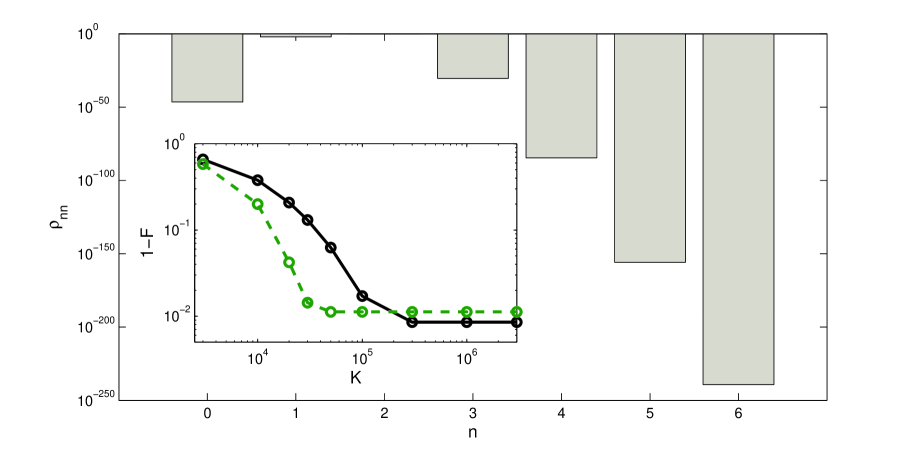
Figure 1: An example of two-photon Fock state maximal likelihood estimation using variable thermal noise. 30 values of average number,$\bar{n}$, of thermal photons were used equidistantly distributed in the interval [0.1,0.95]; the search space was from 0 to 12 photons, 10,000 iterations of the reconstruction algorithm were taken, starting with the maximal entropy state. The detector efficiency, $\eta$, is 0.8. The inset shows a dependence of fidelity on the number of iterations, $L$, for 20,000 measurements (solid line) and 10,000 measurements (dashed line) per each value of $\bar{n}$

Implementing noise gives a way to avoid using both sets of calibrated absorbers or loop detection for the task. Indeed, let us simply add a thermal noise (i.e. a source of detector ”dark counts”) with the average number of photons $\bar{n}$ to our signal. As follows from the Mandel’s formula, without the thermal noise mixed with the signal the probability to have no clicks on our bucket detector is given by

$$p(\eta)=\sum\limits_{n=0}(1-\eta)^{n}\rho_{nn},$$ (2)

where $\rho_{nn}$ are diagonal elements of the signal state density matrix in the Fock state basis; notice that $p(\eta)$ is, in fact, the photon-number generating function. When the thermal light with the average number of photons, $\bar{n}$, is added to the signal at the entrance of the detector, the probability (2) is modified as to perina ; rockower

$$p(\eta)\rightarrow p(\eta,\bar{n})=\frac{1}{1+\eta\bar{n}}p\left(\frac{\eta}{1+\eta\bar{n}}\right),$$ (3)

As it follows from Eq.(3), one can just mix thermal noises corresponding to different temperatures to build the POVM elements set required for inference of photon-number distribution. In Fig.1 an example of the two-photon Fock state reconstruction is given. For the task 30 different values of the average number of photons of the added thermal noise are taken. Efficient expectation-maximization iterative algorithm for maximal likelihood estimation was implemented us ; paris . For 10,000 measurements per each value of $\bar{n}$ a fidelity of more than 95$\%$ was reached for 10,000 iterations starting from the maximal entropy state. One should point out two important features of the suggested scheme. The first one is necessity to use rather large search subspace due to the photon-number distribution of the thermal state being long-tailed. The second one is the slower convergence of the algorithm for larger number of measurements (see inset in Fig.1). Increasing of the number of measurement ultimately is eventually leading to increase in the reconstruction accuracy. However, with larger number of measurements one can actually get worse results for the same number of iterations.

It should be stress out that adding thermal noise leads to significant simplification of the process of building the POVM elements set required for the reconstruction. Indeed, one is not even obliged to actually change parameters of the source of thermal noise; it is sufficient to change a time-window of detection to change effectively an average number of thermal photons. Notice, that thermal noise needs not to be pre-calibrated: it is possible to change noise temperature arbitrarily and calibrate it by temporarily switching off the signal and collecting data. It means that one can actually perform the reconstruction with usual daylight. The only obstacle is dispersion of the detection efficiency, so it is necessary to filter thermal noise to provide for the constant detector efficiency in the spectral interval of thermal noise and the signal.

Of course, when one tries to build set of POVM by adding noise, the question arises of its influence on possible reconstruction errors. Generally, the problem of error estimation for quantum tomography is rather ”hot” and controversial subject nowadays. Both method bases on ML estimation and Bayesian inference were suggested for the purpose (see, for example, Ref.cristandl and references therein). However, for diagonal elements inference with general POVM (1) we can suggest a simple estimation of error of the ML method along the lines suggested in Ref.mognjp (and somewhat in the spirit of approach used in Ref.cristandl ).

Let us consider our measurement with the general POVM (1) as the set of measurements with $K$ complete POVMs each having just two elements $\Pi_{j}$ and $I-\Pi_{j}$, $j=1,\ldots,K$. In the limit of large number $N_{j}\gg 1$ of runs with the $j$-th POVM of the set, the likelihood function has the following form

$$P(S_{1},S_{2},\ldots,S_{K}|\rho)$$

$$=\prod_{j=1}^{K}\frac{N_{j}!}{S_{j}!(N_{j}-S_{j})!}\mathrm{tr}(\Pi_{j}\rho)^{S_{j}}\mathrm{tr}([I-\Pi_{j}]\rho)^{N_{j}-S_{j}},\qquad$$ (4)

with the number of outcomes $S_{j}$ corresponding to the POVM element $\Pi_{j}$ (and, respectively, $N_{j}-S_{j}$ for $I-\Pi_{j}$), can be approximated by using the well-known large-$N$ limit of the binomial distribution (see, for instance, Ref. Gnedenko ). The latter is a Gaussian approximation, which in our case gives

$$P(S_{1},S_{2},\ldots,S_{K}|\rho)$$

$$\approx\prod_{j=1}^{K}\frac{1}{\sqrt{2\pi N_{j}}\sigma_{j}}\exp\left\{-N_{j}\frac{\left[\frac{S_{j}}{N_{j}}-\mathrm{tr}(\rho\Pi_{j})\right]^{2}}{2\sigma_{j}^{2}}\right\},$$ (5)

with

$$\sigma^{2}_{j}=\mathrm{tr}([I-\Pi_{j}]\rho)\mathrm{tr}(\Pi_{j}\rho).$$

For sufficiently large $N_{j}$ the width of the peak around the maximum likelihood point, i.e. the admissible values for $\rho_{mm}$, $m=0,1,\ldots,M$, is given by the variance appearing in Eq. (5). Therefore, the error $\delta$ for each $\rho_{mm}$ of the maximum likelihood estimate is on the order

$$\delta\sim\mathrm{max}\frac{\sigma_{j}}{\sqrt{N_{j}}}=\mathrm{max}\left\{\sqrt{\frac{S_{j}}{N^{2}_{j}}(1-\frac{S_{j}}{N_{j}})}\right\}.$$ (6)

An example of maximal error estimation for the two-photon Fock state reconstruction is shown in Fig. 2(b). One can see that Eq.(6) gives rather reasonable estimate of a maximal error for different number of measurements.

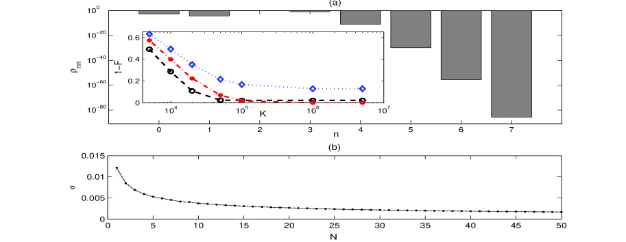
Figure 2: An example of two-photon Fock state maximal likelihood estimation using random variable thermal noise (a). The noise was taken to be Gaussian; 30 values of average number,$\bar{n}$, of thermal photons were used equidistantly distributed in the interval [0.1,0.95]; the variance is 0.1; the search space was from 0 to 12 photons, 1,000,000 iterations of the reconstruction algorithm were taken, starting with the maximal entropy state. The detector efficiency, $\eta$, is 0.8; the number of measurements is 50,000 per each value of $\bar{n}$. The inset shows a dependence of fidelity on the number of iterations, $K$, for 50,000 measurements and variance 0.1 (dash-dotted line); 10,000 measurements and variance 0.01 (dashed line); 10,000 measurements and variance 0.1 (dotted line) per each value of $\bar{n}$. The panel (b) shows an estimation of maximal errors made according to Eq.(6) for different number of trials, $N\times 1000$ per average value (solid line with dot marks), in comparison with the estimation for non-random POVM for fixed noise values equal to average ones. For this figure the average number of thermal photons is $\bar{n}=0.1$; the variance is 0.1; the search space was from 0 to 12 photons (dotted line).

The most obvious prerequisite for the ”thermal noise” reconstruction discussed above seems to be a constant predefined level of the noise. However, it is not hard to see that noise can be varied during the data collecting process. It can be even random. Indeed, if the set of parameters, $\vec{\mu}$, describing a particular POVM element in Eq.(1), $\Pi(\vec{\mu})$, represents a continuous random variable, then for the probability one has simply

$$p=\sum\limits_{n=0}[\bar{r}]_{n}\rho_{nn},\quad[\bar{r}]_{n}=\int d\vec{\mu}[r(\vec{\mu})]_{n},$$ (7)

Of course, for each run of the experiment the result will depend on the particular value of random parameters, $\vec{\mu}$. The reconstruction procedure hinges on the fact that for the sufficiently long sequence of trials one can assume the all results were obtained with the averaged POVM elements (7). For our example of the ”thermal noise” reconstruction these average POVM elements are to be defined on the calibration stage preceding a measurement of the state mixed with noise. Fig.2(a) demonstrates that the reconstruction with ”noisy” POVM elements is indeed feasible. There an example of two-photon state inference is shown for the ”thermal noise” reconstruction scheme with average number of photons fluctuating with the normal distribution. It is remarkable that one is able to achieve quite accurate reconstruction results with rather strong noise (when the variance of noise is comparable with the average value of $\bar{n}$). The pay-off is the necessity to increase the number of measurements per assumed averaged POVM element. However, this increase is not crucial (for instance, just five times for the example shown in Fig.2, corresponding to quite large variance of the noise). An estimation (6) shows that even for moderate number of trials maximal errors for fixed thermal noise and random one can be quite close (this situation is illustrated in the Fig.2(b)). Also, as the inset in Fig.2 demonstrates, random variation of the thermal noise do not noticeably worsen convergence of the reconstruction procedure in comparison with the ”fixed noise” results shown in Fig.1.

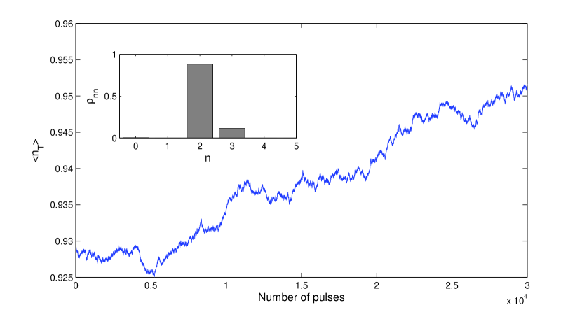
Figure 3: An example of a realization of the randomly changing average number of thermal photons. Random change is 1D random walk with probability 0.51 of jumping to a higher value of $\bar{n}$ (they are taken to be a discrete set with the step $5*10^{-4}$. The total of $9*10^{8}$ measurements were assumed. For the purpose of the reconstruction this set was divided on 30 subsets with 30,000 measurements in each. So, 30 different POVM elements (2) were assumed for the reconstruction with different $\bar{n}$ corresponding to averages over each subset. $10^{6}$ steps of the iteration procedure were takes. The inset shown the convergent result of the estimation of the signal two photon state.)

So, we have established that random variations around some fixed values of POVM parameters do not spoil the reconstruction. Now let us demonstrate that we can relax our requirement for controlling the experiment even further. Values of POVM parameters might be not fixed at all. A knowledge of average values of these parameters in a certain time interval is sufficient for performing the reconstruction. In Fig.3 an example of the reconstruction is shown for the average number of photons of the mixed thermal state undergoing the stochastic drift process. Since copies of the signal are assumed to be generated as an equidistant sequence of pulses, random change of the average number of photons was taken to be described as 1D random walk process. Probability of jump to higher $\bar{n}$ was taken to be slightly larger, than to lower $\bar{n}$ ($1\%$ higher), so the average number of photons was gradually increasing (see Fig.3). Consequent sets of 30,000 measurements were taken for averaging and assigning an averaged POVM element (whole of 30 different values of $\bar{n}$ non-equdistantly distributed in the interval [0.1,0.952]). As it can be seen in Fig.3, this approximation has allowed to achieve rather good estimation of the two-photon signal state even with rather moderate number of measurements.

Concluding: we have established that noising the measurement (or adding noise to the signal) can be a simple and efficient way to produce a set of POVM elements sufficient for reconstructing the state of the signal. Mixing the signal with the thermal noise on the detector (i.e. adding ”dark counts”), one can make very simple and non-expensive set-up for estimating a photon number distribution. One does not require for it a set of calibrated absorbers or loop detectors. Calibration of the thermal noise can be done directly in the process of measurement. Randomness of the added noise does not spoil the reconstruction, provided that the average values of noised parameters are known for sufficiently long series of trials. We have demonstrated that both for random parameters fluctuations around some set of fixed values, and for the random change similar to stochastic drift/random walk. The latter feature hints at the possibility to overcome the main reason of using the same source for generating the supposedly unknown signal and the reference field in the schemes of complete quantum tomography: the phase drift. Thus, this work is the step to reaching the ultimate goal of a quantum state tomography: accomplishing the reconstruction of truly unknown signal state.

The authors are thankful for Prof. Jan Perina for fruitful discussions. This work was supported by Foundation of Basic Research of the Republic of Belarus, by the National Academy of Sciences of Belarus through the Program ”Convergence”, by the Brazilian Agency FAPESP (project 2011/19696-0) (D.M.); and has received funding from the European Community’s Seventh Framework Programme (FP7/2007-2013) under grant agreement n^∘ 270843 (iQIT) (N.K.).

References

- (1) M. G. A. Paris and J. Řeháček (Eds), Quantum states estimation, Lect. Notes Phys. vol. 649 (Springer, Berlin Heidelberg, 2004).
- (2) A. Ourjoumtsev, R. Tualle-Brouri, J. Laurat, P. Grangier, Science 312, 83 (2006).
- (3) K. Vogel and H. Risken, Phys. Rev. A40, 2847 (1989).
- (4) D. T. Smithey, M. Beck, M. G. Raymer, and A. Faridani, Phys. Rev. Lett. 70, 1244 (1993).
- (5) D. Mogilevtsev, J. Rehacek, and Z. Hradil, Phys. Rev. A 79, (2010) 02010(R); D. Mogilevtsev, Phys. Rev. A 82, (2010) 021807(R); D. Mogilevtsev, J. Rehacek, and Z. Hradil, New J.Phys. 14, (2012) 095001.
- (6) A. M. Branczyk, D. H. Mahler, L. A. Rozema, A. Darabi, A. M. Steinberg and D. F. V. James, New J.Phys. 14, 085003 (2012).
- (7) S. Straupe, D. Ivanov, A. Kalinkin, I. Bobrov, S. P. Kulik, D. Mogilevtsev, arXiv:1112.3806v2 (2013).
- (8) D. Mogilevtsev, A. Ignatenko, A. Maloshtan, B. Stoklasa, J. Rehacek and Z. Hradil, Data pattern tomography: reconstruction with unknown apparatus, to appear in New J. Phys. (2013).
- (9) H. P. Yuen and J. H. Shapiro, IEEE Trans. Inf. Theory 24, 657 (1978); 25, 179 (1979).
- (10) J. Rehacek, D. Mogilevtsev, and Z. Hradil, Phys. Rev. Lett. 105, 010402 (2010).
- (11) M. Lobino, D. Korystov, C. Kupchack, E. Figueroa, B. C. Sanders and A. I. Lvovsky, Science 322 563(2008); S. Rahimi-Keshari, A. Scherer, A. Mann, A. T. Rezakhani, A. I. Lvovsky and B. C. Sanders, New J. Phys. 13 013006 (2011).
- (12) D. Mogilevtsev, Opt. Comm. 156, 307 (1998); D. Mogilevtsev, Acta Physica Slovaca 49, 743 (1999).
- (13) A.R. Rossi, S. Olivares, M.G.A. Paris, Phys. Rev. A 70, 055801 (2004); A.R. Rossi and M.G.A. Paris, Eur. Phys. J. D 32, 223 (2005); G. Zambra, A. Andreoni, M. Bondani, M. Gramegna, M. Genovese, G. Brida, A. Rossi, and M.G.A. Paris, Phys. Rev. Lett. 95 063602 (2005).
- (14) Z. Hradil, D. Mogilevtsev, and J. Řeháček, Phys. Rev. Lett. 96, 230401 (2006); D. Mogilevtsev, J. Řeháček and Z. Hradil, Phys. Rev. A 75, 012112 (2007).
- (15) J. Rehacek, Z. Hradil, O. Haderka, J. Perina Jr, M. Hamar, Phys. Rev. A 67, 061801(R) (2003); O. Haderka, M. Hamar, J. Perina Jr, Eur. Phys. J. D 28, 149 (2004).
- (16) J. G. Webb and E. H. Huntington, Opt. Exp. 17 11799 (2009).
- (17) J. Perina, Quantum Statistics of Linear and Nonlinear Optical Phenomena, (Springer; Berlin, Heidelberg; 2nd rev. ed., 1991).
- (18) E. B. Rockower, Phys. Rev. A 37, 4309 (1987).
- (19) Z. Hradil, D. Mogilevtsev, and J. Rehacek, New J. Phys. 10, 043022 (2008).
- (20) M. Christandl and R. Renner, Phys. Rev. Lett. 109, 120403 (2012).
- (21) B. V. Gnedenko, The Theory of Probability (English Translation; Mir Publishers, Moscow, 1978), p. 85.