Recent work has shown that a finite harmonic oscillator basis in nuclear many-body calculations effectively imposes a hard-wall boundary condition in coordinate space, motivating infrared extrapolation formulas for the energy and other observables. Here we further refine these formulas by studying two-body models and the deuteron. We accurately determine the box size as a function of the model space parameters, and compute scattering phase shifts in the harmonic oscillator basis. We show that the energy shift can be well approximated in terms of the asymptotic normalization coefficient and the bound-state momentum, discuss higher-order corrections for weakly bound systems, and illustrate this universal property using unitarily equivalent calculations of the deuteron.

Universal properties of infrared oscillator basis extrapolations

I Introduction

Harmonic oscillator (HO) basis expansions are widely used in nuclear structure calculations, but limited computational resources often require that the basis be truncated before observables are fully converged. In such cases, a procedure to extrapolate results to infinite basis size is needed. Such schemes have conventionally been formulated using the basic parameters defining the oscillator space, namely the maximum number of oscillator quanta $N$ and the frequency $\Omega$ of the oscillator wave functions. An alternative approach to extrapolations is motivated by effective field theory (EFT) and based instead on explicitly considering the infrared (IR) and ultraviolet (UV) cutoffs imposed by a finite oscillator basis Coon et al. (2012); Furnstahl et al. (2012). This has recently led to a theoretically motivated IR correction formula and an empirical UV correction formula Furnstahl et al. (2012) in which the basic extrapolation variables are an effective hard-wall radius $L$ and the analogous cut-off in momentum, $\Lambda_{UV}$. In terms of the oscillator length $b\equiv\sqrt{\hbar/(m\Omega)}$, rough estimates of these variables are $L\approx\sqrt{2(N+3/2)}b\equiv L_{0}$ and $\Lambda_{UV}\approx\sqrt{2(N+3/2)}\hbar/b$ Coon et al. (2012); Furnstahl et al. (2012).

The $b$ dependence of $L$ and $\Lambda_{UV}$ suggests that if the oscillator length is small enough (i.e., if the oscillator frequency is large enough), the UV correction will be negligible compared to the IR correction. In this domain, an estimate for the energy in the truncated basis was derived in Ref. Furnstahl et al. (2012) based on an effective Dirichlet boundary condition at $L$:

$$E(L)=E_{\infty}+Ae^{-2k_{\infty}L}+\mathcal{O}(e^{-4k_{\infty}L})\;,$$ (1)

where $k_{\infty}=\sqrt{-2mE_{\infty}/\hbar^{2}}$ is the binding momentum defined from the separation energy $E_{\infty}$. Consideration of the tails of the HO wave functions motivated an improved choice for $L$ given $N$ and $\hbar\Omega$ Furnstahl et al. (2012):

$$L^{\prime}_{0}\approx L_{0}+0.54437\,b\,(L_{0}/b)^{-1/3}\;.$$ (2)

The extrapolation formula (1) is the leading-order correction to the ground-state energy once UV corrections can be neglected and once $L$ exceeds the radius of the nucleus under consideration. Test calculations of few- and many-body nuclei using $L=L^{\prime}_{0}$ and with $E_{\infty}$, $A$, and $k_{\infty}$ as fit parameters showed that the IR correction formula (1) can be used in practice Furnstahl et al. (2012). (Note: The results in Ref. Furnstahl et al. (2012) were derived in the laboratory system with $m$ the particle mass. Here for convenience we take $m$ to be the reduced mass $\mu$, which rescales $b$ and $k_{\infty}$ but leaves the expressions unchanged.)

In the present work we seek a more complete understanding of this correction formula and to more accurately determine the hard-wall radius $L$. While the most useful application of Eq. (1) is to few- or many-body nuclei, we specialize here to the two-particle case, which we can control and calculate precisely. In doing so we gain insight into the universal features of the IR extrapolation, including its invariance to phase-shift equivalent potentials and its application to excited states. While the coefficient $A$ was previously treated purely as a fit parameter, we extend the derivation from Ref. Furnstahl et al. (2012) to show how it can be expressed in terms of the observables $k_{\infty}$ and the asymptotic normalization constant $\gamma_{\infty}$, just as in the related Lüscher-type formulas developed for lattice applications Lüscher (1986); Lee and Pine (2011); Pine and Lee (2012); Koenig et al. (2012). We examine the approximations leading to Eq. (1) and derive a corrected formula appropriate for weakly bound states, which is shown to work much better for the deuteron.

Our strategy is to use a range of model potentials for which the Schrödinger equation can be solved analytically or to any desired precision numerically to broadly test and illustrate various features, and then turn to the deuteron with a set of phase-shift equivalent potentials for a real-world example. In particular we will consider:

$$V_{\rm sw}(r) = -V_{0}\,\theta(R-r)\qquad\mbox{[square well]}\;,$$ (3)

$$V_{\rm exp}(r) = -V_{0}\,e^{-(r/R)}\qquad\ \ \mbox{[exponential]}\;,$$ (4)

$$V_{\rm g}(r) = -V_{0}\,e^{-(r/R)^{2}}\qquad\ \mbox{[Gaussian]}\;,$$ (5)

$$V_{\rm q}(r) = -V_{0}\,e^{-(r/R)^{4}}\qquad\ \mbox{[quartic]}\;,$$ (6)

where for each of the models we work in units with $\hbar=1$, reduced mass $\mu=1$, and express all lengths in units of $R$ and all energies in units of $\hbar^{2}/\mu R^{2}$. For the realistic potential we use the Entem-Machleidt 500 MeV chiral EFT N³LO potential Entem and Machleidt (2003) and unitarily evolve it with the similarity renormalization group (SRG). These potentials provide a diverse set of tests for universal properties. Because we can go to very high $\hbar\Omega$ and $N$ for the two-particle bound states (and therefore large $\Lambda_{UV}$), it is possible to always ensure that UV corrections are negligible.

In Section II we determine a more accurate value for $L$ than $L^{\prime}_{0}$ and show that the theoretically founded exponential form of the extrapolation is favored over Gaussian or power-law alternatives in practical applications. The accurate determination of the box radius $L$ also allows us to compute scattering phase shifts directly in the oscillator basis. The derivation of the exponential form from Ref. Furnstahl et al. (2012) is extended in Section III to show that it depends only on observable quantities, and is therefore independent of the potential and has the same form for excited states. These formal conclusions are tested with model potentials and the deuteron with a realistic potential in Section IV. In Section V we summarize our conclusions and discuss the implications for applications to larger nuclei.

II Spatial cutoff from HO basis truncations

In this Section, we determine the spatial extent of a finite HO basis. We start with empirical considerations before presenting an analytical understanding. Finally, we use the knowledge of the spatial extent to compute phase shifts and demonstrate that the theoretically founded exponential extrapolation law can be distinguished from other empirical choices.

II.1 Empirical determination of $L$

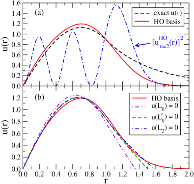
Figure 1: (color online) (a) The exact radial wave function (dashed) for a square well Eq. (3) with depth $V_{0}=4$ (and $\hbar=\mu=R=1$) is compared to the wave function obtained from an HO basis truncated at $N=4$ with $\hbar\Omega=6$ (solid). The spatial extent of the wave function obtained from the HO basis truncation is dictated by the square of HO wave function for the highest radial quantum number (dot-dashed). (b) The wave functions obtained from imposing a Dirichlet boundary condition at $L_{0}$, $L^{\prime}_{0}$ and $L_{2}$ are compared to the wave function in truncated HO basis.

The derivation of the IR correction formula Eq. (1) in Ref. Furnstahl et al. (2012) starts from the observation that a truncated harmonic oscillator (HO) basis effectively acts at low energies to impose a hard-wall boundary condition in coordinate space. In Fig. 1 we can see how this happens for a representative model case, a square well potential Eq. (3) with $s$-wave radial wave functions. In the top panel, the exact ground-state radial wave function (dashed) is compared to the solution in an oscillator basis truncated at $N=4$ determined by diagonalization (solid). The truncated basis cuts off the tail of the exact wave function because the individual basis wave functions have a radial extent that depends on $\hbar\Omega$ (from the Gaussian part) and on the largest power of $r$ (from the polynomial part). The latter is given by $N=2n+l$. With $N=4$ and $l=0$, this means that $n=2$ gives the largest power.

The cutoff will then be determined by the $n=2$ oscillator wave function, $u_{n=2}^{\rm HO}(r)$, whose square (which is the relevant quantity) is also plotted in the top panel (dot-dashed). It is evident that the tail of the wave function in the truncated basis is fixed by this squared wave function. The premise of Ref. Furnstahl et al. (2012) was that this cutoff is well modeled by a hard-wall (Dirichlet) boundary condition at $r=L$. If so, the question remains how best to quantitatively determine $L$ given $N$ and $\hbar\Omega$. Before we present an analytical derivation of this quantity in the next Subsection, we compare empirically $L^{\prime}_{0}$ from Eq. (2) and

$$L_{i}\equiv\sqrt{2(N+3/2+i)}b$$ (7)

with integer $i$, which includes $L_{0}$ as a special case. In the bottom panel of Fig. 1 we show the wave functions for several possible choices for $L$. $L_{0}$ corresponds to choosing the classical turning point (i.e. the half-height point of the tail of $[u^{HO}_{n=2}(r)]^{2}$); it is manifestly too small. Using $L^{\prime}_{0}$, which is the linear extrapolation from the slope at the half-height point, gives an improved estimate. However, choosing $i=2$ (i.e., using $L=L_{2}=\sqrt{2(N+3/2+2)}b$) is found to be the best choice in almost all examples.

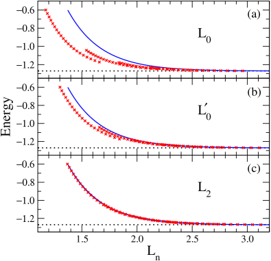
Figure 2: (color online) Ground-state energies versus (a) $L_{0}$, (b) $L^{\prime}_{0}$, and (c) $L_{2}$ for a Gaussian potential well Eq. (5) with $V_{0}=5$ (and $\hbar=\mu=R=1$). The crosses are the energies from HO basis truncation. The energies obtained by numerically solving the Schrödinger equation with a Dirichlet boundary condition at $L$ lie on the solid line. The horizontal dotted lines mark the exact energy, $E_{\infty}=-1.27$.

The most direct illustration of this conclusion comes from the bound-state energies. In the example in Fig. 1, the exact energy (in dimensionless units) is $-1.51$ while the result for the basis truncated at $N=4$ is $-1.33$, which is therefore what we hope to reproduce. With $L_{0}$, the energy is $-0.97$, with $L^{\prime}_{0}$ it is $-1.21$, and with $L_{2}$ it is $-1.29$. While this is only one example of a model problem, we have found that $L_{2}$ always gives a better energy estimate than $L^{\prime}_{0}$ (and $L_{3}$ is almost always worse).

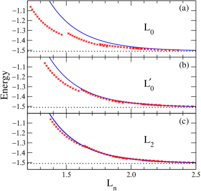
Figure 3: (color online) Ground-state energies versus (a) $L_{0}$, (b) $L^{\prime}_{0}$, and (c) $L_{2}$ for a square well potential well Eq. (3) with $V_{0}=4$ (and $\hbar=\mu=R=1$). The crosses are the energies from HO basis truncation. The energies obtained by numerically solving the Schrödinger equation with a Dirichlet boundary condition at $L$ lie on the solid line. The horizontal dotted lines mark the exact energy, $E_{\infty}=-1.51$.

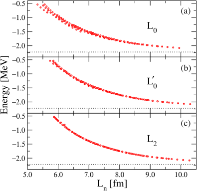
Figure 4: (color online) Ground-state energies versus (a) $L_{0}$, (b) $L^{\prime}_{0}$, and (c) $L_{2}$ for the Entem-Machleidt 500 MeV N³LO potential Entem and Machleidt (2003). The horizontal dotted lines mark the exact energy, $E_{\infty}=-2.2246\,\mbox{MeV}$.

Another signature that demonstrates the suitability of $L_{2}$ is that points from many different $\hbar\Omega$ and $N$ values all lie on the same curve. Figures. 2 and 3 show the energies from a wide range of HO truncations for $L_{0}$, $L^{\prime}_{0}$ and $L_{2}$ for the Gaussian well and the square well potential, respectively. The energies for different $\hbar\Omega$ and $N$ lie on the same smooth and unbroken curve if we use $L_{2}$ but not with the other choices. For $L=L_{0}$ and $L=L^{\prime}_{0}$, one finds that sets of points with different $\hbar\Omega$ but same $N$ fall on smooth, $N$-dependent curves. For the square well, there are small discontinuities visible even for $L=L_{2}$. At the square well radius, the wave function’s second derivative is not smooth, and this is difficult to approximate with a finite set of oscillator functions. This lack of UV convergence is likely the origin of the very small discontinuities. As a further test, we solve the Schrödinger equation with a vanishing Dirichlet boundary condition (solid lines in Figs. 2 and 3) and compare to the energies obtained from the HO truncations (crosses). The finite oscillator basis energies are well approximated by a Dirichlet boundary condition with a mapping from the oscillator $\hbar\Omega$ and $N$ to an equivalent length given by $L_{2}$. Note that for large $N$, the differences between $L_{0}$, $L^{\prime}_{0}$ and $L_{2}$ may be smaller than other uncertainties involved in nuclear calculations, but for practical calculations one will want to use small $N$ results, where these considerations are very relevant.

These results from model calculations are consistent with those from realistic potentials applied to the deuteron. To illustrate this, we use the N³LO 500 MeV potential of Entem and Machleidt Entem and Machleidt (2003). We generate results in an HO basis with $\hbar\Omega$ ranging from $1$ to $100\,\mbox{MeV}$ and $N$ from $4$ to $100$ (in steps of 4 to avoid HO artifacts for the deuteron Bogner et al. (2008)). We then restrict the data to where UV corrections are negligible (see Section IV.3). Figure 4 shows that the criterion of a continuous curve with the smallest spread of points clearly favors $L_{2}$. Similar comments apply to the computation of the radius. Figure 5 shows that the numerical results for the squared radius, when plotted as a function of $L_{2}$ (but not as a function of $L_{0}$), fall on a continuous curve with minimal spread.

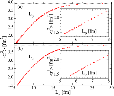
Figure 5: (color online) Deuteron radius squared versus (a) $L_{0}$ and (b) $L_{2}$ for the Entem-Machleidt 500 MeV N³LO potential Entem and Machleidt (2003). The horizontal dotted lines mark the exact radius squared, $r^{2}_{\infty}=3.9006~{}{\rm fm}^{2}$. The insets show a magnification of data at smaller lengths $L_{n}$.

II.2 Analytical derivation of $L_{2}$

Naturally, the squared momentum operator $p^{2}$ is the key for understanding the IR properties of the harmonic oscillator basis. Let us start with the spectrum of $p^{2}$ in the oscillator basis. In a finite basis with energies up to $E=(N+3/2)\hbar\Omega$, the operator $p^{2}$ must be viewed as $p^{2}\Theta(E-p^{2}/(2m)-(m/2)\Omega^{2}r^{2})$, where $\Theta$ denotes the unit step function. Let us compute the number $M(k)$ of $s$-wave states up to a momentum $k$ as a first step. We find

$$M(k) = {\rm Tr}\left[\Theta\left(\hbar^{2}k^{2}-p^{2}\right)\Theta\left(E-{p^{2}\over 2m}-{m\over 2}\Omega^{2}r^{2}\right)\right]$$ (8)

$$\approx {1\over 2\pi\hbar}\int\limits_{-\hbar k}^{\hbar k}\!dp\int\limits_{0}^{\infty}\!dr\,\Theta\left(\hbar^{2}k^{2}-p^{2}\right)$$

$$\hbox{}\times\Theta\left(E-{p^{2}\over 2m}-{m\over 2}\Omega^{2}r^{2}\right)\;.$$

Here, we apply the semiclassical approximation and write the trace as a phase-space integral. We assume $\hbar^{2}k^{2}/(2m)\leq E$, perform the integrations and use $E/(\hbar\Omega)=N+3/2$. This yields

$$M(k) = {bk\over 2\pi}\sqrt{2N+3-b^{2}k^{2}}$$ (9)

$$\hbox{}+{N+3/2\over\pi}\arcsin{bk\over\sqrt{2N+3}}\;,$$

where $b$ is the oscillator length. Figure 6 shows a comparison between the quantum mechanical staircase function and the semiclassical estimate (9) for $N=32$. For sufficiently small values of $kb\ll\sqrt{2N}$, the number of $s$-wave momentum eigenstates grows linearly, and inspection of Eq. (9) shows that the slope at the origin is $L_{0}/\pi$ semiclassically. The linear growth of the number of eigenstates of $p^{2}$ with $k$ clearly demonstrate that — at not too large values of $kb$ — the spectrum of $p^{2}$ in the oscillator basis is indistinguishable from the spectrum of $p^{2}$ in a spherical box. For the determination of the box radius $L$, we note that the lowest eigenvalue of $p^{2}$ is $(\pi/L)^{2}$.

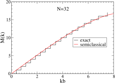
Figure 6: (color online) The staircase function of the $s$ states of the operator $p^{2}$ in a finite oscillator basis with $N=32$ (black) compared to its semiclassical estimate (smooth red curve). $M(k)$ denotes the number of states of the operator $p^{2}$ with eigenvalues $p^{2}\leq\hbar^{2}k^{2}$.

In what follows, we analytically compute the smallest eigenvalue $\kappa^{2}_{\rm min}$ of $p^{2}$ in a finite oscillator basis and will see that $\kappa_{\rm min}=\pi/L_{2}$. In the remainder of this Subsection, we set the oscillator length to one. We focus on $s$-waves and thus consider wave functions that are regular at the origin, i.e. the radial wave functions are identical to the odd wave functions of the one-dimensional harmonic oscillator.

The localized eigenfunction of the operator $p^{2}$ with smallest eigenvalue $\kappa^{2}$ is

$$\psi_{\kappa}(r)=\left\{\begin{array}[]{ll}\sin{\kappa r}\ ,&0\leq r\leq{\pi\over\kappa}\\ 0\ ,&r>{\pi\over\kappa}\end{array}\right.\;.$$ (12)

We employ the $s$-wave oscillator functions

$$\varphi_{2n+1}(r) = (-1)^{n}\sqrt{2n!\over\Gamma(n+3/2)}rL^{1\over 2}_{n}\left(r^{2}\right)e^{-{r^{2}\over 2}}$$

$$= \left(\pi^{1\over 2}2^{2n}(2n+1)!\right)^{-1/2}H_{2n+1}(r)e^{-{r^{2}\over 2}}\;,$$

with energy $E=(2n+3/2)\hbar\Omega$. Here, $L_{n}^{1/2}$ denotes the Laguerre polynomial, and it is convenient to rewrite this function in terms of the Hermite polynomial $H_{n}$. We expand the eigenfunction (12) as

$$\psi_{\kappa}(r)=\sum_{n=0}^{\infty}c_{2n+1}(\kappa)\varphi_{2n+1}(r)\;.$$ (13)

Before we turn to the computation of the expansion coefficients $c_{2n+1}(\kappa)$, we consider the eigenvalue problem for the operator $p^{2}$. We have

$$p^{2}=a^{\dagger}a+{1\over 2}-{1\over 2}\left(a^{2}+\left(a^{\dagger}\right)^{2}\right)\;,$$ (14)

where $a$ and $a^{\dagger}$ denote the annihilation and creation operator for the one-dimensional harmonic oscillator, respectively. The matrix of $p^{2}$ is tridiagonal in the oscillator basis. For the matrix representation, we order the basis states as $(\varphi_{1},\varphi_{3},\varphi_{5},\ldots)$. Thus, the eigenvalue problem $p^{2}-\kappa^{2}=0$ becomes a set of rows of coupled linear equations. In an infinite basis, the eigenvector $(c_{1}(\kappa),c_{3}(\kappa),c_{5}(\kappa),\ldots)$ identically satisfies every row of the eigenvalue problem for any value of $\kappa$. In a finite basis $(\varphi_{1},\varphi_{3},\varphi_{5},\ldots\varphi_{2n+1})$, however, the last row of the eigenvalue problem

$$\left(2n+3/2-\kappa^{2}\right)c_{2n+1}(\kappa)={1\over 2}\sqrt{2n}\sqrt{2n+1}\,c_{2n-1}(\kappa)\;,$$ (15)

can only be fulfilled for certain values of $\kappa$, and this is the quantization condition. To solve this eigenvalue problem we need expressions for the expansion coefficients $c_{2n+1}(\kappa)$ for $n\gg 1$. Those can be derived analytically as follows.

We rewrite the eigenfunction (12) as a Fourier transform

$$\psi_{\kappa}(r)=\sqrt{2\over\pi}\int\limits_{0}^{\infty}dk\tilde{\psi}_{\kappa}(k)\sin kr\;,$$ (16)

and expand the sine function in terms of oscillator functions as

$$\sin kr=\sqrt{\pi\over 2}\sum_{n=0}^{\infty}(-1)^{n}\varphi_{2n+1}(r)\varphi_{2n+1}(k)\;.$$ (17)

Thus, the expansion coefficients in Eq. (13) are given in terms of the Fourier transform $\tilde{\psi}_{\kappa}(k)$ as

$$c_{2n+1}(\kappa)=(-1)^{n}\int\limits_{0}^{\infty}dk\,\tilde{\psi}_{\kappa}(k)\varphi_{2n+1}(k)\;.$$ (18)

So far, all manipulations have been exact. We need an expression for $c_{2n+1}(\kappa)$ for $n\gg 1$ and use the asymptotic expansion

$$\varphi_{2n+1}(k)\approx{(-1)^{n}\sqrt{2}\over\pi^{1/4}}{(2n-1)!!\over\sqrt{(2n)!}}\sin(\sqrt{4n+3}k)\;,$$ (19)

which is valid for $|k|\ll\sqrt{2n}$, see Gradshteyn and Ryzhik (2000). Using this approximation, one finds (making use of Fourier transforms)

$$c_{2n+1}(\kappa) \approx \pi^{1/4}{(2n-1)!!\over\sqrt{(2n)!}}\psi_{\kappa}(\sqrt{4n+3})$$ (20)

$$= \pi^{1/4}{(2n-1)!!\over\sqrt{(2n)!}}\sin(\sqrt{4n+3}\kappa)\;,$$

with $\kappa\leq\pi/\sqrt{4n+3}$ due to Eq. (12).

Let us return to the solution of the quantization condition (15). We make the ansatz

$$\kappa={\pi\over\sqrt{4n+3+2\Delta}}\;,$$ (21)

and must assume that $\Delta>0$. This ansatz is well motivated, since the naive semiclassical estimate $\kappa=\pi/L_{0}$ yields $\Delta=0$. We insert the expansion coefficients (20) into the quantization condition (15) and consider its leading-order approximation for $n\gg 1$ and $n\gg\Delta$. This yields

$$\Delta=2$$ (22)

as the solution. Recalling that a truncation of the basis at $\varphi_{2n+1}$ corresponds to the maximum energy $E=(2n+3/2)\hbar\Omega$, we see that we must identify $N=2n$. Thus, $\kappa_{\rm min}=\pi/L_{2}$ is the lowest momentum (or minimum step of momentum) in a finite oscillator basis with $n\gg 1$ basis states (and not $1/b$ as stated in Ref. Coon et al. (2012)). It is clear from its very definition that $\pi/L_{2}$ is also (a very precise approximation of) the natural infrared cutoff in a finite oscillator basis, and that $L_{2}$ (and not $b$ as stated in Refs. Stetcu et al. (2007a, 2010)) is the radial extent of the oscillator basis and the analogue to the extent of the lattice in lattice computations Lüscher (1986).”

The derivation of our key result $\kappa_{\rm min}=\pi/L_{2}$ is based on the assumption that the number of shells $N$ fulfills $N\gg 1$. Table 1 shows a comparison of numerical results for $\kappa_{\rm min}$ in different model spaces. We see that $\pi/L_{2}$ is a very good approximation already for $N=2$, with a deviation of about 1%.

$N$	$\kappa_{\rm min}$	$\pi/L_{2}$	$\pi/L_{0}$
0	1.2247	1.1874	1.8138
2	0.9586	0.9472	1.1874
4	0.8163	0.8112	0.9472
6	0.7236	0.7207	0.8112
8	0.6568	0.6551	0.7207
10	0.6058	0.6046	0.6551
12	0.5651	0.5642	0.6046
14	0.5316	0.5310	0.5642
16	0.5035	0.5031	0.5310
18	0.4795	0.4791	0.5031
20	0.4585	0.4582	0.4791

Table 1: Comparison between the lowest momentum $\kappa_{\rm min}$, $\pi/L_{2}$, and $\pi/L_{0}$ for model spaces with up to $N$ oscillator quanta.

Note that this approach can be generalized to other localized bases. As the number of basis states is increased, the (numerical) computation of the lowest eigenvalue of the momentum operator $p^{2}$ yields the box size $L$ corresponding to the employed Hilbert space, and results can then be extrapolated according to Eq. (1).

II.3 Scattering phase shifts

The argument for computing scattering phase shifts is as follows: The oscillator basis appears as a spherical box of size $L$. For low momenta we have $L=L_{2}$, but at higher momentum $L$ deviates slightly from $L_{2}$, and can be determined from the eigenvalues of the operator $p^{2}$. Thus, the positive-energy states computed in the oscillator basis can be used to extract phase shifts.

In a fixed harmonic oscillator basis ($N,\hbar\Omega$), the computation of the phase shifts for a given partial wave ${}^{2S+1}l_{J}$ with orbital angular momentum $l$ proceeds as follows: First, one computes the discrete eigenvalues $p_{i}^{2}$ of the operator $p^{2}$ for orbital angular momentum $l$. Second, we need to determine the momentum dependent box size $L_{i}=L(p_{i})$. Assuming that the $i^{\rm th}$ momentum eigenstate is the $i^{\rm th}$ eigenstate of a spherical box, we must determine the $i^{\rm th}$ zero of the spherical Bessel function. Thus $j_{l}(p_{i}L_{i}/\hbar)=0$ determines $L(p_{i})$. We evaluate the smooth function $L(p)$ for arbitrary momentum $p$ by interpolating between the discrete momenta $p_{i}$. Third, we compute the discrete positive energies $E_{i}=\hbar^{2}k_{i}^{2}/(2m)$ of the neutron-proton system in relative coordinates for the partial wave ${}^{2S+1}l_{J}$, and compute the phase shifts from the Dirichlet boundary condition at $r=L$, i.e.

$$\tan\delta_{l}(k_{i})={j_{l}(k_{i}L(\hbar k_{i}))\over\eta_{l}(k_{i}L(\hbar k_{i}))}\;.$$ (23)

Here $\eta_{l}$ is the spherical Neumann function. In practice one repeats this procedure for several values of $\hbar\Omega$ in order to get sufficiently many datapoints that fall onto a smooth curve.

As examples we compute the scattering phase shifts for the ¹S₀ and ³P₁ partial waves in model spaces with $N=32$ and $\hbar\Omega=20,22,\ldots,40$ MeV. Our calculations are based on the Entem-Machleidt 500 MeV chiral EFT N³LO potential Entem and Machleidt (2003). Figures 7 and 8 show the results and compares them to the numerically exact phase shifts. For smaller $N$ than our current choice, the computed phase shifts start to deviate from exact phase shifts at higher energies. However, if one is interested only in low-energy phase shifts and observables such as the scattering length and the effective range, a smaller harmonic oscillator basis is sufficient.

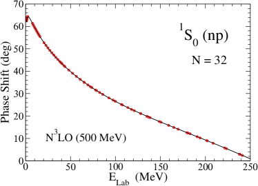
Figure 7: (color online) The ¹S₀ phase shifts (in degrees) of the N³LO chiral interaction (solid line) compared to the phase shifts computed directly in the harmonic oscillator basis (circles).

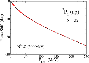
Figure 8: (color online) The ³P₁ phase shifts (in degrees) of the N³LO chiral interaction (solid line) compared to the phase shifts computed directly in the harmonic oscillator basis (circles).

There are other methods to compute scattering phase shifts in the harmonic oscillator basis. Bang et al. Bang et al. (2000) used the method of harmonic oscillator representation of scattering equations (HORSE) for this purpose, and more recent works Luu et al. (2010); Stetcu et al. (2010) computed phase shifts to develop an EFT for nuclear interactions directly in the oscillator basis Stetcu et al. (2007a). References Luu et al. (2010); Stetcu et al. (2010) build on the results by Busch et al. Busch et al. (1998) and their generalization Bhattacharyya and Papenbrock (2006) to finite range corrections, and extract scattering information from the energy shifts of bound states in a harmonic oscillator potential. The resulting EFTs are quite efficient for contact interactions and systems such as ultracold trapped fermions, but nuclear potentials with a finite range require an extrapolation of $\Omega\to 0$ Luu et al. (2010). The approach presented in this Subsection is more direct, as no external oscillator potential is employed. We note that the analysis presented in this Subsection can easily be extended to coupled channels as well.

Finally, we note again that the approach of this Subsection can be utilized in other localized basis sets. All that is required is the diagonalization of the operator $p^{2}$ in the employed basis set, which yields the (momentum dependent) box size.

II.4 Functional dependence of extrapolation

The extrapolation formula (1) with $L=L_{2}$ is theoretically founded. How well can the specific form of this extrapolation be distinguished from other popular empirical choices? To address this question, we test possible functional dependences of the energy correction $\Delta E$ on $L$. The most common extrapolation schemes employ an exponential in $N$ (or equivalently a Gaussian dependence on $L$),

$$E(N)=E_{\infty}+C_{N}e^{-b_{N}N}\;,$$ (24)

where $C_{N}$ and $b_{N}$ are determined separately for each $\hbar\Omega$ (with the option of a constrained fit of a common $E_{\infty}$ for special $\hbar\Omega$ values). Thus, unlike the extrapolation based on $L$, there is no universal variable and no distinction between IR and UV regions in $\hbar\Omega$. However, empirically the form in Eq. (24) seems to work quite well Hagen et al. (2007); Bogner et al. (2008); Forssen et al. (2008); Maris et al. (2009); Roth (2009). Recently, Tolle et al. Tolle et al. (2012) investigated the convergence properties of genuine and smeared contact interactions in an effective theory of trapped bosons and found that the smearing changed a power law dependence of the convergence to an exponential dependence. Here we will consider all three functional dependences on $L$: exponential, Gaussian, and power law.

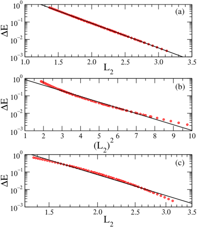
Figure 9: (color online) The IR energy correction $\Delta E_{L}$ versus $L_{2}$ for a Gaussian potential well Eq. (5) with $V_{0}=5$ (and $\hbar=\mu=R=1$) using a wide range of $N$ and $\hbar\Omega$. The energies are fitted with (a) exponential, (b) Gaussian, and (c) power law dependence on $L_{2}$.

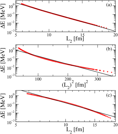
Figure 10: (color online) The IR energy correction $\Delta E_{L}$ versus $L_{2}$ for the deuteron calculated with the chiral EFT potential from Ref. Entem and Machleidt (2003) using a wide range of $N$ and $\hbar\Omega$. The energies are fitted with (a) exponential, (b) Gaussian, and (c) power law dependence on $L_{2}$.

A purely empirical test can be made for our models and the deuteron because we can calculate the exact $E_{\infty}$, plot $\Delta E(L_{2})\equiv E(L_{2})-E_{\infty}$ against $L_{2}$, and then attempt to fit each of the three choices of $\Delta E(L_{2})$. Figure 9 shows the results for a representative model potential (a Gaussian) with moderate depth while Fig. 10 shows the results for the deuteron. The plots are made so that the candidate form would yield a straight line if followed precisely. We see that the exponential form is an excellent fit for the model throughout the range of $L_{2}$ and a reasonable but not perfect fit for the deuteron. For the deuteron, the weak binding is a challenge as it requires very large values of $L_{2}$ for extrapolations. Corrections to weak binding will be derived in Section III. In contrast to the exponential extrapolation, Gaussian and power law fits fail over the full range of $L_{2}$. This is consistent with Tolle et al. Tolle et al. (2012). For limited ranges of $L_{2}$ a Gaussian does provide a reasonable fit (and should give a good extrapolation for $E_{\infty}$ if close enough to convergence), but not globally.

At this stage we have empirically verified the usefulness of the extrapolation (1) in a very controlled setting. This corroborates the study in Ref. Furnstahl et al. (2012) and applications in Refs. Soma et al. (2013); Hergert et al. (2012). The fit result for $k_{\infty}$ has generally been quantitatively consistent with nucleon separation energies (note, however, the case of ⁶He in Ref. Furnstahl et al. (2012)), but the constant $A$ was not identified with physical quantities. The next section will express $A$ in terms of observables for the two-particle system and present corrections to the extrapolation law (1).

III Universal formulas for IR corrections

In this Section we revisit the derivation of Eq. (1) and obtain an expression for the coefficient $A$ in terms of the bound-state asymptotic normalization coefficient (ANC) $\gamma_{\infty}$ and $k_{\infty}$. This is in close analogy to correction formulas for energies calculated with lattice regularization for periodic and hard wall boundary conditions Lüscher (1986); Lee and Pine (2011); Koenig et al. (2012); Pine and Lee (2012). Because $k_{\infty}$ and $\gamma_{\infty}$ are measurable, the result is universal in the sense that it is the same for any potential that reproduces the experimental observables for the bound state. The parameters in Eq. (1) can be fully predicted and tested against precise numerical fits for both our models and the deuteron, which is carried out in Section IV. Corrections to Eq. (1) derived below are found to be quantitatively important for shallow bound states.

III.1 Linear energy approximation

Our first approximation to the IR correction is based on what is known in quantum chemistry as the linear energy method Djajaputra and Cooper (2000). Given a hard-wall boundary condition at $r=L$ beyond the range of the potential, we write the energy compared to that for $L=\infty$ as

$$E_{L}=E_{\infty}+\Delta E_{L}\;.$$ (25)

We seek an estimate for $\Delta E_{L}$, which is assumed to be small, based on an expansion of the wave function in $\Delta E_{L}$. Let $u_{E}(r)$ be a radial solution with regular boundary condition at the origin and energy $E$. For convenience in using standard quantum scattering formalism below, we choose the normalization corresponding to what is called the “regular solution” in Ref. Taylor (2006), which means that $u_{E}(0)=0$ and the slope at the origin is unity for all $E$. We denote the particular solutions $u_{E_{L}}(r)\equiv u_{L}(r)$ and $u_{E_{\infty}}(r)\equiv u_{\infty}(r)$. Then there is a smooth expansion of $u_{E}$ about $E=E_{\infty}$ at fixed $r$, so we approximate Djajaputra and Cooper (2000)

$$u_{L}(r)\approx u_{\infty}(r)+\Delta E_{L}\left.\frac{du_{E}(r)}{dE}\right|_{E_{\infty}}+\mathcal{O}(\Delta E_{L}^{2})\;,$$ (26)

for $r\leq L$. By evaluating Eq. (26) at $r=L$ with the boundary condition $u_{L}(L)=0$, we find

$$\Delta E_{L}\approx-u_{\infty}(L)\left(\left.\frac{du_{E}(L)}{dE}\right|_{E_{\infty}}\right)^{-1}\;,$$ (27)

which is the estimate for the IR correction.

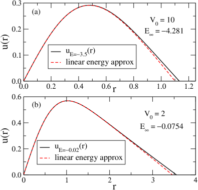
Figure 11: (color online) Testing the linear energy approximation Eq. (26) for (a) deep ($V_{0}=10$) and (b) shallow ($V_{0}=2$) Gaussian potential well Eq. (5) ($\hbar=\mu=R=1$). The solid lines are the exact solutions $u_{L}(r)$ for energies $-3.5$ and $-0.020$, respectively, whose zero crossings determine the corresponding values for $L$.

We can check the accuracy of the linear energy approximation (26) by numerically solving the Schrödinger equation with a specified energy. This determines $L$ as the radius at which the resulting wave function vanishes. Then we compare this wave function for $r\leq L$ to the right side of Eq. (26), with the derivative calculated numerically. Figure 11 shows representative examples for a deep and shallow Gaussian potential. In these examples and other cases, the approximation to the wave function is good, particularly in the interior. The estimates for $\Delta E_{L}$ using the right side of Eq. (27) are within a few to ten percent: 0.68 versus 0.70 and 0.050 versus 0.055 for the two cases.

The good approximation to the wave function suggests that for the calculation of other observables the linear energy approximation will be useful. For observables most sensitive to the long distance (outer) part of the wave function, such as the radius, this has already been shown to be true Furnstahl et al. (2012). But the good approximation to the wave function at small $r$ means that corrections for short-range observables should also be controlled, with the dominant contribution in an extrapolation formula coming from the normalization.

III.2 Complete IR scaling

Next we derive an expression for the derivative in Eq. (27). We assume we have a single partial-wave channel and reserve the generalization to coupled channels (e.g., for a complete treatment of the deuteron) for future work. For general $E<0$, the asymptotic form of the radial wave function for $r$ greater than the range of the potential is (using the notation of Ref. Furnstahl et al. (2012))

$$u_{E}(r)\overset{r\gg R}{\longrightarrow}A_{E}(e^{-k_{E}r}+\alpha_{E}e^{+k_{E}r})\;,$$ (28)

with $u_{\infty}(r)\overset{r\gg R}{\longrightarrow}A_{\infty}e^{-k_{\infty}r}$ for $E=E_{\infty}$. We take the derivative of Eq. (28) with respect to energy, evaluate at $E=E_{\infty}$ using $\alpha_{E_{\infty}}=0$ and $dk_{E}/dE=-\mu/(\hbar^{2}k_{E})$, to find

$$\left.\frac{du_{E}(r)}{dE}\right|_{E_{\infty}} = A_{\infty}\left.\frac{d\alpha_{E}}{dE}\right|_{E_{\infty}}e^{+k_{\infty}r}+A_{\infty}\frac{\mu}{\hbar^{2}}\frac{r}{k_{\infty}}e^{-k_{\infty}r}$$ (29)

$$\hbox{}+\left.\frac{dA_{E}}{dE}\right|_{E_{\infty}}e^{-k_{\infty}r}\;.$$

We now evaluate at $r=L$ and anticipate that the $e^{+k_{\infty}L}$ term dominates:

$$\left.\frac{du_{E}(L)}{dE}\right|_{E_{\infty}}\approx A_{\infty}\left.\frac{d\alpha_{E}}{dE}\right|_{E_{\infty}}e^{+k_{\infty}L}+\mathcal{O}(e^{-k_{\infty}L})\;.$$ (30)

Substituting Eq. (30) into Eq. (27), we obtain

$$\Delta E_{L}\approx-\left[\left.\frac{d\alpha_{E}}{dE}\right|_{E_{\infty}}\right]^{-1}e^{-2k_{\infty}L}+\mathcal{O}(e^{-4k_{\infty}L})\;,$$ (31)

which is in the form of Eq. (1). Note that this result is independent of the normalization of the wave function.

To calculate the derivative explicitly, we turn to scattering theory, following the notation and discussion in Ref. Taylor (2006). In particular, the asymptotic form of the regular scattering wave function $\phi_{l,k}$ for orbital angular momentum $l$ and for positive energy $E\equiv\hbar^{2}k^{2}/2\mu$ is given in terms of the Jost function $\mathfrak{f}_{l}(k)$ Taylor (2006),

$$\phi_{l,k}(r)\longrightarrow\frac{i}{2}[\mathfrak{f}_{l}(k)\hat{h}_{l}^{-}(kr)-\mathfrak{f}_{l}(-k)\hat{h}_{l}^{+}(kr)]\;,$$ (32)

where the $\hat{h}_{l}^{\pm}$ functions (related to Hankel functions) behave asymptotically as

$$\hat{h}_{l}^{\pm}(kr)\overset{r\rightarrow\infty}{\longrightarrow}e^{\pm i(kr-l\pi/2)}\;.$$ (33)

The ratio of the Jost functions appearing in Eq. (32) gives the partial wave $S$-matrix $s_{l}(k)$:

$$s_{l}(k)=\frac{\mathfrak{f}_{l}(-k)}{\mathfrak{f}_{l}(+k)}\;,$$ (34)

which is in turn related to the partial-wave scattering amplitude $f_{l}(k)$ by

$$f_{l}(k)=\frac{s_{l}(k)-1}{2ik}\;.$$ (35)

We will restrict ourselves to $l=0$ for simplicity; the generalization to higher $l$ is straightforward.

To apply Eq. (32) to negative energies, we analytically continue from real to (positive) imaginary $k$. So,

$$\phi_{0,ik_{E}}(r) \overset{r\gg R}{\longrightarrow} \frac{i}{2}\bigl{(}\mathfrak{f}_{0}(ik_{E})e^{k_{E}r}-\mathfrak{f}_{0}(-ik_{E})e^{-k_{E}r}\bigr{)}$$

$$= -\frac{i}{2}\mathfrak{f}_{0}(-ik_{E})\bigl{(}e^{-k_{E}r}-\frac{\mathfrak{f}_{0}(-ik_{E})}{\mathfrak{f}_{0}(ik_{E})}e^{k_{E}r}\bigr{)}\;,$$

where $R$ is the range of the potential. Upon comparing to Eq. (28) we conclude that

$$\alpha_{E}=-\frac{\mathfrak{f}_{0}(ik_{E})}{\mathfrak{f}_{0}(-ik_{E})}=-\frac{1}{s_{0}(ik_{E})}\;.$$ (37)

Note that Eq. (37) is consistent with the bound-state limit of Eq. (28): at a bound state where $E_{\infty}=-\hbar^{2}k_{\infty}^{2}/2\mu$ there is a simple pole in the $S$ matrix, which means $\alpha_{E}=0$ as expected (no exponentially rising piece).

From Ref. Taylor (2006) we learn that the residue as a function of $E$ of the partial wave amplitude $f_{l}(E)$ at the bound-state pole is $(-1)^{l+1}\gamma_{\infty}^{2}\hbar^{2}/2\mu$, where $\gamma_{\infty}$ is the ANC. The ANC is defined by the large-$r$ behavior of the normalized bound-state wave function:

$$u_{\rm norm}(r)\overset{r\gg R}{\longrightarrow}\gamma_{\infty}e^{-k_{\infty}r}\;.$$ (38)

Thus, near the bound-state pole (with $E=\hbar^{2}k^{2}/2\mu$),

$$f_{0}(k)\approx\frac{-\hbar^{2}\gamma_{\infty}^{2}}{2\mu(E-E_{\infty})}=\frac{-\gamma_{\infty}^{2}}{k^{2}+k_{\infty}^{2}}\;.$$ (39)

or, using Eqs. (35) and (37),

$$\alpha_{E}(k)\approx-\frac{k^{2}+k_{\infty}^{2}}{k^{2}+k_{\infty}^{2}-2ik\gamma_{\infty}^{2}}\;.$$ (40)

Now,

$$\left.\frac{d\alpha_{E}}{dE}\right|_{E_{\infty}}=\frac{d\alpha_{E}/dk|_{k=ik_{\infty}}}{dE/dk|_{k=ik_{\infty}}}\;,$$ (41)

so using Eq. (40) we find

$$\left.\frac{d\alpha_{E}}{dk}\right|_{k=ik_{\infty}}=\frac{-i}{\gamma_{\infty}^{2}}\;,$$ (42)

and therefore

$$\left.\frac{d\alpha_{E}}{dE}\right|_{E_{\infty}}=\frac{-\mu}{\hbar^{2}k_{\infty}\gamma_{\infty}^{2}}\;.$$ (43)

Putting it all together, we have

$$\Delta E_{L}=\frac{\hbar^{2}k_{\infty}\gamma_{\infty}^{2}}{\mu}e^{-2k_{\infty}L}+\mathcal{O}(e^{-4k_{\infty}L})\;,$$ (44)

in agreement with Eq. (1), but now we have identified $A=\hbar^{2}k_{\infty}\gamma_{\infty}^{2}/\mu$.

If we apply this correction for a weakly bound state, such that $k_{\infty}$ is small, we may not be justified in neglecting the second term on the right side of Eq. (29). If we keep it instead, then Eq. (30) becomes

$$\left.\frac{du_{E}(L)}{dE}\right|_{E_{\infty}}\approx A_{\infty}e^{+k_{\infty}L}\left(\left.\frac{d\alpha_{E}}{dE}\right|_{E_{\infty}}+\frac{mL}{k_{\infty}}e^{-2k_{\infty}L}\right)\;,$$ (45)

and we have a modified infrared scaling given by

$$(\Delta E_{L})_{\rm mod}=\frac{\hbar^{2}k_{\infty}\gamma_{\infty}^{2}}{\mu}\frac{e^{-2k_{\infty}L}}{(1-\gamma_{\infty}^{2}Le^{-2k_{\infty}L})}\;.$$ (46)

We will test both Eqs. (44) and (46) in Section IV.

III.3 Relation to Lüscher-type formulas

Starting with the seminal work of Lüscher Lüscher (1986), a wide variety of formulas have been derived for the energy shift of bound states in finite-volume lattice calculations. The usual application is to simulations that use periodic boundary conditions in cubic boxes (e.g., see Ref. Koenig et al. (2012)). The recent work by Pine and Lee Lee and Pine (2011); Pine and Lee (2012) extend the derivation to hard-wall boundary conditions using effective field theory for zero-range interactions and the method of images. The result for $\Delta E_{L}$ in a three-dimensional cubic box has a different functional form than found here (the leading exponential is multiplied by $1/L$ with that geometry) and the subleading corrections are parametrically larger.

However, because the HO truncation we consider is in partial waves, the one-dimensional analysis and formula from Ref. Pine and Lee (2012) are applicable (because $k_{\infty}$ and $\gamma_{\infty}$ are asymptotic quantities, the result for zero-range interaction is actually general for short-range interactions). The method of images can be applied in a one-dimensional box of size $2L$ after specializing to a particular partial wave and then extending the space to odd solutions in $r$ from $-\infty$ to $+\infty$. The leading-order finite-volume correction agrees with Eq. (44), and the first omitted term is of the same order. The methods presented in Lee and Pine (2011); Pine and Lee (2012) can be used to extend the present formulas to higher orders and more general cases, including coupled channels.

IV Tests of IR correction formulas

In this Section we test direct fits of Eq. (1), which has three parameters, and the specialized expressions for $\Delta E_{L}$ in Eqs. (44) and (46), which have no free parameters if we take $k_{\infty}$ and $\gamma_{\infty}$ from the exact solutions. Based on the results presented in Sect. II, we use $L_{2}$ in all our further analyses. It is important that we isolate the IR corrections in making these tests. The truncation in the HO basis also introduces an ultraviolet error inversely proportional to the ultraviolet cutoff $\Lambda_{\rm UV}\approx\sqrt{2\mu\hbar\Omega(N+3/2)}$. In the results here we use combinations of $\hbar\Omega$ and $N$ values such that the UV error in each case can be neglected compared to the IR error. (This is verified quantitatively by using a fit ansatz from Ref. Furnstahl et al. (2012) for the UV correction, which is assumed to be independent of the IR correction.)

For each of the model potentials, the radial Schrödinger equation is accurately solved numerically in coordinate space for the energy, which yields $k_{\infty}$, and the wave functions. The asymptotic normalization coefficient $\gamma_{\infty}$ is found by multiplying the wave function by $e^{k_{\infty}r}$ and reading off its asymptotic value. This is illustrated in the inset of Fig. 12, which also shows the onset of the plateau that defines the asymptotic region in $L_{2}$ where we expect our correction formulas to hold. For the deuteron, the Hamiltonian is diagonalized in momentum space to find $k_{\infty}$, and then an extrapolation to the pole is used to find the $s$-wave and $d$-wave ANCs Amado (1979). In the present work we use only the $s$-wave ANC for the deuteron.

IV.1 Universal properties

The derivations in Section III imply that the energy corrections should have the same exponential form and functional dependence on the radius $L$ at which the wave function is zero, independent of the potential and for any bound state (although the relationship between $L$ and the oscillator determined $L_{2}$ is energy dependent). However, there are corrections to Eq. (44) that become increasingly important if $L$ is not sufficiently large. Equation (46) incorporates one such correction but we also have beyond-linear energy corrections and the third term in Eq. (29). Here we make some representative tests of a direct fit of Eq. (1) in comparison to applying Eqs. (44) and (46).

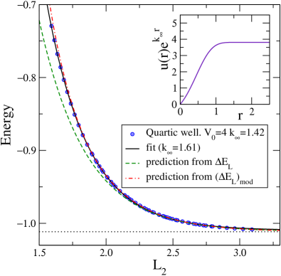
Figure 12: (color online) Energy versus $L_{2}$ for a quartic potential well Eq. (6) for a wide range of $N$ and $\hbar\Omega$ (circles) ($\hbar=\mu=R=1$). The solid line is a fit to Eq. (1) with $A$, $k_{\infty}$ and $E_{\infty}$ as fit parameters while the dashed and dot-dashed lines are predictions from Eqs. (44) and Eq. (46). The horizontal line is the exact energy, $E_{\infty}=-1.0115$. The inset illustrates the calculation of the asymptotic normalization coefficient (ANC) from the (normalized) wave function.

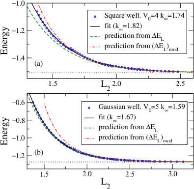
Figure 13: (color online) Energy versus $L_{2}$ for moderate-depth (a) square well Eq. (3) and for (b) Gaussian potential well Eq. (5) ($\hbar=\mu=R=1$) for a wide range of $N$ and $\hbar\Omega$ (circles). The solid line is a fit to Eq. (1) with $A$, $k_{\infty}$ and $E_{\infty}$ as fit parameters while the dashed and dot-dashed lines are predictions from Eqs. (44) and Eq. (46). The horizontal dotted lines are the exact energies; square well: $E_{\infty}=-1.5088$, Gaussian well: $E_{\infty}=-1.2717$

Figure 12 shows results for a quartic potential with a moderate depth. The fit to Eq. (1) is very good over a large range in $L_{2}$ for which the energy changes by 30%, and the prediction for $E_{\infty}$ is accurate to 0.2%. However, the fit value of $k_{\infty}$ is 1.61 compared to the exact value of 1.42. The dashed curve shows the prediction from Eq. (44) using the exact $k_{\infty}$ and $\gamma_{\infty}$. It is evident that the approximation is very good above $L_{2}>2$ but increasingly deviates at smaller $L_{2}$. The modified energy correction from Eq. (46) (dot-dashed curve) matches the energy results at the same level as the fit.

In Fig. 13, examples are shown for square well and Gaussian potentials with a moderate depth. Again we find a good fit to an exponential fall-off in $L_{2}$, but in these cases not only are the energies well predicted (again to better than 0.2%) but the fit values of $k_{\infty}$ are within 5% of the exact results. However, the prediction from Eq. (46) actually degrades the agreement for the Gaussian well compared to the prediction from Eq. (44). Further investigation in these cases reveals that the contributions from the second and third terms in Eq. (29) are of comparable size and opposite sign. Therefore, keeping only one of them is counterproductive.

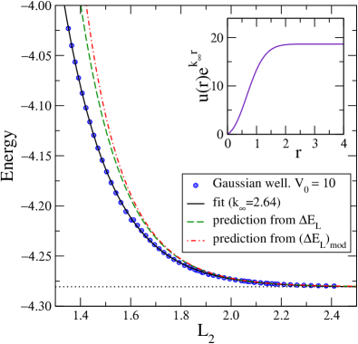
Figure 14: (color online) Energy versus $L_{2}$ for the deeply bound ground state of a Gaussian potential for a wide range of $N$ and $\hbar\Omega$ (circles) ($\hbar=\mu=R=1$). These are compared to the predictions of Eq. (44) (dashed) and Eq. (46) (dot-dashed). The solid line is a fit to Eq. (1) with $A$, $k_{\infty}$ and $E_{\infty}$ as fit parameters. The horizontal dotted line is the exact energy, $E_{\infty}=-4.2806$.

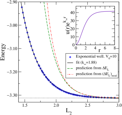
Figure 15: (color online) Energy versus $L_{2}$ for the deeply bound ground state of an exponential potential well for a wide range of $N$ and $\hbar\Omega$ (circles) ($\hbar=\mu=R=1$). These are compared to the predictions of Eq. (44) (dashed) and Eq. (46) (dot-dashed). The solid line is a fit to Eq. (1) with $A$, $k_{\infty}$ and $E_{\infty}$ as fit parameters. The horizontal dotted line is the exact energy, $E_{\infty}=-3.3121$.

For deeply bound states, Eqs. (44) and (46) can fail for a different reason. The error in Eq. (44) is proportional to $e^{-4k_{\infty}L}$, so one might expect that the prediction to become increasingly accurate as the state becomes more bound. However, as seen in Figs. 14 and 15, results for deep Gaussian and exponential potential wells do not match this expectation. In deriving the energy corrections we used the asymptotic form of the wave functions. This is valid only in the region $r\gg R$, where $R$ is the range of the potential. The potentials at the smaller values of $L_{2}$ shown in the figures are not negligible. Indeed, it is evident from the insets in Figs. 14 and 15 that we are not in the asymptotic region for those values of $L$. The lesson is that when applying the IR extrapolation schemes discussed in the present paper we need to make sure that the two conditions for its applicability are fulfilled. First, we need $N$ sufficiently large for $L_{2}$ to be the correct box size (see Table 1). Second we need $L_{2}$ to be the largest length scale in the problem under consideration.

The results in Ref. Furnstahl et al. (2012) and the figures so far are for the ground state of the potential. However, the linear energy approximation and the specific derivations in the last section should also hold for excited states. This is so because the generalization of the results in Subsection II.2 shows that $(j\pi/L_{2})^{2}$ is a very good approximation to the $j^{\rm th}$ eigenvalue of the operator $p^{2}$ for $j\ll N$. In Fig. 16 representative results for excited states from two model potentials are shown. We find the same systematics as with the ground-state results: the exponential fit works very well but the extracted $k_{\infty}$ is only correct at about the 10% level. In assessing the success of Eqs. (44) and (46), we note that these excited states in deep potentials are comparable to the ground states in moderate-depth potentials shown in Fig. 13. The discussion there applies here as well, namely that contributions from the second and third terms in Eq. (29) are of comparable size and opposite sign, so that Eq. (44) alone is a better approximation.

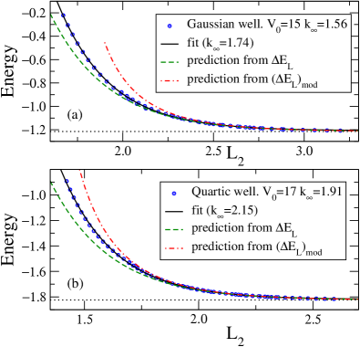
Figure 16: (color online) Energy versus $L_{2}$ for the first excited states of deep (a) Gaussian Eq. (5) and (b) quartic Eq. (6) potential wells for a wide range of $N$ and $\hbar\Omega$ (circles) ($\hbar=\mu=R=1$). The solid line is a fit to Eq. (1) with $A$, $k_{\infty}$ and $E_{\infty}$ as fit parameters while the dashed and dot-dashed lines are predictions from Eqs. (44) and Eq. (46). The horizontal dotted lines are the exact energies for the first excited states; Gaussian well: $E_{\infty}=-1.2147$, quartic well: $E_{\infty}=-1.8236$

In summary, our tests confirm the expectation from Section III that the exponential form of corrections for finite HO basis size is universal for different potentials and also excited states (and also in one dimension, not shown). The leading-order expression Eq. (1) is moderately successful but not quantitative if exact values for $k_{\infty}$ and $\gamma_{\infty}$ are used. This implies that one should not expect to accurately extract $k_{\infty}$ from a fit to Eq. (1). The modified energy correction Eq. (46) is not an improvement for deep potentials because it is not the dominant subleading correction, but we expect it to be the most important correction for shallow bound states (including the deuteron), which we consider next.

IV.2 Shallow bound states

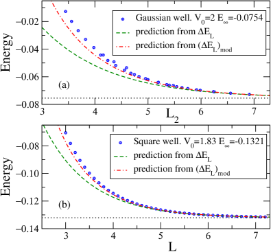
Figure 17: (color online) (a) Ground-state energy versus $L_{2}$ for model Gaussian potential. (b) Energy versus $L$ for the square well. The energies for the square well are from solving the Schrödinger equation exactly with a Dirichlet boundary condition on wave functions at $r=L$. The dashed and dot-dashed lines are predictions from Eqs. (44) and (46). The depths of these model potentials are chosen so that the scaled energies (with $\hbar=\mu=R=1$) are the same as the deuteron binding energy.

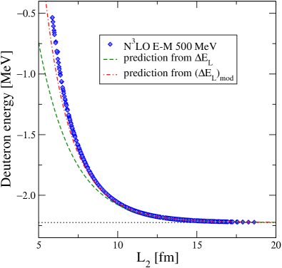
Figure 18: (color online) Deuteron energy versus $L_{2}$ for the potential of Ref. Entem and Machleidt (2003). To eliminate the UV contamination we only keep points for which $\hbar\Omega>49$. The dashed and dot-dashed lines are predictions from Eqs. (44) and (46). The horizontal dotted line is the deuteron binding energy.

The case of weakly bound states is of special interest. Figure 17 (a) shows ground-state energies for many different $N$ and $\hbar\Omega$ versus $L_{2}$ using Gaussian model potentials whose parameters are chosen so that the energies are the same as the deuteron binding energy (scaled to units with $\hbar=1$, $\mu=1$, $R=1$). The prediction Eq. (44) fails to reproduce the data except at the highest values of $L_{2}$. However, when the correction from Eq. (46) is added there is significant improvement. We also note that, contrary to the situation with Figs. 13 and 16, the correction from the third term in Eq. (29) is much smaller and of the same sign as the contribution from the second term included in Eq. (46). This is consistent with the dot-dashed lines falling below the calculated energies at the smallest $L_{2}$ values. In Fig. 17 (b) the same exercise is repeated with a model square well. The energies in this case are obtained by solving the Schrödinger equation exactly with a Dirichlet boundary condition on wave functions at $r=L$. Similar comments as for the model Gaussian potential well also apply here.

In Fig. 18 we show analogous results from the deuteron calculated with the chiral EFT potential of Ref. Entem and Machleidt (2003). As in Fig. 17, the modified IR correction Eq. (46) (evaluated using the $s$-wave ANC) is a significant improvement over Eq. (44), falling slightly below the calculations at the lowest $L_{2}$ values.

IV.3 Effect of SRG evolution

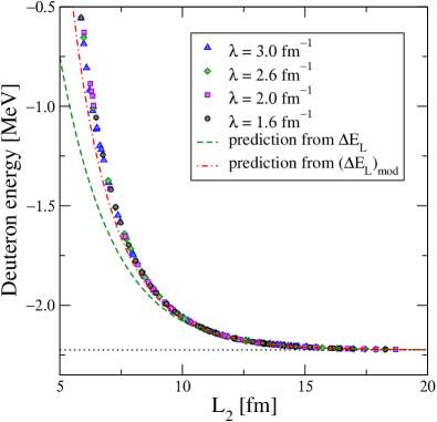
Figure 19: (color online) Deuteron energy versus $L_{2}$ for the potential of Ref. Entem and Machleidt (2003) evolved by the SRG to four different resolutions (specified by $\lambda$). To eliminate the UV contamination we only keep points for which $\hbar\Omega>40$. The dashed and dot-dashed lines are predictions from Eqs. (44) and (46). The horizontal dotted line is the deuteron binding energy.

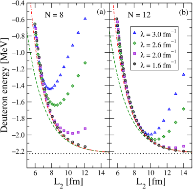
Figure 20: (color online) The same SRG-evolved potentials as in Fig. 19 are used to generate energies, but with $N$ fixed at (a) 8 and (b) 12 and no restriction on $\hbar\Omega$. Thus UV corrections are not negligible everywhere. The dashed and dot-dashed lines are predictions from Eqs. (44) and (46). The horizontal dotted line is the deuteron binding energy.

As a final test of the universal applicability of the correction formulas Eqs. (44) and (46), we consider a sequence of unitarily equivalent potentials for the deuteron. In particular, we use the similarity renormalization group (SRG) Bogner et al. (2010) to evolve the initial Entem-Machleidt potential to four values of the SRG evolution parameter $\lambda$. Because the transformation is exactly unitary (up to very small numerical errors) at the two-body level, the measurable quantities such as phase shifts, bound-state energies, and ANCs are unchanged. As $\lambda$ decreases, the SRG systematically reduces the coupling between high-momentum and low-momentum potential matrix elements, thereby lowering the effective UV cutoff. Thus these potentials are useful tools to assess the role of UV corrections.

We first consider results with $N$ and $\hbar\Omega$ chosen to ensure small UV corrections, as in all prior figures. All the quantities on the RHS of formula Eq. (46) are invariant under SRG evolution. Therefore, if it is an accurate representation of the IR energy corrections from truncating the HO basis, then the $E(L_{2})$ vs $L_{2}$ points for different SRG $\lambda$ should lie on the same curve. Figure 19 shows that this is the case, and the curve is the same as for the unevolved potential in Fig. 18. (Only selected points are plotted for readability.)

Finally, in Fig. 20 we relax the condition that the UV corrections are small compared to IR corrections. In particular, we fix $N$ at 8 and 12 and scan through the full range of $\hbar\Omega$. We observe that with increasing $L_{2}$, each of the curves with a given $\lambda$ eventually deviates from the universal curve, first with $\lambda=3.0\,\text{fm}^{-1}$ and then later with decreasing $\lambda$ or with higher $N$. We can understand this in terms of the behavior of the induced UV cutoff. For fixed $N$, Eq. (7) tells us that increasing $L_{2}$ means increasing $b$ (or decreasing $\hbar\Omega$). But at fixed $N$, $\Lambda_{UV}\propto 1/b$, so the UV cutoff will be decreasing and the corresponding UV energy correction increasing. Thus the curves at fixed $\lambda$ correspond to the curves seen in conventional plots of energy versus $\hbar\Omega$ (e.g., see Ref. Bogner et al. (2008)). The softer potentials (lower $\lambda$) will have lower intrinsic UV cutoffs and therefore they are only affected for larger $L_{2}$. The minima for each $\lambda$ are when IR and UV corrections are roughly equal.

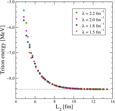
Figure 21: (color online) Triton energy versus $L_{2}$ (here calculated with the deuteron-neutron reduced mass) for the two- and three-nucleon potential in Ref. Jurgenson et al. (2009) unitarily evolved by the SRG to four different resolutions (specified by $\lambda$) with the same binding energy Jurgenson et al. (2009, 2011). Only larger $\hbar\Omega$ points are plotted to minimize the UV contamination. The horizontal dotted line is the exact triton binding energy for this interaction.

V Summary and outlook

In this paper, we revisited the infrared (IR) correction formula derived in Ref. Furnstahl et al. (2012) for a truncated harmonic oscillator (HO) basis expansion, using the simplified case of a two-particle system as a controlled theoretical laboratory. We used simple model potentials and the deuteron calculated with realistic potentials to extend and improve the IR formula. We demonstrated analytically that the spectrum of the squared momentum operator $p^{2}$ in a finite oscillator basis is identical to the one in a spherical box with a hard wall. The minimum eigenvalue of $p^{2}$ is $(\pi\hbar/L_{2})^{2}$, and this identifies $L_{2}$ as the box radius. While these results have been obtained in finite but large oscillator spaces, they also hold in practical applications in much smaller spaces. We showed how errors parametrized in terms of an effective hard-wall radius $L$ from different $N$ and $\hbar\Omega$ combinations all lie on the same curve, but only if the UV error is sufficiently small and, for smaller $N$, only if $L$ is defined as $L_{2}$ (see Eq. (7)). The determination of $L_{2}$ as the box radius also allows us to extract phase shifts from the positive-energy solutions in the oscillator basis.

The fall-off with $L_{2}$ of the IR correction to bound-state energies is found to be an exponential independent of the potential or whether a ground or excited states (or whether we are in one or three dimensions). This conclusion is validated by the derivation and testing of explicit formulas for the energy corrections that depend only on on measurable bound-state properties: the energy and residue of the bound-state pole of the $S$ matrix (or the binding momentum and asymptotic normalization constant).

Tests on larger nuclei have validated the exponential form Eq. (1) with the decay parameter $k_{\infty}$ in the more general case associated with the lowest breakup threshold. Preliminary tests show that $L_{2}$ is also the preferred definition of $L$. An example is shown in Fig. 21, where triton energies for a two- plus three-nucleon potential evolved to four different SRG $\lambda$ (see Refs. Jurgenson et al. (2009, 2011)) lie on the same curve when $L_{2}$ is used. A naive fit to Eq. (44) to the triton assuming a break-up into deuteron plus neutron yields a binding momentum $k_{\infty}\approx 91\,$MeV ($k_{\infty}^{\rm{expt}}=88.13\,$MeV) and ANC $\gamma_{\infty}\approx 3$ fm^-1/2. The ANC is not in agreement with data and previous computations where $\gamma_{\infty}\approx 2$ fm^-1/2 was reported  Huang et al. (2010); Nollett and Wiringa (2011), and suggests that a more sophisticated analysis is necessary for the three-body problem (see also Refs. Kreuzer and Hammer (2011); Polejaeva and Rusetsky (2012); Briceno and Davoudi (2012)). While we expect from general considerations that the parameters of universal curves such as in Fig. 21 are determined by asymptotic (and therefore measurable) quantities, it remains to be investigated whether simple formulas are possible (and whether ANC’s might be approximately extracted from fits).

In most of our investigations here we used our ability to calculate with very large $\hbar\Omega$ and $N$ for two-particle systems to ensure that the effective UV cutoff was large enough to make the UV corrections negligible compared to the IR corrections. However, in realistic calculations we will not (always) have this luxury. The effects of non-negligible UV corrections were shown in Figure 20. By working on the other side of the minimum we can isolate the UV systematics. Analogous studies to those here but on the UV side show that $\Lambda_{UV}$ is an appropriate variable for the energy correction, but the behavior is not universal in the same sense we have identified here. For example, considering different model potentials, ground state vs. excited state, and three dimensions vs. one dimension, we find there are different functional dependencies (see also Ref. Tolle et al. (2012)). While some systematic behavior has been identified for SRG-evolved potentials Furnstahl et al. (2012), further work is needed to go beyond the basic form used to make fits. Work in this direction is in progress.