PARSEC: A Parametrized Simulation Engine for Ultra-High Energy Cosmic Ray Protons

Abstract

We present a new simulation engine for fast generation of ultra-high energy cosmic ray data based on parametrizations of common assumptions of UHECR origin and propagation. Implemented are deflections in unstructured turbulent extragalactic fields, energy losses for protons due to photo–pion production and electron–pair production, as well as effects from the expansion of the universe. Additionally, a simple model to estimate propagation effects from iron nuclei is included. Deflections in the Galactic magnetic field are included using a matrix approach with precalculated lenses generated from backtracked cosmic rays. The PARSEC program is based on object oriented programming paradigms enabling users to extend the implemented models and is steerable with a graphical user interface.

1 Introduction

Recent results of the Pierre Auger Observatory imply that the ultra-high energy cosmic rays (UHECR) are accelerated at extragalactic sources with a distribution following the large scale structure [1, 2]. Nevertheless, the exact origin of these cosmic rays remains so far unknown. UHECR are likely charged particles [2, 3] and thus deflected in the extragalactic and Galactic magnetic field. They can therefore be considered messengers of cosmic accelerators as well as fields they are subjected to while propagating to the Earth. During their propagation from the sources to the Earth UHECR lose energy due to interactions with different photon backgrounds. In the case of protons the dominant processes are photo-pion and electron-pair production, while for nuclei also photo-disintegration has to be accounted for. The composition of UHECR is still under debate [4, 5].

Progress in the understanding of origin and propagation of UHECR is enabled by comparison of measured data with simulated UHECR data. A second field of application for simulated UHECR data is development and benchmarking of observables suited for disentangling specific aspects from the observed data.

The interpretation of cosmic ray data relies on the consideration of models for the:

1. Locations and luminosities of likely sources,

2. Deflections in extragalactic magnetic fields,

3. Composition, and hence energy losses, for the UHECRs, and

4. Deflections in the Galactic magnetic field.

To test these models a fast generation of sufficiently large data samples at every point of the parameter-space is required.

The most obvious approach for a UHECR Monte-Carlo generator allowing detailed simulations of individual physics processes is to follow the trajectories of individual particles from the source to the observer and account for energy losses and deflections during the propagation. This forward-propagation is for example implemented in the CRPropa program [6]. In this approach the, compared to intergalactic distances, small size of the observer makes the generation of large Monte-Carlo data sets, needed for extensive parameter scans, highly challenging. The challenge becomes more and more complex for contributions from distant sources. However, it can be approached by combining forward propagation codes with parametrized simulation software as e.g. presented here; a first attempt of such a combination using CRPropa and PARSEC has been presented in reference [7].

A different approach aiming at UHECR mass production is to backtrack particles starting at the observer and associate them to the objects in the source model. This approach is well understood and documented in the literature (e.g. [8, 9]). However, it requires huge trajectory databases (e.g. [10]) and the trajectories are associated to sources only at the end of the simulation.

To enable UHECR simulations for arbitrary source models with sufficient speed for extensive parameter scans we developed PARSEC as a parametrized simulation engine. PARSEC calculates the probability to observe a particle with energy $E$ from a direction with spherical coordinates $(\phi,\theta$) by summing up the individual contributions of point sources. It uses parameterizations for the energy losses and the effects from deflections in extragalactic magnetic fields to calculate these contributions. Pre-calculated models for the Galactic magnetic field can then be applied in a separate simulation step using matrix techniques. This allows for independent combination of models for extragalactic and Galactic propagation without redundant calculations. From the resulting probability densities, simulated data sets can be generated quickly.

This publication is structured as follows: The implemented models and details of the implementation are presented in section 2. The resulting energy spectra, particle horizons, mean deflections, and exemplary probability density maps are presented together with performance benchmarks in section 3. The conclusions in section 4 are followed by an appendix explaining uncertainties in the generation of the galactic lenses and optional improvements concerning the computing time.

2 Methods

We calculate the probability to observe a particle with energy E from direction $(\phi,\theta)$ in discrete energy bins $E_{i}^{l}\leq E_{i}<E_{i}^{r}$ and discrete directions (pixel) indexed with $j$. For every energy range $i$, the probabilities to observe a particle from all directions $j$ forms a vector $\boldsymbol{p}^{obs}_{i}=(p^{obs}_{i,1},p^{obs}_{i,2},\ldots)^{T}$. The total probability distribution is thus a set of vectors $\mathcal{P}^{obs}=\{\boldsymbol{p}^{obs}_{1},\boldsymbol{p}^{obs}_{2},\ldots\}$ with one vector for every energy range. First, probability vectors $\boldsymbol{p}^{eg}_{i}$ for the expected ‘extragalactic’ distribution including all effects except the Galactic magnetic field are calculated. In a second step this probability vector is transformed by a matrix $\boldsymbol{\mathcal{L}}_{i}$ describing the effects of the galactic magnetic field in energy bin $i$ reading

$$\boldsymbol{\mathcal{L}}_{i}\cdot\boldsymbol{p}^{eg}_{i}=\boldsymbol{p}^{obs}_{i}.$$ (1)

2.1 Extragalactic Propagation

The discrete probability distribution $\boldsymbol{p}^{eg}_{i}$ is calculated by the sum of the contributions of every individual source $S_{k}$ of a source model $\{S_{1}\cdots S_{N}\}$ to every pixel $p_{i,j}$. We separate the contribution of $S_{k}$ to $p_{i,j}$ into three factors:

1. A factor $f^{E}=f^{E}(\gamma,z_{g},B,\Lambda)$ describing the influence of the source spectra with spectral index $\gamma$ and energy loss of the particles. The energy loss depends on the red shift at time of injection of the particle $z_{g}$, and the elongation of the trajectory of the particle by the magnetic field with strength $B$ and coherence length $\Lambda$.

2. A factor $f^{B}=f^{B}(B,\Lambda,D_{k})$ describing the distribution of the flux from a source in distance $D_{k}$ on multiple pixels caused by the magnetic field, and

3. A factor $f^{S}=f^{S}(D_{k},L_{k},B,\Lambda)$ describing the density of particles from source $k$ with luminosity $L_{k}$ after propagation through the extragalactic magnetic field.

With these ingredients the probability to observe a particle with energy $E_{i}$ in pixel $j$ can be written as

$$p_{i,j}=\Gamma_{i}\cdot\sum_{k}f^{E}f^{B}f^{S}$$ (2)

where $\Gamma$ denotes a normalization factor ensuring $\sum_{i,j}p_{i,j}=1$.

2.1.1 Energy Losses

A particle emitted by source $S_{k}$ with the injected energy $E^{inj}$ propagated a distance $c\tau$ within the extragalactic magnetic field model, and is then observed with energy $E_{i}$. Here $c$ is the vacuum speed of light and $\tau$ denotes the propagation time of the particle. The probability to observe the particle therefore depends on the source spectra, the energy loss of the particle and the propagation distance, which is summarized in $f^{E}$. For source spectra following a power law described with spectral index $\gamma$ this corresponds to

$$f^{E}=\frac{1}{1+z_{g}}\left((E_{i}^{inj,r})^{\gamma+1}-(E_{i}^{inj,l})^{\gamma+1}\right)$$ (3)

where the scaling factor $(1+z_{g})^{-1}$ of the universe at the cosmological epoch of particle injection accounts for cosmological time dilation. The range of injection energies $E^{inj,l/r}_{i}$ is calculated with the continuous energy loss approximation by numerically integrating

$$\left(-\frac{1}{E}\frac{dE}{dx}\right)=\frac{1}{L(z,E)}$$ (4)

with the total energy loss length defined as $L(E,z)^{-1}=L_{ad}(z)^{-1}+L_{ph}(E,z)^{-1}$. Here $L_{ad}(z)=c/H(z)$ is the energy loss length for the adiabatic energy loss by the expansion of the universe with Hubble parameter $H(z)=H_{0}\sqrt{\Omega_{m,0}(1+z)^{3}+\Omega_{\Lambda,0}}$ at the cosmological epoch $z$. Here we use for the current matter density $\Omega_{m,0}=0.3$ and the current dark energy density $\Omega_{\Lambda,0}=0.7$ [11].

For the energy loss lengths for interactions in background photon fields $L_{ph}(E,z=0)$ as published in [12, 13] are implemented. Energy loss lengths of alternative models can be easily added. As an extension, we also implemented a simplistic model for the observed UHECR being iron nuclei. For this we also use a continuous energy loss approximation with an attenuation length given by the maximum of the nuclei calculated in reference [14]. Here the iron nuclei do not disintegrate but keep a chargenumber of $Z=26$. The propagation of secondary particles is not included. As the cosmic rays have maximum range and deflections, this model yields a maximum isotropy. From the energy loss length of photon interactions at redshift $z=0$ the energy loss length at $z$ is derived from scaling using

$$L_{ph}(E,z)=(1+z)^{-3}L_{ph}\left((1+z)E,z=0\right)$$ (5)

to account for the increase of the energy and density of the CMB background photons.

2.1.2 Scattering around Sources

The effects of the extragalactic magnetic field are parametrized assuming a turbulent field in which the particles perform a random walk. In a turbulent magnetic field, the flux of a single source $S_{k}$ is distributed over several pixels $p_{i,j}$. If the particles perform a random walk, the distribution of the angles $\alpha_{j,k}$ between the direction of source $S_{k}$ and the center of pixel $p_{i,j}$ follows a Fisher distribution [15], which can be regarded as normal distribution on a sphere. The second factor $f^{B}$ of eq. 2 thus reads

$$f^{B}(\alpha_{j,k},\kappa)=\frac{\kappa}{4\pi\sinh{(\kappa)}}e^{(\kappa\cdot\cos{\alpha_{j,k})}}$$ (6)

with the concentration parameter $\kappa$.

The concentration parameter $\kappa$ is related to the root mean square (rms) $\sigma$ of the deflection for small angles by $\kappa=1/\sigma^{2}$ [16]. For small angles the root mean square of the deflection of UHECR with charge $Z$ in units of the electron charge $e$ in turbulent fields with $D_{k}\gg\Lambda$ can be parametrized [17] as

$$\sigma=\frac{37.5^{\circ}}{\sqrt{3}}\sqrt{\frac{D_{k}}{\Lambda}}\left(\frac{\Lambda}{\mathrm{Mpc}}\right)\left(\frac{B}{\mathrm{nG}}\right)\left(\frac{Z}{e}\right)\left(\frac{E}{\mathrm{EeV}}\right)^{-1}.$$ (7)

Here $D_{k}$ is the current proper distance of $S_{k}$ to the observer, $B$ is the strength of the magnetic field, and

$$\Lambda=\frac{\pi}{B^{2}}\int_{0}^{\infty}\frac{dk}{k}B^{2}(k)$$ (8)

the correlation length of the magnetic field [18, 17]. For a Kolmogorov turbulent field with spectral index $n$ and minimum, respectively maximum, correlation length $L_{\min,\max}$ it is

$$\Lambda=\frac{1}{2}L_{\max}\frac{n-1}{n}\frac{{(1-L_{\min}/L_{\max})}^{n}}{1-{(L_{\min}/L_{\max})}^{n-1}}.$$ (9)

This parametrization for the rms of the deflection angle does not include energy losses. To derive a first order approximation including energy losses, we first differentiate eq. 7 with respect to the source distance. Using $x$ as variable for the source distance this reads

$$\frac{d\sigma}{dx}=\frac{37.5^{\circ}}{\sqrt{3}}\sqrt{\frac{\Lambda}{x}}\frac{B}{E(x)}\left(1-\frac{x}{E}\frac{dE}{dx}\right).$$ (10)

Assuming $(dE/dx)\cdot(x/E)$ being small for the ultra-high energies considered here the second term of eq. 10 can be neglected. Integrating eq. 10 to the source distance

$$\sigma=\frac{37.5^{\circ}}{\sqrt{3}}\sqrt{\frac{\Lambda}{x}}B\int_{0}^{D_{k}}\frac{1}{E(x)}dx$$ (11)

then yields the rms of the deflection for particles from source $S_{k}$.

2.1.3 Elongation of Propagation Time

Due to deflection in magnetic fields the length of the trajectory of the particles $c\tau=D_{k}+r$ from sources in distance $D_{k}$ is elongated by an extra distance $r$. Neglecting energy losses, the additional propagation distance $r$ originating from small deflections in the extragalactic magnetic field can be written as

$$r=116\mathrm{\leavevmode\nobreak\ kpc}\left(\frac{B}{\mathrm{nG}}\right)^{2}\left(\frac{Z}{e}\right)^{2}\left(\frac{D_{k}}{\mathrm{Mpc}}\right)^{2}\left(\frac{E}{\mathrm{EeV}}\right)^{-2}\left(\frac{\Lambda}{\mathrm{Mpc}}\right)$$ (12)

with definitions as in eq. 7 [18]. To account for energy losses in the extended propagation length we write eq. 12 for infinitely small $dx$

$$dr\propto\left(\frac{2xB^{2}\Lambda Z^{2}}{E^{2}}dx-\frac{2B^{2}x^{2}\Lambda Z^{2}}{E^{3}}\frac{dE}{dx}dx\right)$$ (13)

with $0<x\leq D_{k}$. The proportionality constant is given by eq. 12. Assuming again $(dE/dx)\cdot(x/E)$ to be small, the second term of eq. 13 can be neglected. The result can be written as a Riemann sum

$$r\propto\sum_{i}^{N}\frac{B^{2}\Lambda Z^{2}}{E\left(x_{i}+\frac{(x_{i}-x_{i-1})}{2}\right)^{2}}(x_{i}^{2}-x_{i-1}^{2})$$ (14)

with $x_{N}=D_{k}$.

2.1.4 Increase of Particle Density

The factor $f_{S}$ accounts for the relative individual luminosity $L_{k}$ of source $S_{k}$ and the density of particles at the position of the observer in current proper distance $D_{k}$. If the particles propagate on a straight line, the flux from a source is distributed on a sphere with radius of the current proper distance $D_{k}$ of the source resulting in $f_{S}=L_{k}/D_{k}^{2}$.

Nevertheless, in the presence of magnetic fields the density of UHECR is higher compared with linear propagation. In some distance to the source all information about the origin of the UHECR is lost, and instead of a directed random walk the density is described according to a undirected random walk. To model this transition we simulated the trajectories of individual UHECR from one source in a turbulent magnetic field using the CRPropa software [19]. Using $g=\frac{B}{E}\sqrt{\Lambda}$ the density of UHECR in distance $D_{k}$ can be approximatly described by

$$f_{S}=\frac{L_{k}}{D_{k}^{2}}\left((1+p_{1}\cdot g^{2}\cdot D_{k})(1-T)+T\cdot p_{2}\cdot g\cdot e^{-\frac{1}{2}\left(\frac{D_{k}}{x_{1}}\cdot g-1\right)^{2}}\right)$$ (15)

with

$$T=\frac{1}{1+\left(\frac{D_{k}\cdot g}{x_{t}}\right)^{-s}}.$$ (16)

and parameters as given in table 1.

Table 1: Results of the fit of eq. 15 to UHECR densities in forward simulations.

Parameter	Val	ue	Unit
$p_{1}$	0	.1	$\mathrm{nG}^{-2}\,\mathrm{EeV}^{2}\,\mathrm{Mpc}^{-3/2}$
$s$	5		—
$x_{t}$	70		$\mathrm{nG\leavevmode\nobreak\ EeV}^{-1}\,\mathrm{Mpc}^{3/2}$
$p_{2}$	9		$\mathrm{nG}^{-1}\,\mathrm{EeV}\,\mathrm{Mpc}^{-1/2}$
$x_{1}$	140		$\mathrm{nG}\,\mathrm{EeV}^{-1}\,\mathrm{Mpc}^{3/2}$:

For $0.1\,\mathrm{nG\leavevmode\nobreak\ EeV}^{-1}\,\mathrm{Mpc}^{1/2}<g<2.5\,\mathrm{nG\leavevmode\nobreak\ EeV}^{-1}\,\mathrm{Mpc}^{1/2}$ the deviation of eq. 15 from the simulated values is typically below 20%. For a homogeneous distribution of sources, the resulting observed spectrum agrees also within 20% with the universal spectrum [20].

2.2 Galactic Magnetic Field

To model particle propagation in the Galactic magnetic field we neglect energy losses during the relatively short Galactic propagation. As there is no random process in this model, the trajectories of all cosmic rays with energy $E_{i}$ traversing the Galaxy are completely defined by the point of entry into the Galaxy $\boldsymbol{C}$ and their direction $(\phi,\theta)$. The effects of the Galactic magnetic field can thus be addressed as magnetic lensing, i.e. a mapping of every point of the phase space $(\boldsymbol{C},\theta,\phi)_{eg}$ outside the Galaxy, i.e. where the effect of the Galactic magnetic field can be neglected, to a point $(\boldsymbol{D},\theta,\phi)_{obs}$ within the Galaxy [21, 22].

We assume that the observed spatial density of cosmic rays does not depend strongly on the position of the observer so that Earth can be safely modelled as point and only the directions from which a particle are observed at the position of the Earth are relevant. We index the discrete observed directions (pixel) with $m$. A particle with energy $E_{i}$ entering the galaxy at a point $\boldsymbol{C}$ on the surface of the galaxy at a discrete direction denoted with index $n$ is thus always observed at Earth at direction $m$.

The sources considered here are generally in a large distance compared to the size of the galaxy, which reduces the galaxy to a point in view of the source. We assume that the spatial density of cosmic rays from one source on the edge of the Galaxy, i.e. the sphere which encloses the volume for which the Galactic magnetic field is considered, is governed by geometry and not by effects from deflection in the extragalactic magnetic field. The directions of entry $n$ for particles with energies $E_{i}$ can therefore be averaged over all points of entry $\boldsymbol{C}$. Thus, and due to the limited number of pixels, a particle with energy $E_{i}$ entering the galaxy from direction $n$ can be deflected into several observed directions $m$.

The probability of observing a particle on Earth from direction $m$ which entered the galaxy from direction $n$ is $l_{m,n}$. The $l_{m,n}$ form a matrix $\boldsymbol{\mathcal{L}}_{i}$ which represents the galactic lens for energy $E_{i}$. The model for the Galactic magnetic field is completely described by a set of matrices $\{\boldsymbol{\mathcal{L}}_{1}\cdots\boldsymbol{\mathcal{L}}_{N}\}$ with the energy index $i=1\ldots N$.

The individual matrices $\boldsymbol{\mathcal{L}}_{i}$ can be generated by backtracking cosmic rays with isotropic starting directions from the earth with the following technique. The starting directions of backtracked particles are binned in $N$ pixels indexed by $m$. The directions in which the cosmic rays leave the galaxy are binned into $N$ pixels indexed by $n$. Counting all trajectories leads to a matrix $\boldsymbol{\mathcal{\tilde{L}}}_{i}$ with elements $\tilde{l}_{m,n}$. For three directions and nine backtracked particles the procedure is illustrated in figure 1. We normalize $\boldsymbol{\mathcal{\tilde{L}}}_{i}$ by the maximum of unity norms $\|\boldsymbol{\mathcal{\tilde{L}}}_{i}\|_{1}$ of all lenses reading

$$\boldsymbol{\mathcal{L}}_{i}=\frac{1}{\max{\|\boldsymbol{\mathcal{\tilde{L}}}_{i}\|_{1}}}\boldsymbol{\mathcal{\tilde{L}}}_{i}.$$ (17)

Each element $l_{m,n}$ of $\boldsymbol{\mathcal{L}}_{i}$ is the probability that a particle entering the galaxy in pixel $n$ is observed in direction $m$.

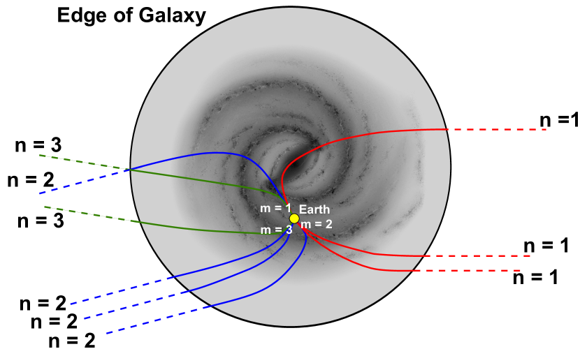
Figure 1: Sketch of the creation of a galactic lens from backtracking data. Cosmic rays are emitted from earth in three directions indexed with $m$. The directions in which the rays leave the galaxy are indexed with $n$.

As a consequence of Liouville’s theorem, that the phase space along trajectories that satisfy the Hamiltonian equations is constant, an isotropic distribution of cosmic rays outside the galaxy is observed as an isotropic distribution at any point of the galaxy [23, 24, 22]. This important property of the Galactic magnetic field is correctly modeled by this technique, if the directions $m$ are uniformly sampled in the backtracking, respectively the unity norm $\|.\|_{1}$ of all row vectors $\boldsymbol{l}_{m}$ are identical.

In general the Galactic magnetic field modifies the energy spectrum of cosmic rays depending on the positions of the sources $S_{k}$ as the flux from individual regions in the sky is suppressed or enhanced [22]. While the relative deformation of the energy spectrum is accounted for in the normalization procedure described above, no information about a suppression of the total flux by the Galactic magnetic field is obtained by the generation of the galactic lenses from backtracking.

Galactic lenses, generated from backtracking Monte-Carlo data in the described way, introduce an uncertainty in the observed probability distribution. This uncertainty is discussed in A.1.

2.3 Technical Realization

PARSEC is implemented as C++ code with a Python interface. It is based on the Physics Extension Library (PXL) [25]. PXL is a collection of C++ libraries with a Python interface providing classes and templates for experiment independent high-level physics analysis. The usage of the PXL libraries facilitates modular object-oriented programming and allows graphical steering of the simulation components using the VISPA program [26].

The individual simulation steps are implemented as separate PXL modules which can be individually connected and configured to a simulation chain using the graphical user interface (GUI) of VISPA. A realization of a UHECR scenario is represented by a data container, which is consecutively processed by the following modules.

Source Model

Sources of UHECR are represented as individual objects. They are added to the realization with user-defined coordinates in a Python or C++ module. An exemplary module for isotropic source distributions is included in PARSEC. Modules generating sources e.g. from astronomical catalogues can be created by users.

Extragalactic Field Model

From the sources in the simulation the probability vectors for extragalactic propagation are calculated for a user-defined discretization of the energies and directions. The calculation is separated into C++ classes for the propagation and the energy loss, each based on an abstract interface. The abstract interfaces are implemented as subtypes for the random-walk propagation in turbulent fields, respectively the described energy loss for proton and iron UHECR. This polymorphic design enables users to modify and extend the individual components independently.

Galactic Field Model

For an angular resolution of the discretization better than $\approx 1^{\circ}$ matrices of about $50000\times 50000$ elements are needed. However, as in typical Galactic magnetic field models particles from most directions are not distributed over the whole sky, the matrices $\boldsymbol{\mathcal{L}}_{i}$ are only sparsely populated. The lenses for the Galactic field are consequently implemented using a common linear algebra library which features sparse matrices [27]. This enables calculation of eq. 1 with reasonable consumption of resources. PARSEC includes tools for generation of the lenses from backtracking data from the CRT [9] and CRPropa [19] programs.

The galactic lenses are independent of the PARSEC module for the extragalactic propagation and can be used to calculate the deflection of individual cosmic rays. Spline interpolation and numeric integration routines used in the program are taken from the GNU Scientific Library [28].

3 Results

3.1 Energy spectrum

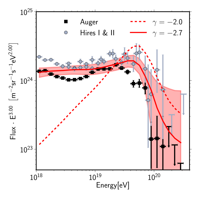
Figure 2: Energy spectra of UHECR generated by PARSEC and observed spectra reported by the Pierre Auger Observatory [29] and the HiRes experiment [30]. The simulation results are obtained from sources with spectral indices $\gamma=-2.7$ and $\gamma=-2.0$ in an extragalactic magnetic field with $B=1$ nG and $\Lambda=1$ Mpc. The shaded regions indicate the spread in the simulated realizations.

The energy spectrum of cosmic rays is a key distribution for comparisons of models with observations. From PARSEC simulations the energy spectra $dN/dE(E_{i})$ are calculated using $dN/dE(E_{i})=\hat{L}\cdot\|\boldsymbol{p}_{i}\|_{1}$ with normalization factor $\hat{L}=L_{0}/\sum_{i}^{N}L_{i}$ where the luminosity scale $L_{0}$ fitted to data or set by a source model.

In Figure 2 energy spectra obtained with the PARSEC program are compared with the observed energy spectra of the Pierre Auger Observatory [29] and HiRes experiment [30]. The spread of the energy spectra of 50 realizations with different source positions and the mean energy spectrum are shown for two different spectral indices $\gamma$ of the injection spectra. The simulated spectra were generated using isotropically distributed sources with a density of $10^{-5}$ Mpc^-3 and an extragalactic field of strength $B=1$ nG with correlation length $\Lambda=1$ Mpc. The probability maps $\boldsymbol{p}_{i}$ have been calculated for 100 log-linear spaced energies $E_{i}$ from $10^{18.5}$ eV to $10^{20.5}$ eV in the simulation. The normalization factor $\hat{L}$ has been fitted to match the result from the Pierre Auger Collaboration at an energy of 22 EeV.

3.2 Particle horizons

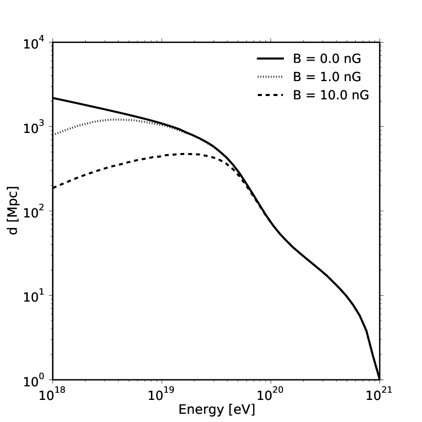
Figure 3: Horizon $d$ for protons with observed energy $E$. The curves show $d$ for several strengths of a turbulent magnetic field $B$ with correlation length $\Lambda=1$ Mpc.

From the maximum injection energy $E_{max}$ and the model of the energy loss a particle horizon can be derived which corresponds to the maximum linear distance a particle can originate from. Following eq. 14 this horizon depends on the extragalactic magnetic field model and the observed particle energy. In Figure 3 the horizon for different field strengths is shown as a function of the energy for sources with a maximum injection energy of $E_{max}=1000$ EeV.

In case of a non-zero extragalactic magnetic field, the horizon is reduced as the trajectories are elongated. The effect is visible below $20$ EeV for a $1$ nG field and at higher energies for stronger fields. Without scaling the energy losses with red-shift $z$, the horizon is not reduced for lower energetic particles, as the energy loss only depends on the particles energy and not the time. The energy thus monotonically increases with the linear distance.

For an energy of 100 EeV the distance from within 90% of the UHECR flux originates from is calculated to $d_{90}$ = 45 Mpc in case of zero magnetic field and a spectral index of the sources $\gamma=2.0$. This is $\approx 30\%$ lower than the result obtained from simulations with CRPropa [6] and a known feature of the continuous energy loss approximation [31].

3.3 Mean Deflection in Magnetic Fields

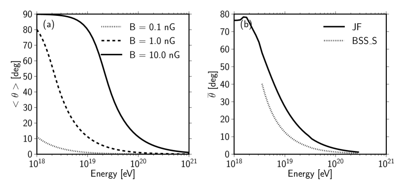
Figure 4: Mean deflection of cosmic ray protons in (a) turbulent extragalactic fields and (b) BSS_S and JF Galactic magnetic field model.

The expectation value for an angle $\theta$ following a Fisher distribution with concentration parameter $\kappa$ is calculated as

$$\langle\theta\rangle=\frac{\pi}{2\sinh{\kappa}}\cdot(I_{0}(\kappa)-e^{-\kappa})$$ (18)

with $I_{0}$ representing the modified Bessel function of order $0$. From this the mean deflection in the extragalactic field can be calculated for the parameters of the magnetic field and source model using eq. 7.

In Figure 4 a) the mean deflection of protons from a source at 10 Mpc distance in extragalactic magnetic fields with three different strengths and a coherence length $\Lambda=1$ Mpc are shown as a function of the energy. A mean deflection of $90^{\circ}$ corresponds to an isotropic arrival distribution of the UHECR.

The mean deflections $\bar{\Theta}$ in the Galactic magnetic field can be directly calculated from the lens $\boldsymbol{\mathcal{L}}_{i}$ as

$$\bar{\Theta}=\frac{1}{\sum_{m,n}l_{m,n}}\sum_{m,n}l_{m,n}\arccos{\left(\boldsymbol{e}_{m}\cdot\boldsymbol{e}_{n}\right)}$$ (19)

with $\boldsymbol{e}_{n},\boldsymbol{e_{m}}$ being the unit vector in the direction of pixel $m$, respectively $n$. In general the mean deflection in the Galactic magnetic field depends on the source configuration due to the suppression of individual regions by the galactic lens. In Figure 4 b) the mean deflection from lenses for the JF model [32] and the BSS_S model [33, 21] of the Galactic magnetic field are displayed. For the BSS_S model a field normalization of $B_{0}=0.48\leavevmode\nobreak\ \mu$G and scale heights of $z_{1}=0.95$ kpc and $z_{2}=4.0$ kpc were chosen.

3.4 Exemplary Probability Distributions

To demonstrate the capabilities of PARSEC we generated an exemplary result with source positions taken from the 12th edition of the catalogue of quasars and active galactic nuclei (AGN) by Véron-Cetty and Véron [34]. Every AGN of the catalogue up to a distance of 1000 Mpc has been considered. For the extragalactic field we chose a field strength $B=3$ nG and a correlation length of $\Lambda=1$ Mpc. The resulting probability maps from the extragalactic propagation $\boldsymbol{p}_{eg}^{i}$ are shown in the top row of Figure 5 for the two different energies $E_{1}=10$ EeV (Fig. 5 a) and $E_{2}=30$ EeV (Fig. 5 b).

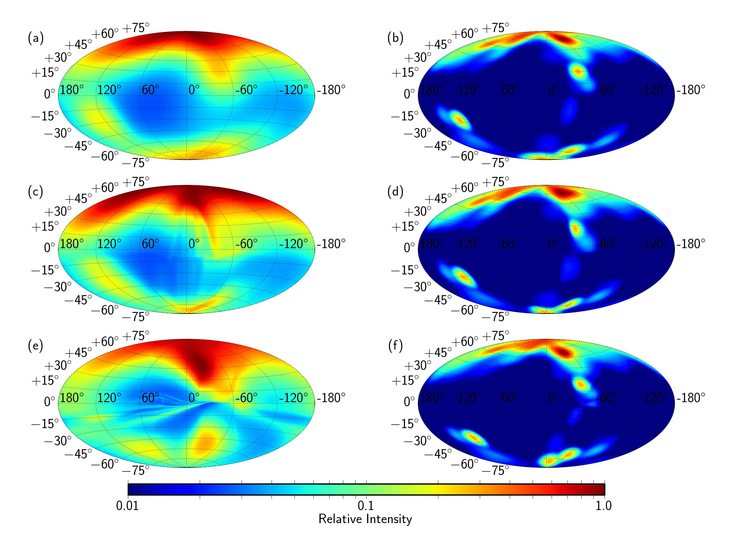
Figure 5: Hammer projected probability density maps for cosmic ray protons with an observed energy of $E=10$ EeV (left column) and $E=30$ EeV (right column) in galactic coordinates. Red indicates higher, blue lower probability on an arbitrary scale. From top to bottom the panels show: (a,b) Probability density before applying the galactic lens, (c,d) probability density after application of the galactic lens of a BSS_S model, and (e,f) probability density after application of the galactic lens for the JF2012 model.

The second row of Figure 5 (c,d) displays the same probability maps after application of the galactic lenses for a BSS_S model of the Galactic magnetic field with a normalization of $B_{0}=0.48\leavevmode\nobreak\ \mu$G and scale heights of $z_{1}=0.95$ kpc and $z_{2}=4.0$ kpc. The lenses have been created by backtracking $10^{6}$ protons with the CRT program [9] for 100 log-linear spaced mono-energetic simulations from $10^{18.5}$ eV to $10^{20.5}$ eV. The lenses and probability vectors have been discretized into 49,152 equal area pixels following the scheme implemented in the HEALpix software [35]. The third row of Figure 5 (e,f) shows the probability maps of (a,b) after application of a lens for the JF model [32] of the Galactic magnetic field.

3.5 Performance

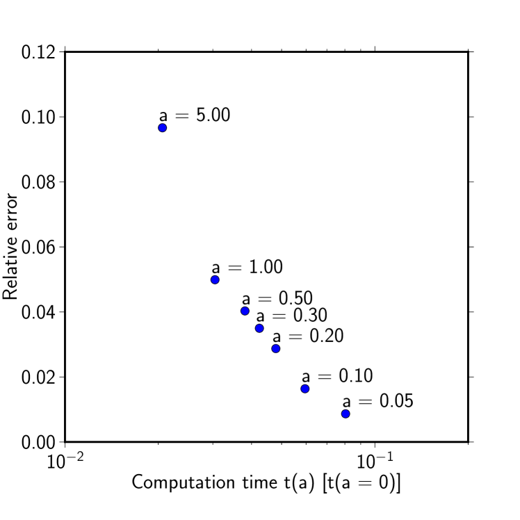
Figure 6: Computation time for the exemplary scenario and resulting error $\epsilon$ for different choices of the cut-off parameter $a$. Times are given in units of the time needed for the full calculation.

The exemplary simulation was performed in 6,690 sec using a single core of a Lenovo Thinkpad T400 notebook with 4 GB RAM and an Intel Core 2 Duo P8600 2.4 GHz CPU. The notebook has been benchmarked with a SPECfp_base2006 rate of 12.2 and SPECint_base2006 rate of 15.1 [36]. Peak memory usage of the program was 0.5 GB. The size of the BSS_S magnetic lens on disk is 262 MB.

The performance can be improved by approximating the individual contribution from distant sources as an isotropic component. This approximation introduces an error $\epsilon$ to the extragalactic probability vector $\boldsymbol{p}_{eg}^{i}$. An example realization with isotropic source distribution with $10^{-4}$ sources per Mpc³ up to 1000 Mpc is used to demonstrate the effect. In Figure 6 the resulting error $\epsilon=\|\boldsymbol{p}_{unbiased}-\boldsymbol{p}_{biased}\|_{1}$ is displayed as a function of the computation time for various values of the cut-off parameter $a$ (see A.2). Here $a$ represents a measure of the strength of the anisotropic signal contribution not considered in the calculation. By this method the computation time can be reduced by an order of of magnitude for $a=0.05$, which introduces an uncertainty less than 1%.

4 Conclusions

We have presented a parametrized Monte-Carlo generator for fast creation of simulated UHECR datasets. The code includes effects of proton propagation through extragalactic and Galactic magnetic field models as well as energy losses during propagation. Also implemented is an extension to a simple model of iron propagation. Arbitrary source models can be easily tested with the code. The generation of datasets is sufficiently fast to enable extensive parameter scans of the models. The modular design of PARSEC combined with the graphical steering is suited for user extensions of the code and implementation of user defined models. The source code of PARSEC as well as exemplary magnetic lenses are available under a GNU General Public License from http://www.physik.rwth-aachen.de/parsec.

Appendix A Appendix

A.1 Uncertainties of Galactic Lenses

From two realizations of the same model for the galactic magnetic field an upper limit of the introduced error can be derived as follows. For eq. 1 it is $\|\boldsymbol{p}_{obs.}\|_{1}\leq 1$ as individual regions of the sky are suppressed. However, from $\boldsymbol{\mathcal{L}}\in\mathbb{R}^{N\times N}$ with $l_{m,n}$ we can generate

$$\boldsymbol{\mathcal{\hat{L}}}=\left(\begin{array}[]{ccc}l_{1,1}&\cdots&l_{1,N}\\ \vdots&\ddots&\vdots\\ l_{N,1}&\cdots&l_{N,N}\\ s_{1}&\cdots&s_{N}\\ \end{array}\right)$$ (20)

with $\boldsymbol{\mathcal{\hat{L}}}\in\mathbb{R}^{N+1\times N}$ and $s_{n}=1-\|\boldsymbol{l}_{n}\|_{1}$ such that $\boldsymbol{\mathcal{\hat{L}}}\cdot\boldsymbol{p}_{eg}=\boldsymbol{\hat{p}}_{o}$ with $\boldsymbol{\hat{p}}_{o}\in\mathbb{R}^{N+1}$ and $\boldsymbol{\hat{p}}_{o}^{T}=(p_{1},\cdots p_{N},s)$. $s_{n}$ represents the suppression the UHECR flux from the extragalactic direction $n$ and $s=\sum s_{n}$ the total suppression of $\boldsymbol{p}_{eg}$ by $\boldsymbol{\mathcal{L}}$. By this definitions it is $\|\boldsymbol{\hat{p}}_{o}\|_{1}=1$.

Let $\boldsymbol{\mathcal{\hat{L}}}_{1}$ be a realization of the ‘true’ lens $\boldsymbol{\mathcal{\hat{L}}}$, then application of $\boldsymbol{\mathcal{\hat{L}}}_{1}$ in eq. 1 introduces an uncertainty $\boldsymbol{\hat{\delta p}}$

$$\boldsymbol{\mathcal{\hat{L}}}_{1}\cdot\boldsymbol{p}_{eg}=\boldsymbol{\hat{p}}_{o}+\boldsymbol{\hat{\delta p}}$$ (21)

which depends on the extragalactic probability density $\boldsymbol{p}_{eg}$, or the individual configurations of the source and extragalactic propagation models, respectively.

If $\boldsymbol{p}_{eg}$ is known, the uncertainty can be calculated, as we can approximate the true lens $\boldsymbol{\mathcal{\hat{L}}}$ by the mean of individual realizations. In the following calculations only two realizations $\boldsymbol{\mathcal{\hat{L}}}_{1}$ and $\boldsymbol{\mathcal{\hat{L}}}_{2}$ of $\boldsymbol{\mathcal{\hat{L}}}$ are used in order of clarity.

For two realizations the true lens can be approximated as $\boldsymbol{\mathcal{\hat{L}}}=\frac{1}{2}(\boldsymbol{\mathcal{\hat{L}}}_{1}+\boldsymbol{\mathcal{\hat{L}}}_{2})$. Using this we substitute $\boldsymbol{\mathcal{\hat{L}}}_{1}$ in eq. 21 which yields

$$\frac{1}{2}\boldsymbol{\mathcal{\delta\hat{L}}}\cdot\boldsymbol{p}_{eg}=\boldsymbol{\hat{\delta p}}$$ (22)

with $\boldsymbol{\mathcal{\delta\hat{L}}}=\boldsymbol{\mathcal{\hat{L}}}_{1}-\boldsymbol{\mathcal{\hat{L}}}_{2}$.

For

$$\boldsymbol{\hat{\delta p}}=\epsilon\cdot\boldsymbol{\hat{p}}_{o}$$ (23)

resembling a uniform uncertainty on the sky and unknown $\boldsymbol{p}_{eg}$ we can estimate $\epsilon$ by applying the unity norm $\|.\|_{1}$ to eq. 22. Using the Cauchy–-Schwarz inequality this reads

$$|\epsilon|\leq\frac{1}{2}\|\boldsymbol{\mathcal{\delta\hat{L}}}\|_{1}$$ (24)

as $\|\boldsymbol{p}_{eg}\|_{1}=\|\boldsymbol{\hat{p}}_{o}\|_{1}=1$.

The definition of the unity norm reads $\|\boldsymbol{\mathcal{\hat{\delta L}}}\|_{1}=\max_{n}\|\boldsymbol{\hat{\delta l}}_{n}\|_{1}$ with $\boldsymbol{\hat{\delta l}}_{n}$ being the $n$-th column vector of $\boldsymbol{\mathcal{\hat{\delta L}}}$.

Using $\boldsymbol{\mathcal{\hat{\delta L}}}$ as in eq. 22 and $\boldsymbol{\mathcal{\hat{L}}}$ as in eq. 20 $\boldsymbol{\hat{\delta l}}_{n}=\left(\delta l_{1,n},\cdots l_{N,n},\delta s_{n}\right)^{T}$ with $\delta l_{m,n}=l^{1}_{m,n}-l^{2}_{m,n}$ being the difference of the elements of the matrices $\boldsymbol{\mathcal{L}}_{1,2}$ and $\delta s_{n}=s^{1}_{n}-s^{2}_{n}$ being the difference of the corresponding suppression factors. Thus we can write

$$\|\boldsymbol{\hat{\delta l}_{n}}\|_{1} =\sum_{m}|l^{1}_{m,n}-l^{2}_{m,n}|+|s^{1}_{n}-s^{2}_{n}|$$ (25)

$$=\sum_{m}\left|l^{1}_{m,n}-l^{2}_{m,n}\right|+\big{|}1-|l_{m,n}^{1}|-1+|l_{m,n}^{2}|\big{|}$$ (26)

$$=\|\boldsymbol{\mathcal{\delta L}}_{n}\|_{1}+\big{|}\|\boldsymbol{\mathcal{L}}_{1}\|_{1}-\|\boldsymbol{\mathcal{L}}_{2}\|_{1}\big{|}$$ (27)

using the definitions of the suppression factors. This yields

$$\epsilon\leq\frac{1}{2}\|\boldsymbol{\mathcal{\hat{\delta L}}}\|_{1}=\frac{1}{2}\max_{n}\left(\|\delta\boldsymbol{L}_{n}\|_{1}+\big{|}\|\boldsymbol{\mathcal{L}}_{1}\|_{1}-\|\boldsymbol{\mathcal{L}}_{2}\|_{1}\big{|}\right)$$ (28)

as an upper limit of the uncertainty of the lens.

The formalism can be extended to give an upper limit of the uncertainty in individual directions by substitution of the scalar $\epsilon$ in eq. 22 with a diagonal matrix $\boldsymbol{\mathcal{E}}$ with elements $\epsilon_{m,m}$ being the relative uncertainty of the probability in pixel $n$. Following the same calculation steps as above this yields

$$\boldsymbol{e}_{n}^{T}\cdot\boldsymbol{\mathcal{E}}\cdot\boldsymbol{\hat{p}}_{o}=\frac{1}{2}\boldsymbol{e}_{m}^{T}\cdot\boldsymbol{\mathcal{\hat{\delta L}}}\cdot\boldsymbol{p}_{eg}$$ (29)

with beeing the $\boldsymbol{e}_{m}$ unit vector in direction $m$. Consequently this transforms to

$$|\epsilon_{m,m}| \leq\|\boldsymbol{e}_{m}^{T}\cdot\boldsymbol{\mathcal{E}}\|_{1}$$ (30)

$$\leq\frac{1}{2}\|\boldsymbol{e}_{m}^{T}\cdot\boldsymbol{\mathcal{\hat{\delta L}}}\|_{1}=\frac{1}{2}\max_{n}\boldsymbol{\hat{\delta l}_{m}^{T}}$$ (31)

with row vector $\boldsymbol{\hat{\delta l}}_{m}^{T}$ as upper limit of the uncertainty in a specific direction.

From two realizations of the lenses used in section 3 we found a maximum uncertainty of 23% for a UHECR energy of $10^{18.5}$ eV with an typical uncertainty for individual pixels of about 2%. The maximum uncertainty above energies E = $10^{19.5}$ eV is less than 1%.

A.2 Performance Boost and Simulation Precision

The individual cosmic ray flux from many sources at large distances to the observer add up to give an almost isotropic contribution. The computation time spent to calculate this background can be eliminated by aborting the calculation for every individual pixel and adding the total isotropic background contribution to every pixel. By this we introduce an error $\epsilon$ to $\boldsymbol{p}_{eg}^{i}$. To check if the upcoming contributions are isotropic and decide whether to abort the detailed calculation we proceed as follows: first we divide the sources into 20 distance bins and calculate the contribution to $\boldsymbol{p}_{eg}^{i}$ from all sources in the first bin. We calculate a factor $a=L_{upc}\cdot(\max{\boldsymbol{p}_{eg}^{i}}-\min{\boldsymbol{p}_{eg}^{i}})/(\max{\boldsymbol{p}_{eg}^{i}}+\min{\boldsymbol{p}_{eg}^{i}})$ with $L_{upc}=\sum f_{S}$ being the integrated luminosity of all sources further away. If $a$ is lower than a given cut off value, the upcoming luminosity is considered to be isotropic as the contribution from sources further away is more isotropic than from nearer sources. The flux from the upcoming bins is integrated and added once to all pixels in $\boldsymbol{p}_{eg}^{i}$. If $a$ exceeds the selected cut off value we proceed with the sources in the next bin.

References

- [1] J. Abraham, et al., Correlation of the highest energy cosmic rays with nearby extragalactic objects, Science 318 (2007) 938–943. arXiv:0711.2256, doi:10.1126/science.1151124.
- [2] J. Abraham, et al., Upper limit on the cosmic-ray photon flux above 1019 eV using the surface detector of the Pierre Auger Observatory, Astroparticle Physics 29 (2008) 243–256. arXiv:0712.1147, doi:10.1016/j.astropartphys.2008.01.003.
- [3] J. Abraham, et al., Limit on the diffuse flux of ultra-high energy tau neutrinos with the surface detector of the Pierre Auger Observatory, Physical Review D79 (2009) 102001. arXiv:0903.3385, doi:10.1103/PhysRevD.79.102001.
- [4] R. Abbasi, et al., A Study of the composition of ultrahigh energy cosmic rays using the High Resolution Fly’s Eye, The Astrophysical Journal 622 (2005) 910–926. arXiv:astro-ph/0407622, doi:10.1086/427931.
- [5] J. Abraham, et al., Measurement of the depth of maximum of extensive air showers above 1018 eV, Physical Review Letters 104 (2010) 091101. arXiv:1002.0699.
- [6] E. Armengaud, et al., CRPropa: a numerical tool for the propagation of uhe cosmic rays, gamma-rays and neutrinos, Astroparticle Physics 28 (2007) 463–471. arXiv:astro-ph/0603675, doi:10.1016/j.astropartphys.2007.09.004.
- [7] K. Dolag, et al., A new monte carlo generator of ultra high energy cosmic rays from the local and distant universe, in: Proceedings of the 32nd ICRC, 2011. arXiv:1202.3005.
- [8] H. Yoshiguchi, S. Nagataki, K. Sato, A new method for calculating arrival distribution of ultra-high-energy cosmic rays above eV with modifications by the galactic magnetic field, The Astrophysical Journal 596 (2003) 1044–1052. arXiv:astro-ph/0307038.
- [9] M. S. Sutherland, B. M. Baughman, J. J. Beatty, CRT: A numerical tool for propagating ultra-high energy cosmic rays through galactic magnetic field models, Astroparticle Physics 34 (2010) 198–204. arXiv:1010.3172, doi:10.1016/j.astropartphys.2010.07.002.
- [10] H. Takami, H. Yoshiguchi, K. Sato, Propagation of ultra-high-energy- cosmic rays above eV in a structured extragalactic magnetic field and galactic magnetic field, The Astrophysical Journal 639 (2006) 803–815. arXiv:astro-ph/0506203, doi:10.1086/499420.
- [11] D. N. Spergel, et al., First year wilkinson microwave anisotropy probe (WMAP) observations: Determination of cosmological parameters, Astrophysical JournalarXiv:astro-ph/0302209, doi:10.1086/377226.
- [12] R. J. Protheroe, P. Johnson, Propagation of ultra high energy protons and gamma rays over cosmological distances and implications for topological defect models, Astroparticle Physics 4 (1996) 253. arXiv:astro-ph/9506119, doi:10.1016/0927-6505(95)00039-9.
- [13] V. Berezinsky, A. Gazizov, S. Grigorieva, On astrophysical solution to ultrahigh energy cosmic rays, Physical Review D 74 (4) (2006) 043005. arXiv:hep-ph/0204357, doi:10.1103/PhysRevD.74.043005.
- [14] D. Hooper, S. Sarkar, A. M. Taylor, The intergalactic propagation of ultra-high energy cosmic ray nuclei, Astroparticle Physics 27 (2-3) (2007) 199 – 212. arXiv:astro-ph/0608085, doi:DOI:10.1016/j.astropartphys.2006.10.008.
- [15] R. Fisher, Dispersion on a sphere, Proceedings of the Royal Society A 217 (1953) 295–305.
- [16] K. V. Mardia, Statistics of Directional Data, Academic Press, London, 1972.
- [17] D. Harari, et al., Lensing of ultra-high energy cosmic rays in turbulent magnetic fields, Journal of High Energy Physics 0203 (2002) 045. arXiv:astro-ph/0202362.
- [18] A. Achterberg, Y. A. Gallant, C. A. Norman, D. B. Melrose, Intergalactic propagation of uhe cosmic rays, in: 19th Texas Symposium on Relativistic Astrophysics and Cosmology, Paris, France, 1998. arXiv:astro-ph/9907060.
- [19] R. A. Batista, et al., CRPropa 3.0 – a public framework for propagating uhe cosmic rays through galactic and extragalactic space, in: Proceedings of the 33rd ICRC, 2013.
- [20] R. Aloisio, V. Berezinsky, Diffusive propagation of uhecr and the propagation theorem, Astrophysical Journal 612 (2004) 900–913. arXiv:0403095v3, doi:10.1086/421869.
- [21] D. Harari, S. Mollerach, E. Roulet, The toes of the ultra high energy cosmic ray spectrum, Journal of High Energy Physics 08 (1999) 22. arXiv:astro-ph/9906309.
-
[22]
D. Harari, S. Mollerach, E. Roulet,
Signatures of galactic
magnetic lensing upon ultra high energy cosmic rays, Journal of High Energy
Physics 2000 (02) (2000) 035.
arXiv:astro-ph/0001084.
URL http://stacks.iop.org/1126-6708/2000/i=02/a=035 - [23] G. Lemaitre, M. S. Vallarta, On Compton’s latitude effect of cosmic radiation, Physical Review 43 (1933) 87–91. http://dx.doi.org/10.1103/PhysRev.43.87 doi:10.1103/PhysRev.43.87.
- [24] W. Swann, Application of Liouville’s Theorem to Electron Orbits in the Earth’s Magnetic Field, Physical Review 44 (1933) 224–227. doi:10.1103/PhysRev.44.224.
- [25] M. Brodski, et al., VISPA - Visual Physics Analysis on Linux, Mac OS X and Windows, in: Proceedings of the EPS-HEP Conference, Krakow, Poland, 2009, p. 447.
- [26] H.-P. Bretz, et al., A development environment for visual physics analysis, Journal of Instrumentation 7 (2012) T08005. arXiv:1205.4912.
- [27] J. Walter, M. Koch, G. Winkler, uBlas – Boost basic linear algebra, http://www.boost.org/doc/libs/1_45_0/libs/numeric/ublas/doc/index.html.
-
[28]
M. Galassi, et al. GNU Scientific
Library Reference Manual, Network Theory Limited, 2009.
URL http://www.gnu.org/software/gsl/ - [29] J. Abraham, et al., Measurement of the energy spectrum of cosmic rays above eV using the Pierre Auger Observatory, Physics Letters B685 (2010) 239–246. arXiv:1002.1975, doi:10.1016/j.physletb.2010.02.013.
- [30] R. Abbasi, et al., First observation of the Greisen-Zatsepin-Kuzmin suppression, Physical Review Letters 100 (2008) 101101. arXiv:astro-ph/0703099, doi:10.1103/PhysRevLett.100.101101.
- [31] M. Kachelrieß, E. Parizot, D. V. Semikoz, The GZK horizon and constraints on the cosmic ray source spectrum from observations in the gzk regime, Journal of Experimental and Theoretical Physics Letters 88 (2008) 553–557. arXiv:0711.3635, doi:10.1134/S0021364008210017.
- [32] R. Jansson, G. R. Farrar, A new model of the galactic magnetic field, Astrophysical Journal 757 (2012) 14. arXiv:1204.3662, doi:10.1088/0004-637X/757/1/14.
- [33] T. Stanev, Ultra-high-energy cosmic rays and the large-scale structure of the galactic magnetic field, Astrophysical Journal 479 (1) (1997) 290–295. arXiv:astro-ph/9607086, doi:10.1086/303866.
- [34] M.-P. Véron-Cetty, P. Véron, A catalogue of quasars and active nuclei: 12th edition, Astronomy and Astrophysics 455 (2006) 776. doi:10.1051/0004-6361:20065177.
- [35] K. M. Górski, et al., HEALPix: A Framework for High-Resolution Discretization and Fast Analysis of Data Distributed on the Sphere, Astrophysical Journal 622 (2005) 759–771. arXiv:0409513, doi:10.1086/427976.
- [36] The Standard Performance Evaluation Corporation, http://www.spec.org.