Power spectrum for inflation models with quantum and thermal noises
Abstract
We determine the power spectrum for inflation models covering all regimes from cold (isentropic) to warm (nonisentropic) inflation. We work in the context of the stochastic inflation approach, which can nicely describe both types of inflationary regimes concomitantly. A throughout analysis is carried out to determine the allowed parameter space for simple single field polynomial chaotic inflation models that is consistent with the most recent cosmological data from the nine-year Wilkinson Microwave Anisotropy Probe (WMAP) and in conjunction with other observational cosmological sources. We present the results for both the amplitude of the power spectrum, the spectral index and for the tensor to scalar curvature perturbation amplitude ratio. We briefly discuss cases when running is present. Despite single field polynomial-type inflaton potential models be strongly disfavored, or even be already ruled out in their simplest versions in the case of cold inflation, this is not the case for nonisentropic inflation models in general (warm inflation in particular), though higher order polynomial potentials (higher than quartic order) tend to become less favorable also in this case, presenting a much smaller region of parameter space compatible with the recent observational cosmological data. Our findings also remain valid in face of the recently released Planck results.
pacs:
98.80.CqI Introduction
Microphysics during cosmological inflation is largely believed to provide the key ingredients responsible for seeding the large-scale structure formation in the Universe. Fluctuations generated during an early phase of inflation provide a source of nearly scale invariant density perturbations. This prediction from inflation is found to be nicely consistent with the cosmological observations, in particular, with those from the measurements of the Cosmic Microwave Background (CMB) radiation COBE ; WMAP ; WMAP9yr .
Primordial density perturbations originating during inflation can come from both microscopic field dynamics and metric fluctuations. Those from field fluctuations have been identified and previously been studied as coming from two well separated and distinct sources, according to the quantum field dynamics involved during inflation. The details of inflation model building, like the field content and the couplings of the inflaton field to other fields or to light field degrees of freedom, can largely affect the dynamics during inflation. For instance, they determine how ultimately the vacuum energy density stored in the inflaton field end up converted into radiation, allowing the Universe to make the transition from the inflationary to the radiation dominated phase. In one extreme case, where the couplings of the inflaton field to other field degrees of freedom can be neglected during inflation (but necessarily become important later on in a preheating/reheating phase), density fluctuations are mostly sourced by quantum fluctuations of the inflaton field. This is the case of the cold, or isentropic inflation scenario liddlebook . In cold inflation a thermal radiation bath is only generated at the end of inflation, after the decay products of the inflaton field produced during preheating/reheating thermalize. In the opposite case, it may happen that the couplings among the various fields are sufficient strong to effectively generate and keep a quasi-equilibrium thermal radiation bath throughout the inflationary phase. In this situation, the inflationary phase can smoothly connect to the radiation dominated epoch, without the need, a priori, of a separate reheating period. This alternative inflationary scenario was named nonisentropic, or warm inflation (for recent reviews, see, e.g., Refs. WIreviews1 ; WIreviews2 ). In warm inflation the primary source of density fluctuations comes from thermal fluctuations, which originate in the radiation bath and are transferred to the inflaton warmpert1 ; warmpert2 ; warmpert .
Thermal fluctuations in warm inflation can be modeled by a stochastic Langevin equation (SLE), where a dissipative term describes the transfer of energy from the inflaton field to the thermal radiation bath, while the backreaction of the thermal fluctuations in the radiation bath on the inflaton field is described by a stochastic noise term. This SLE can be derived from first principles GR ; BGR ; BR ; BMR and it has been shown MX ; GM ; MBR to appropriately govern the evolution of the inflaton perturbations during warm inflation. The formation and maintenance of a thermal radiation bath during warm inflation is highly dependent on the microscopic quantum field theory details involved, like the type and magnitude of the interactions of the inflaton field with the other field degrees of freedom and how these other field degrees of freedom interact among themselves.
Specific model realizations of warm inflation and the details of the quantum field theory involved have been reviewed recently in WIreviews1 ; WIreviews2 . Despite the realization of the warm inflation scenario be mostly a model dependent problem, the basic conditions for warm inflation dominating over the cold inflation scenario are fairly simple and can be expressed in terms of the magnitude of the effective dissipation coefficient in the effective inflaton’s equation of motion, the temperature of the radiation bath (assuming fast enough thermalization of the decay products during warm inflation, which is again also a model dependent problem) and on the Hubble scale during inflation, . Accounting for a nonvanishing radiation bath, with energy density , an accelerated inflationary epoch in the Universe is only possible if , where is the inflaton energy density. Even if is much less than , we can still have . But since , we typically have for warm inflation that . This is the basic condition that indicates that thermal fluctuations should dominate over the quantum inflaton field fluctuations, which are , when computing the inflaton power spectrum in the density perturbation calculation. One would think that warm inflation would also mean that the dissipation due to radiation production should also dominate over the friction due to the metric expansion in the inflaton equation of motion, . But this only determines the regime of strong dissipation in warm inflation, since in general we can still have dissipation as small as , like for example for an inflaton field with a quadratic potential HR , or even for values , when including a quartic potential for the inflaton FangLee and still have a smooth transition from the inflationary phase to the radiation dominated epoch, one of the trademarks of warm inflation.
In nonisentropic inflation models, most notably in warm inflation, there is thus a non negligible contribution from the radiation bath to the power spectrum. With the dominant contribution to density perturbations in warm inflation models coming from thermal fluctuations. This is opposite to the more common cold inflation models, where the quantum fluctuations of the inflaton field make the sole contribution. Little, or no importance, has been given in the literature so far to those cases where neither quantum or thermal fluctuations make the dominant contribution to the power spectrum, with the possibility of fluctuations from both quantum and thermal sources being equally important for the determination of the power spectrum. In those situations, which in fact should cover most of the parameter space of realistic quantum field theory models for inflation, we are required to have a complete determination of both types of contributions to the power spectrum, coming from quantum and thermal sources, and also to determine under which conditions one may eventually dominate over the other. This is a most required study, since, as more precise measurements of the CMB radiation anisotropies rapidly become available, greater demand is placed on more precise theoretical predictions, such that also better constraints on these models can also be obtained, when contrasting them with the observational data. This requires accounting for all important effects contributing to the density perturbations. For warm inflation, this requires knowing precisely when the eventual thermalized inflaton fluctuations start effectively to dominate over the quantum ones and also to be able to describe all the possible intermediate regimes ranging from cold to warm inflation. We here discuss this calculation of the total power spectrum for the inflaton, leading to a result that should cover all the regimes ranging from cold to warm inflation.
As mentioned above, in warm inflation the power spectrum from thermal fluctuations is determined from a SLE for the inflaton field fluctuations. For cold inflation there is also an analogous approach. In the stochastic inflation program for cold inflation, originally proposed by Starobinsky Starobinskyoriginal (see also rey ; LindeSI1 ; Sasaki ; Starobinsky1994 ), the quantum inflaton field is split in long-wavelength, super-Hubble modes and in short-wavelength, sub-Hubble modes. While the super-Hubble component effectively behaves like a classical system, it is influenced by the sub-Hubble quantum modes, constituting the environment and that behaves as a stochastic noise term. This leads to a stochastic equation, from which the effects of the quantum fluctuations can then be taken into account. This represents an effective coarse-graining performed on the quantum inflaton field and on a chosen scale that is at least of the de Sitter horizon length .
In the warm inflation program, we start by integrating over field degrees of freedom other than the inflaton field. The resulting effective equation for the inflaton field turns out to be a Langevin-like equation with dissipation and stochastic noise terms. We can then further perform now the coarse-graining on the inflaton field according to the stochastic inflation program. This way one can describe on equal footing the combined effects of both the inflaton quantum and thermal fluctuations (we will be assuming that a thermalized radiation bath exists, which, as mentioned above is a model building problem). By computing the inflaton field perturbation power spectrum, we obtain a formula that reproduces the cold and warm inflation results as limiting cases, but that can now also describe the intermediate regimes between the two scenarios. As an extra bonus of our study, we are able to describe how quantum and thermal components of the field fluctuations get entangled (a result that may eventually be relevant to shed light on the decoherence problem of cosmological perturbations during inflation, though we will not address this specific theme in this work).
This paper is organized as follows. In section II we briefly review the construction leading to the expressions describing the dynamics of the inflaton field in both the stochastic (cold) inflation and in the nonisentropic (warm) inflation cases. In section III the two programs for describing the quantum and thermal fluctuations are combined and the relevant equations are derived. In section IV the inflaton field power spectrum for the fluctuations is derived and studied. It is briefly discussed the cases when running is present. In section V we give our results for simple polynomial inflaton field potentials for chaotic inflation (which are the type of potentials that are presently under stronger scrutiny and which are the most constrained by the observational cosmological data) for both the amplitude for the power spectrum, the spectral index and for the tensor to scalar curvature perturbation amplitude ratio. Our concluding remarks are given in section VI. An appendix is included where we show some technical details.
II Langevin-like equations for cold and warm inflation
Let us start by briefly reviewing the derivation of the inflaton’s equation of motion in the context of the Starobinsky’s stochastic inflation approach and then, next, for the case of warm inflation.
II.1 Stochastic approach for cold inflation
Assuming that the couplings of the radiation fields to the inflaton field are negligible during inflation, as usually assumed in cold inflation, then the equation of motion for the inflaton field is the standard one,
| (1) |
where here is the Heisenberg inflaton field operator, and is the scale factor. We will also restrict ourselves to the case of the dynamics during the inflationary regime, in which case the metric is well approximated by the de Sitter one, where and , with the Hubble constant as given by the Friedmann equation.
The stochastic inflation approach is based on a coarse-graining of the inflaton field, where the quantum inflaton field is decomposed in a long wavelength part, , and in a short wavelength part, ,
| (2) |
and focus is given on the dynamics of the long-wavelength modes of the field. The short wavelength part of the field, , summarizes quantum vacuum fluctuations, representing high momentum modes of the field, with typically . This separation of modes is implemented through a suitable filter function. Following the original works, e.g. Refs. Starobinskyoriginal ; rey ; LindeSI1 ; Sasaki ; Starobinsky1994 , is written in terms of a filter (window) function, which projects out the long wavelength modes and it is decomposed as
| (3) |
where are the field modes in momentum space, and are the creation and annihilation operators, respectively, and is a suitable window filter function. The filter function in the above equation, in its most common implementation, like in the original works on stochastic inflation, is expressed in terms of a sharp momentum cutoff,
| (4) |
where is a suitable small number, such that refers only to the fields modes with wavelength much smaller than the horizon. is the comoving coordinate wave-vector and . Overall, the results obtained from the window filter Eq. (4), like for the scalar perturbation amplitude and other quantities, are found to be very weakly dependent on the value of this parameter , as we will also explicitly see in our calculations to be presented in the next section. It is also known that a sharp window function, like Eq. (4), produces correlation functions that tend to decay too slowly at large distances, compared to non-smoothed fields Winitzki2000 . The use of a smooth window function adds a nonsharp smoothing scale and can give the expected asymptotic behavior for the correlations. For example, a Gaussian function Winitzki2000 , given by
| (5) |
has also been used in the literature. It works nicely as a smooth window function, from which we can recover the sharp filter case as an approximation, for modes with wavelengths sufficiently shorter than the horizon (or in the approximation ).
In Eq. (3), the field modes satisfy
| (6) |
and
| (7) |
where is an average value of that is taken with respect to the de Sitter invariant vacuum. In its most general form, is given by books
| (8) |
where is the Hankel function of the first kind, expressed in terms of the Bessel functions of the first and second kind as
| (9) |
and , with . For the high frequency quantum part of the inflaton field, and when approximated as a free massless field, , the solution for the modes that follows from Eq. (8), becomes
| (10) |
where is the conformal de Sitter time (ranging from to 0).
Finally, using the field mode decomposition Eq. (2) in Eq. (1), the equation of motion for the long wavelength part of the quantum field, , becomes
| (11) |
where, by keeping only the linear terms in , the expression for the term in Eq. (11) is given by
| (12) |
Using the definition Eq. (3), it can be shown that the comutator for is
| (13) |
which suggests that behaves like a c-number. It can then be shown that can be interpreted as a (Gaussian white) stochastic noise term, where and with two-point correlation function (in the vacuum), by using Eqs. (3) and (12), given by
| (14) |
where is defined in terms of the filter function and the field modes in momentum space as
| (15) |
Equation (11) can then be interpreted as a stochastic equation for the low-frequency, high wavelength field modes, whose effect of the quantum (high-frequency) modes is felt through a stochastic noise term .
II.2 Langevin equation for warm inflation
The derivation of the effective equation of motion for the inflaton field in the warm inflation case also involves a selection of a relevant field mode, in which we are interested in the dynamics, while the remaining degrees of freedom are taken as environmental ones, similar to the cold stochastic inflation case. The main difference is that now the relevant object is the inflaton field itself, either the zero mode homogeneous mode, in case we are interested only in the background dynamics, or the homogeneous mode plus the purely classical thermal fluctuations, in case of the analysis involving the density perturbation from warm inflation. The degrees of freedom that are regarded as environment are any other fields in the original model Lagrangian. In short (for a more throughout discussion and extended formal details involving the quantum field theory derivation, see, e.g., the reviews WIreviews1 ; WIreviews2 , or the original papers firstWI about the warm inflation scenario), one starts with a model Lagrangian density of the generic form,
| (16) |
where is the inflaton field, are any field or degrees of freedom coupled directly to the inflaton field, while can be any other fields not necessarily coupled to the inflaton, but are coupled to . The and give the interaction among these fields. The evolution of the inflaton field can be properly determined in the context of the in-in, or the Schwinger closed-time path functional formalism calzetta+hu .
In the closed-time path formalism the time integration is along a contour in the complex time plane, going from to (forward branch) and then back to (backwards branch). Fields are then identified on each of the time branches like, e.g., and , respectively, and so on for the other fields. Due to the duplication of field variables in this formalism, one can now have four two-point Green function that can be constructed with each of these fields, with the (1,1)-component identified with the causal Feynman Green function, e.g., , where is the time ordering operator. By functionally integrating over the and fields in Eq. (16) in this formalism, we obtain the corresponding effective action for the inflaton field , from which its effective equation of motion can be derived WIreviews1 . This procedure results typically in a nonlocal effective equation of motion for the inflaton field . This equation displays both dissipation and non-Markovian stochastic noise terms and it is, thus, a generalized Langevin-like equation of motion BMR . This is the expected behavior for the produced dynamics of the system (the inflaton), when integrating over the environmental degrees of freedom, here corresponding to the and fields (see for instance calzetta+hu for a throughout review and discussion about these type of equations and their derivation in the context of quantum field theory).
It is useful to consider a specific case as an example of this procedure for showing how exactly a dissipation and noise terms can emerge in a quantum field problem. More specifically, let us consider a model with a Lagrangian density of the form of Eq. (16),
| (17) | |||||
where is a scalar field and denotes the part of the Lagrangian density containing other fields and their interaction with . The fields can for example represent radiation fields, whose mass is much smaller than the temperature, . With taken as another scalar field, we can choose a simple form for , with a Yukawa coupling to , for example,
| (18) |
whose specific form for the term involving only , , will not be relevant for our derivation below. The effective action for the field is determined by integrating out the fields and . The functional integration over the field will affect the field two-point Green functions , , dressing it by corrections coming from the field. Restricting to corrections to the field up to quadratic order in , the functional integration over the field in Eq. (17) can then be exactly performed. The procedure to obtain the effective action for and its corresponding effective equation of motion follows analogous steps already shown in many previous references (see, e.g., Refs. WIreviews1 ; GR ; BGR ; BR ; BMR for a more detailed account of this). For the model Lagrangian Eq. (17), keeping terms up to order , which is the order where nontrivial results first appear (e.g., dissipation and fluctuation terms), the expression for the effective action for , in the context of the Schwinger closed-time path formalism, becomes:
| (19) | |||||
At this point, it is convenient to define new field variables: and , in terms of which the action (19) can be expressed in the form:
| (20) | |||||
where , with
| (21) |
and
| (22) |
where , with
| (23) |
where the functions and in Eqs. (21) and (23), are defined in terms of the expectation value for the commutator and the anticommutator of the field, respectively, by
| (24) | |||||
| (25) |
and in Eq. (22), is a local correction to the field action coming from the integration over the field.
The first term in Eq. (20), the quadratic term in , is a purely imaginary term. It can be interpreted as follows. We can perform a Hubbard–Stratonovich transformation in the functional partition function generating the effective action (20) (see, e.g.. Ref. GR ), introducing a stochastic field to decouple the quadratic term in ,
| (26) |
The effective action expressed in terms of has now only real terms. Next, the effective equation of motion for is obtained from the saddle point equation GR
| (27) |
which, by using the effective action written in terms of , gives a stochastic equation of motion,
| (28) |
where is defined in Eq. (22). The equation (28) can be seen as a nonlocal Langevin-like equation of motion, where can be interpreted as a Gaussian stochastic noise with the general properties of having zero mean, , and two-point correlation
| (29) |
The equation of motion (28) can be further put in a more suitable form, similar to a non Markovian Langevin equation, if we define and a dissipation kernel as BMR
| (30) |
Then, by absorbing local terms in a renormalized effective potential for , , Eq. (28) can now be expressed as
| (31) |
The dissipation kernel in the above equation and the noise kernel given by Eq. (26) are related to each order, under a space-time Fourier transform, by the fluctuation-dissipation relation
| (32) |
where is the Bose-Einstein distribution.
The resulting nonlocal, non-Markovian equation of motion for , Eq. (31), can be shown to be well approximated by a local Langevin equation of motion when there is a clear separation of timescales in the system, which leads, in this local approximation, to a local dissipation coefficient defined by
| (33) |
where, for this specific example we have worked out here, with Lagrangian density (17), we have that
| (34) |
Complete expressions for can be found in Ref. dissipcoefs for different interactions and regimes of parameters.
The validity of the localization approximation for the nonlocal terms in Eq. (31) and region of parameters where this can be achieved in specific models, were discussed at length in many previous references about the warm inflation implementation and we will not enter or need these formal details here (for the interested reader, please see, e.g., Refs. BMR ; WIreviews1 and references there in). In short, if the self-energies terms coming from the and fields introduce a response timescale and if is slowly varying on the response timescale ,
| (35) |
which is typically referred to as the adiabatic approximation, then a simple Taylor expansion of the nonlocal terms can be performed. The typical microscopic mechanism for generating radiation in warm inflation is through the transfer of energy from through that then can decay into the radiation fields . Then, if , this radiation is thermalized sufficiently fast and, by further requiring that , it can be maintained in a close to thermal equilibrium state. Under these conditions, we can write for the inflaton an effective SLE of motion (dropping the subscript ”c” in the field in Eq. (31) and working directly in a Friedmann-Robertson-Walker (FRW) background metric BR ) of the form
| (36) |
where is a renormalized effective potential for the inflaton (after integrating over the and fields), is the dissipation coefficient and describes thermal (Gaussian and white) noise fluctuations in the local approximation for the effective equation of motion and it is connected to the dissipation coefficient through a Markovian fluctuation-dissipation relation, which in expanding space-time, is given by
| (37) |
where the average here is to be interpreted as been taken over the statistical ensemble.
The dissipation coefficient in Eq. (36) depends on the specifics of the model Lagrangian parameters entering in Eq. (16) and can be a function of temperature and inflaton field. Recently, it was derived in Ref. dissipcoefs the different dissipation coefficients arising from many different types of couplings and for different temperature regimes that can be found in warm inflation, with other relevant regimes for warm inflation also identified in Ref. dissipation . For example, for the models treated in the Refs. WIreviews1 ; dissipcoefs , the dissipation coefficient was found to have the following generic dependence on the inflaton field amplitude , temperature and on the mass for the fields coupled to the inflaton,
| (38) |
where the values of the constants depend on the specifics of the model construction for warm inflation and on the temperature regime of the thermal bath. For example, for a trilinear interaction of the inflaton field with a bosonic field and at low temperature regimes (for the temperature taken with respect to the intermediate field in the Lagrangian density model Eq. (16), ), it is found that , while for a quadratic coupling of the inflaton field with a bosonic field like the one taken in the example shown above and at high temperatures (), it is found that . Other types of dependence of the dissipation coefficient on the temperature and on the inflaton amplitude can be found for other forms of couplings and regimes of parameters.
From a model building perspective, warm inflation has several advantages. For example, we can implement Lagrangian densities of the form (16) in terms of supersymmetry (SUSY) WIreviews1 ; WIreviews2 ; BR1 , so couplings of the inflaton field with the other (bosonic and fermionic) fields and between and can be made fairly large, , and we can still keep quantum corrections to the inflaton potential small using SUSY. Furthermore, temperature corrections to the inflaton potential can as well be made small when .
III Stochastic approach for cold and warm inflation
We now want to combine both the Starobinsky stochastic inflation approach and the warm inflation scenario in a single SLE description. Note that this could be implemented from the very beginning in the warm inflation construction of Eq. (36), where besides of integrating over the and fields, a functional integration of the sub-horizon modes of the inflaton field could also be performed, leaving only an effective equation describing the super-horizon part of . A functional integration of the sub-horizon modes of the inflaton (in the absence of any other fields coupled to the inflaton) and the construction of the influence functional for the super-horizon modes, in the context of the cold inflation only, has been done, for example, in inflfunct1 ; inflfunct2 ; inflfunct3 . This functional integration procedure, when applied to cold inflation, is able to describe the inflaton dynamics in a more rigorous way than the simple field split implemented in the Starobinsky program and it has been shown to lead to additional contributions in the inflaton equation of motion for the long wavelength modes, Eq. (11). However, it has also been shown that these extra contributions only produce small effects and they can, therefore, be neglected inflfunct1 ; inflfunct3 . Therefore, the result given by Eq. (11) can still be used.
By describing the influence of the thermal radiation bath on the inflaton dynamics, according to the SLE (36), we can now account concomitantly also for the effect of the sub-horizon quantum fluctuations on the dynamics for the long wavelength modes of the inflaton field. Hence, the inflaton field in Eq. (36) is again split like in Eq. (2), in a sub-horizon, quantum fluctuation part, , which can again be described by Eq. (3), and in a super-horizon part, that behaves essentially as the classical inflaton mode. The classical inflaton mode is in turn split in the homogeneous inflaton field and in the fluctuations . The background homogeneous inflaton can be seen as the coarse-grained inflaton field over approximately all de Sitter horizon size ,
| (39) |
and are the classical fluctuations on top of it.
In the absence of the thermal backreaction from the radiation bath, or when , it is the quantum noise that is expected to predominantly contribute to . Here, we will not attempt to study how exactly the quantum fluctuations turn into classical ones, the decoherence problem of the fluctuations in cold inflation, but assume that the decoherence time is short enough that when the inflaton fluctuations cross the horizon they behave or are essentially classical fluctuations already, as it is generically expected (the decoherence problem in inflation was also extensively studied in the context of stochastic inflation and the influence functional method. For some references, see, e.g., calzetta+hu ; inflfunct1 ; decoherence and references there in). In addition, as the temperature of the radiation bath increases, or when the coupling of the inflaton field with the radiation bath becomes sufficiently strong, we expect that now the backreaction of the thermal radiation, represented by the thermal stochastic fluctuations in Eq. (36), will become more and more important, till it eventually surmounts that from the quantum stochastic fluctuations. Next, we will study how exactly these two effects compete in giving the dominant contribution to the inflaton fluctuations . Towards this goal, and as explained above, we can then write the inflaton field as
| (40) |
By substituting Eq. (40) in Eq. (36), and expanding in both perturbations and to first order, we obtain the equations for the background field and for the fluctuations , given, respectively, by
| (41) | |||
| (42) |
where is the quantum noise term Eq. (12), but including now also the contributions coming from the dissipation coefficient due to the integration over any of the radiation bath fields (for example, the fields and in Eq. (36)),
| (43) |
We note that we will be working always in the local approximation for the SLE, in which case, both noise terms in Eq. (42) are Markovian stochastic noises. We should also note that in this case, a quantum noise term that we would expect to be produced alongside the thermal noise , from the functional integration of the the fields and , vanishes identically in this local approximation BMR and the quantum noise term comes exclusively from the inflaton field quantum modes, analogously as in the standard stochastic inflation program (for a study of the effects on the inflation dynamics of a quantum noise in the non-Markovian case see, e.g., Refs. ng1 ; ng2 ).
In terms of the modified quantum noise , it can be verified that the commutator (13) still satisfies
| (44) |
which again is suggestive of interpreting as a classical quantity.
From the equation of motion for the background field , Eq. (41), we have the slow-roll equation as that of warm inflation,
| (45) |
where we have defined , and we can also define the slow-roll coefficients warmpert2
| (46) |
| (47) |
and
| (48) |
where the third slow-roll coefficient, , is typical of warm inflation, accounting for the possible dependence of the dissipation coefficient on the inflaton’s amplitude.
Going to momentum space, it becomes convenient to express the equation for the fluctuations, Eq. (42), in term of the variable . If we also use the definitions of the slow-roll coefficients, Eqs. (46), (47) and (48), the equation satisfied by the fluctuations , the Eq. (42) in momentum space and in terms of the variable , can be written in the form
| (49) |
where primes in mean now derivatives with respect to the variable . Equation (49) for the inflaton fluctuations generalizes the one obtained in GM . Its general solution can be expressed in terms of a Green function,
| (50) |
where the Green function is given in terms of Bessel functions,
| (51) |
with and
| (52) |
Using Eq. (50), we can write the following expression for the correlation ,
| (53) | |||||
Note that there is no inter-correlation between the two stochastic noise terms, the thermal one and the quantum one , since they come from different sources, as we have already discussed before. Below, we evaluate the two terms in the right-hand-side of Eq. (53) separately.
IV Total power spectrum including quantum and thermal noises
Let us now compute in details each one of the contributions to the power spectrum appearing in Eq. (53).
IV.1 The quantum noise component for the power spectrum
Let us now evaluate the quantum noise component for the power spectrum, which comes from the first term in right-hand-side of Eq. (53). Here, we will follow a similar approach as used in riotto2 (see also calzetta+hu ) for the computation of the power spectrum in the stochastic cold inflation case. We first need to compute the quantum noise two-point correlation, . This is determined by the equation defining the quantum noise , Eq. (43).
From the Fourier transform of Eq. (43) and working in terms of the comoving time , which significantly facilitates the calculations, we find
| (54) |
where
| (55) |
Under the assumption that the quantum fluctuations are Sasaki and also considering that the dissipation term is at least of order BMR , then the quantum field modes still satisfy the usual differential equation (in conformal time) at leading order:
| (56) |
with solution of the form of Eq. (8), which in conformal time is
| (57) |
where .
From Eqs. (54) and (55), we obtain for the two-point correlation for the quantum noise the expression
| (58) |
where is defined as
| (59) |
In Eq. (58), the averages involving the creation and destruction operators, and , are evaluated in a thermal radiation bath, so they are in fact quantum statistical averages. We use the definitions, and , where is the distribution function for the high-frequency quantum inflaton modes. In warm inflation, it assumes the thermal Bose distribution form, . It is been implicitly assumed here that the inflaton fluctuation momentum modes crossing the horizon have had enough time to reach thermal equilibrium with the radiation bath. This condition of thermal equilibrium for the inflaton fluctuations is mostly a model dependent problem, requiring the study of the dynamical microphysics involved, the details of the interactions involved and the knowledge of the field content and properties of the radiation bath. However, it can be verified and checked that thermal equilibrium can be achieved in general through the study of the Boltzmann dynamics for the particle’s distributions, which can be obtained from the determination of the rate of energy transfer from the background inflaton field to the radiation bath and whose formal details can be found, e.g., in Ref. dissGraham and also discussed in Ref. dissipation .
The expression (58) for the two-point correlation for the quantum noise can then be written as
| (60) |
which can also be expressed in terms of the variable . Using the definition of the inflaton power spectrum in terms of the two-point correlation function for the fluctuations as liddlebook
| (61) |
we then obtain for the quantum noise contribution for the power spectrum the result:
| (62) | |||||
where
| (63) | |||||
and is given by Eq. (51).
By integrating by parts the term with in Eq. (63) using the identity for the derivative of the Bessel functions (where ),
| (64) |
and using Eq. (57), after some algebra, we obtain for Eq. (63) the complete result in terms of an arbitrary filter function ,
| (65) | |||||
If we now make use of the window function (4), the integrals in Eq. (65) can all be performed. If we also neglect terms proportional to the slow-roll coefficients and taking the leading order terms in the resulting expression, using that , we obtain for Eq. (65) the much simpler result
| (66) |
We note the important result that at leading order is independent on the dissipation coefficient . Dependence on in Eq. (66) can be verified that only appears at order onwards and it involves, multiplicatively, the slow-roll coefficients, being, therefore, negligible those contributions. Consequently, the quantum component of the spectrum results to be only very weakly dependent on the dissipation.
Finally, from Eqs. (62) and (66), the quantum noise contribution for the power spectrum then becomes
| (67) |
which, as conventional, it is evaluated at the moment of horizon crossing, . Note that the thermal enhancement factor in the above result was also found by the authors in Bhattacharya:2005wn , although in there it was assumed already a thermal initial distribution before inflation and that the thermal background was assumed decoupled from the inflaton dynamics (i.e., no nonisentropic or warm inflation regime). Here, we are only requiring a thermal radiation bath during inflation (as is generically the case in warm inflation models) and that the inflaton fluctuations are in thermal equilibrium with the radiation bath at the time where the relevant scales leave the horizon, as already discussed before (for a discussion of the different microscopic processes possibly contributing and leading to this thermal state, see, e.g., Ref. dissipation ).
Using that and taking in Eq. (67), we obtain the standard, approximately scale-invariant, spectrum result for cold inflation liddlebook
| (68) |
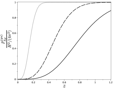
If we choose another window function, for example the Gaussian one Eq. (5), we have to perform the integrals that appear in Eq. (65) numerically. We have explicitly checked numerically that for values of the parameter in the Gaussian filter Eq. (5), the results obtained for the power spectrum are in very good agreement with those obtained with the step function filter, Eq. (67). In fact, when , the step filter is a very good approximation to the Gaussian filter. For example, this can be shown from the numerical results for the normalized spectrum obtained with the Gaussian filter, with the thermal contribution factor out, and whose results are shown in the figure 1.
IV.2 The thermal noise component for the power spectrum
Let us now compute the contribution in Eq. (53) depending on the thermal noise correlation function, given by the second term on the right-hand-side of Eq. (53). First note that the thermal noise correlation function Eq. (37), in momentum space and in terms of the variable , can be written as
| (69) |
where we have used the time variable written in terms of ,
| (70) |
together with
| (71) |
and the property of the Dirac delta-function,
| (72) |
where are the roots of .
From Eq. (69) and using the definition of the power spectrum Eq. (61), we then obtain the contribution to the power spectrum coming from the thermal noise source as given by
| (73) | |||||
Moss and Graham in Ref. GM have also found a similar result for the power spectrum, except that they have, instead of in their result, an effective dissipation coefficient . They then determine this effective dissipation coefficient by a matching procedure with the expected spectrum obtained for a flat space thermal field theory. Here, as we are going to see below, this is not necessary, since we are already determining the complete inflaton power spectrum, that includes both thermal and quantum noise sources.
For the relevant observational scale for the inflaton perturbations, which are produced in the late stages of inflation, the value of the argument in (73) can be taken as been small. Then, for example, we can approximate the integral appearing in Eq. (73) such that
| (74) | |||||
where is the Gamma function. Likewise, we can also use the asymptotic form for the Bessel function, i.e.,
| (75) |
By neglecting terms proportional to the slow-roll coefficients, with , such that we can take in the arguments of the Gamma functions in Eqs. (74) and (75), the thermal component for the power spectrum, Eq. (73), can finally be approximated as
| (76) | |||||
Note that the thermal spectrum is still approximately scale-invariant, as we would expect.
IV.3 The total power spectrum and relevant cosmological parameter results from observations
From the result for the quantum contribution to the power spectrum Eq. (67) and the result for the thermal contribution, Eq. (74) with Eq. (75), our result for the total power spectrum becomes,
| (77) |
which is conventionally evaluated at the moment of horizon crossing, . Note that in the zero temperature limit, , we also have that BMR () and the cold inflation result, Eq. (68) is re-obtained as expected. In the limit of and , we obtain , which is the original result obtained for warm inflation by Berera and Fang in Ref. firstWI . In the limit and we obtain that , which is the result found by Berera and Taylor in warmpert1 and also by Hall, Moss and Berera in warmpert2 .
From a perturbed Friedmann-Robertson-Walker metric with spatial curvature perturbation , it can be defined a gauge invariant comoving curvature perturbation as , which remains conserved throughout the evolution on super horizon scales. We can then choose a gauge, for example a spatially flat gauge, and write the curvature perturbation simple as liddlebook . Thus, from Eq. (77), we obtain the amplitude for the curvature perturbation during inflation, , as
| (78) |
where is a pivot scale liddlebook , , is the spectral index, defined by
| (79) |
where denotes the number of e-folds of inflation. These are all quantities that are read at the longest length scales of interest and taken to be those that first crossed the Hubble radius and which corresponds to the scales that crossed the horizon e-folds before the end of inflation. is between the usual canonical values, 50 and 60 e-folds Nespectra , whose specific value depends on the details of inflation and on the reheating phase after inflation. These will be the values of e-folds before the end of inflation that we will consider in the numerical analysis to be shown in section V below.
The most recent CMB radiation measurements from the WMAP nine years of accumulated data (WMAP9yr) gives for and , respectively, the values WMAP9yr : and , for the measurements from WMAP only. When the results from WMAP are combined with the results obtained from the extended CMB data (eCMB) (the CMB data coming from the Atacama Cosmology Telescope (ACT) and the South Pole Telescope (SPT)), from baryon acoustic oscillation (BAO) results and measurements for from galaxies surveys, it is obtained (assuming also contributions from tensor modes) and , respectively, which slight improves over the previous WMAP seven years of accumulated results (WMAP7yr), combined with similar databases (WMAP+BAO+), which have produced the results WMAP and .
Another cosmological parameter that helps to constrain many inflation type of models is the tensor to scalar curvature perturbation ratio, ,
| (80) |
where is the power spectrum of tensor metric perturbations, which for cold inflation is given by liddlebook
| (81) |
where is the reduced Planck mass. The value of is still poorly known, but an upper limit can be found from the observational data. The recent WMAP9yr results (WMAP+eCMB+BAO+) gives (at CL).
It has been shown in Ref. mohanty that in a thermal environment there can be a contribution to the tensor perturbation (81) coming from stimulated emission, if gravitons were in thermal equilibrium with the radiation bath. This effect would then imply a thermal enhancement factor in Eq. (81), just like the same factor also appearing in the quantum scalar perturbations, Eq. (67). The presence of this thermal enhancement factor in the tensor perturbation power spectrum depends whether the gravitational wave field is in thermal equilibrium with the radiation bath or not. In the original assumption made by Bhattacharya, Mohanty and Nautiyal in Ref. mohanty , inflation was considered to start in a state that was initially in a radiation dominated epoch, with temperature . Alternatively, if a thermal radiation bath develops in the course of inflation (as assumed in warm inflation) and the gravitons have enough time to equilibrate with the radiation bath and be strongly enough coupled to the particles in the radiation bath, then we also expect them to develop a thermal radiation-like spectrum, though in this case we would typically expect to be necessary at least temperatures for the radiation bath of order coles , which may be too high compared to the typical temperature scales during warm inflation, which are of the order of the Grand Unification (GUT) scale and below it. Nevertheless, the presence of the thermal enhancement factor appearing multiplicatively in Eq. (81) would increase the tensor to scalar curvature perturbation ratio and can potentially produce a much stronger constraint on nonisentropic inflation models than in the absence of this factor. Since some authors working on warm inflation have included explicitly in their studies this factor in the tensor curvature spectrum (see, for example, Refs. delCampo:2007cy ; Setare:2012fg ) and given the status of the presence of this term is unclear in the context of nonisentropic inflation in general, we will consider cases with and without the thermal enhancement factor included in the tensor curvature spectrum in the results to be presented below in section V, so both situations can be compared with the present observational constraint on .
The specialized expression for in the context of stochastic nonisentropic inflation model, with the thermal enhancement factor included in Eq. (81) (and with the spectra taken at the moment our current horizon scale crossed the de Sitter horizon during inflation, i.e., ) is then given by
| (82) |
where we have used the expression for the amplitude of scalar curvature perturbation Eq. (78), along with the slow-roll equation for coming from Eq. (45) and the equation defining the slow-roll coefficient , Eq. (46).
It is useful to check some of the limiting behaviors for with respect to the dissipation and temperature. The result for becomes more transparent if we instead look at the inverse ratio . Using that , we obtain (at ),
| (83) |
Taking for example the weak dissipation regime and for either or , we obtain , i.e., , which is the standard cold inflation result liddlebook . For and , we obtain that , i.e., , while in the case of not having the thermal enhancement factor in Eq. (82), or also when in (82), we obtain the warm inflation result for in the strong dissipation regime, . We can then conclude that even in the presence of the thermal enhancement factor in , for the weak dissipation regime the cold inflation result for is preserved independently of the value of the temperature for the thermal radiation bath. It is only in the strong dissipation regime that the ratio is affected by the dissipation, which makes smaller by a factor . This leads to an important aspect of warm inflation, making it possible to evade the so called Lyth bound Lyth (in particular, as observed in Ref. Cai:2010wt , this implies that large field inflation models do not necessarily yield a large tensor-to-scalar ratio). Therefore, thermal noises only affect scalar type curvature perturbations, but primordial gravitational waves (and associated tensor perturbations) are still originated from quantum vacuum fluctuations (though it may receive a correction dependent on the temperature, when in a thermal bath, because now the vacuum becomes a quantum statistical vacuum at some temperature and the gravitons can have a non zero occupation number, as shown in Ref. mohanty ).
For the sake of completeness, we also show here the limiting behaviors of in relation to and . Details concerning the derivation of , in the context of nonisentropic inflation in general, are given in the appendix A. From Eq. (79), taking the and limit, we obtain the expected result from cold inflation liddlebook ,
| (84) |
In the large and limit (and temperature independent dissipation), we recover the standard warm inflation result (e.g., from Hall, Moss and Berera Ref. warmpert2 ):
| (85) |
Finally, in the low dissipation limit, we obtain the first order correction for :
| (86) |
If we relax on the assumption of a power spectrum that is a pure power-law, like the one given in Eq. (78), and one admits a running spectral index, then we can write Kosowsky:1995aa
| (87) |
With the possibility of a running, the spectral index tends to be blue tilted, as opposite to a red tilt () in the case of no running. Some inflation models, like hybrid inflation, in fact prefer a blue tilted spectral index, while others, like chaotic inflation type of models, tend to be more red tilted. Observational data, however, are still not precise enough to give a definitive answer whether a running is favorable or not, with no statistically significant deviation from a pure power-law spectrum. For example, the WMAP9yr results for the running are only with less than significance WMAP9yr . Tensor mode amplitude and scalar running index parameter, when fitted together, give WMAP9yr : (at 95 CL), and (using the combined data from WMAP9yr+eCMB+BAO+). For the analysis and results to be presented in the next section, we have chosen to concentrate on the cases of no running of the spectrum, when contrasting the results obtained for nonisentropic inflation with the observational data.
V Results and constraints for nonisentropic inflation models from the observational data
Since the early releases of the WMAP CMBR results, a significant pressure has been put on inflation models. Both the spectral index and the tensor to scalar perturbation ratio results have shown to be able to exclude large classes of inflationary models. For example, hybrid inflation models are disfavored for predicting in general a too blue tilted spectrum, while simple chaotic polynomial type of potentials, in the case of cold inflation, even though they have a preference for a red tilted spectrum, they have been seen to poorly fit the observational data (though nonminimal coupling to gravity can make them compatible with the observational data WMAP9yr ). In particular, the recent WMAP9yr results already exclude (at the 68 CL) all simple chaotic cold inflation polynomial potentials , with power (see, for instance, figure 7 in Ref. WMAP9yr ).
Since most of the present constraints from the observational data have been applied most to cold inflation models, it is also important to have a throughout analysis of how general nonisentropic models withstand the recent observational data as well. Even though some previous works (see, e.g., Refs. WIreviews2 ; delCampo:2007cy ; delCampo:2010by ) have addressed the consistency of warm inflation with the observational data, only a few examples with very specific values of parameters were studied. A complete analysis covering larger regions of parameter space and ranging from cold to warm inflation is still missing. Since the larger pressure from the observational date are on chaotic polynomial type of inflation models, which by themselves represent an important class of inflaton potential models from a microscopic model building perspective, these are, therefore, the type of inflation models we will be interested in studying next.
In the following we will study nonisentropic chaotic inflation potential models with a generic potential of the form
| (88) |
where is a dimensionless parameter fixing the energy scale and we will consider the cases , and , which are the most common type of chaotic inflation potentials used, for example, in cold inflation studies in general.
Having fixed the class of inflaton potentials that we will analyze, we next need also to specify the dissipation coefficient appearing in the expressions. Nonisentropic inflation can be regarded as a two-fluid system when evaluating density perturbations, where both the inflaton and the radiation fluctuations are effectively coupled through the temperature dependence of the dissipation coefficient . It has then been shown in Ref. GM that because of this dependence of the dissipation coefficient on the temperature, the radiation perturbations can back react on the inflaton perturbations, generating undesirable growth modes. However, recently in Ref. MBR , it was found that intrinsic microscopic decay processes in the radiation bath itself can cause it to slight depart from equilibrium, giving rise to viscous dissipative effects in the radiation fluid itself. These viscous effects were then shown to be able to remove the growing modes and to lead to a power spectrum for the perturbations consistent with cases where the temperature was absent in . In this case, where the temperature can be neglected or it is absent in the expression for the dissipation coefficient, there are two representative forms of dissipation coefficient that can emerge and that are consistent with microscopic derivations (see, e.g., Refs. HR ; Ramos:2001zw ): a constant dissipation coefficient and a dissipation that has a quadratic dependence on the inflaton field, (these two forms of dissipation coefficients were also considered by the authors of the Refs. delCampo:2007cy ; delCampo:2010by in their studies involving warm inflation). These are, therefore, the two forms of dissipation coefficients we will use in our analysis, a constant dissipation coefficient, and also one proportional to the square of the inflaton amplitude, , with constant coefficient .
V.1 Cold and warm inflation dominated regions
As a preliminary study, let us first establish which regions of parameter space, in the plane defined by the dissipation coefficient over the Hubble parameter, , and by the temperature over the Hubble parameter, , the spectrum is dominated by quantum fluctuations or by thermal fluctuations. It has generically been accepted that warm inflation is determined by the parameters for which , considered the condition for which the thermal fluctuations dominate the spectrum. Warm inflation has also been considered in both the weak dissipation regime, and in the strong dissipation regime, . However, it has never been exactly established for which values of parameters we could really discriminate a cold inflation like spectrum, where quantum fluctuations dominate over the thermal ones, and the opposite regime of warm inflation.
We have determined in the previous section the contributions to the power spectrum coming from either quantum or thermal sources, with relevant results given by Eqs. (67) and (76), respectively. We can, thus, now determine the region of parameters where one contribution to the spectrum dominates over the other. In figure 2 we show the region of values of and for which , i.e., for which quantum fluctuations dominate over the thermal fluctuations, and for the opposite case, , i.e., for which thermal fluctuations dominate over the quantum fluctuations.
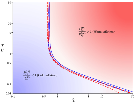
We believe that figure 2 is very illustrative of the conditions determining the different regimes that are possible in nonisentropic inflation models and it represents one of the main results in this paper. Figure 2 shows that there are no significant differences as regarding the dominating regions for each of the different polynomial forms for the inflaton potential, with little differences only between the cases . The figure also clearly shows that it is not always true that whenever we are in a warm inflation regime of a thermal fluctuation dominated spectrum. The thermal bath can have a temperature much larger than the Hubble parameter and we still be in a quantum fluctuation regime when . Likewise, the thermal bath can have in general a very low temperature compared to the Hubble parameter (or a temperature less than the one corresponding to the Hawking temperature) and the system can be in a warm inflation regime, where thermal fluctuations give the dominant contribution to the spectrum. These results come crucially from the fact that the quantum spectrum can depend on the temperature through a thermal enhancement factor, as shown in Eq. (67), which, as we have already discussed previously, comes from the consideration that in nonisentropic inflation models there is the presence of a radiation bath and that the inflaton fluctuations can be in thermal equilibrium with this produced radiation bath.
V.2 Observational constraints to the power spectrum
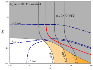
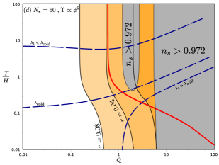
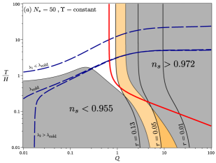
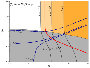
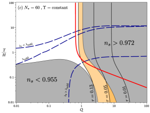
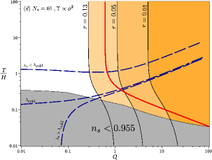
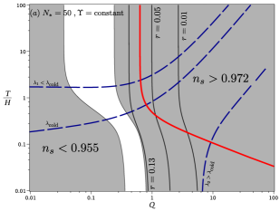
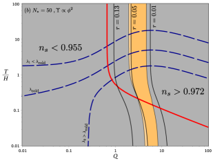
Having established in the previous subsection which are exactly the regions of parameter space where quantum or thermal fluctuations dominate, we turn now our attention to the question of the consistency of nonisentropic inflation in face of the recent observational data as coming from WMAP9yr. The observational parameters we test are the amplitude of the scalar curvature spectrum , the spectral index and the tensor to scalar curvature spectrum ratio , whose relevant expressions and data we have already given in section IV.3.
For the different forms of polynomial inflaton potentials considered, with powers (quadratic), (quartic) and (sextic) that we have tested, we have produced plots for the two canonical values of number of e-folds before the end of inflation, and . We have read (by numerically solving for) the spectrum of fluctuations leaving the horizon at these two values of . We have also produced sets of plots for the two cases of dissipation: a constant dissipation coefficient, , and for a dissipation with a quadratic dependence on the inflaton field, , with the constant coefficients and fixed by the numerical values taken for the ratio .
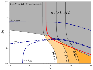
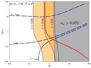
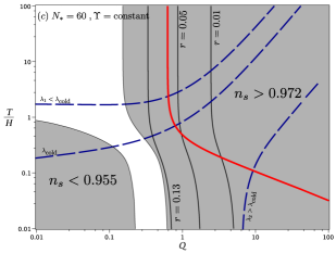
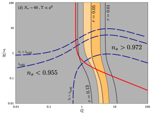
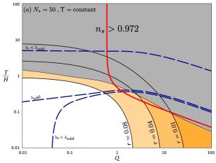
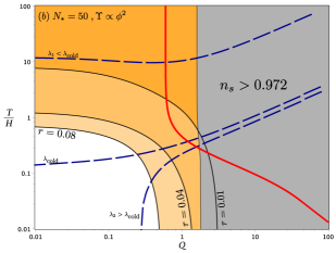
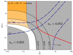
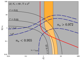
Instead of making the more traditional plots in a plane defined by the confidence levels (95 CL and 68 CL) for and and specify the inflation models (for different parameters) as points in this plane, we have chosen, instead, to represent the allowed regions in the plane . In the plane , we plot for each of the cases of inflaton potential, and dissipation coefficients, the permitted regions of parameter space consistent with the observational values of and . We have also draw lines of the inflaton potential parameter in Eq. (88) that are consistent with the amplitude of scalar perturbations . Different color shades in the plots will represent the different regions of parameter space that are allowed or not. The obtained results for each case are shown in the Figs. 3, 4 and 5, in the case of including the thermal enhancement factor in the expression for , Eq. (82), while in Figs. 6, 7 and 8 the thermal enhancement factor is absent.
In all the Figs. shown in this subsection, we have used the following representation and notation. The gray and white areas in the plots will indicate the regions of parameters not favored by the observational data, while the different shades of orange will indicate those regions of parameters that are favored. The gray regions are the regions outside the lower and upper values (from the mean) for the spectral index, with value taken as , obtained from the combined data coming from WMAP9yr+eCMB+BAO+ WMAP9yr . This value for is within the 68 CL region. The white areas are for (corresponding to a region disfavored by the observational data at the 95 CL), for the cases of the quartic and sextic inflaton potentials, or for (corresponding to a region disfavored by the observational data at the 68 CL), for the case of the quadratic inflaton potential. The different shades of orange, from light to dark, separated by thin black lines, indicate the regions of parameters that have decreasing values for the tensor to scalar curvature spectrum ratio . For the the quadratic inflaton potential (), we have (light orange), (medium orange) and (dark orange), respectively. For the quartic () and sextic () inflaton potentials, we have (light orange), (medium orange) and (dark orange), respectively. Results for the amplitude of scalar perturbations are given by the long-dashed thick blue lines. These long-dashed thick blue lines are for three different values of the parameter in Eq. (88) that are consistent with the central value for the amplitude of scalar perturbations, (WMAP9yr+eCMB+BAO+). is the value required by the pure cold inflation case ( and ), and are values below and above , respectively. All numerical values used for are indicated in the figure captions for each case. Finally, the thick red line in each of the plots separate the regions dominated by quantum fluctuations (region below the line), or dominated by thermal fluctuations (region above the line), according to figure 2.
In the figure 3 we have the results for the quadratic inflaton potential (). In the cold inflation regime, for both and , this potential is already ruled out by observations (at 68 CL) WMAP9yr in the pure cold inflation case (, ) and it is a viable potential in this case only at the 95 CL. However, for nonisentropic inflation, compatibility with observational data is recovered. For example, in the case of constant dissipation, compatible regions appear for low temperatures, , and strong dissipation, . In the case of inflaton field dependent dissipation, favored regions can run for all values of temperature, but for restrict values of dissipation, (for ), or (for ). Regions of thermal fluctuation domination are more favored in the inflaton field dependent dissipation case only, while for the constant dissipation case quantum fluctuation tend to give the most dominant contribution only.
In the figure 4 we have the results for the quartic inflaton potential (). This potential is ruled out in the pure cold inflation case (, ), for both the and cases, already at 95 CL when using the recent combined CMB data from from WMAP9yr+eCMB+BAO+ WMAP9yr . However, just like in the case for nonisentropic inflation, this potential can also become again compatible with the observational data. All panels in figure 4 show compatible regions with quantum and thermal fluctuations domination. However, thermal fluctuations (warm inflation) dominated regions are more favorable in the field dependent dissipation cases, panels (b) and (d). The cases of constant dissipation, panels (a) and (c), show, however, much smaller compatible regions with the observational data and that it happens only in a thin strip region of values ranging from somewhere in the range , at least in the presence of the thermal enhancement factor in Eq. (82) (see the results shown below, in the case when the enhancement factor in is not included).
In the figure 5 we have the results for the sextic inflaton potential (). This potential is completely ruled out in the pure cold inflation case (, ), for both the and cases, even when taking WMAP only results WMAP9yr . This inflaton potential is the most constrained one by the observational data even in the nonisentropic inflation case. In particular, in the case of constant dissipation (panels (a) and (c) in figure 5), it is discarded by not having regions compatible with the upper bound on , at 95 CL (again, just like in the case of the quartic potential, this situation can change when discarding the enhancement factor in , as we will discuss below). In the case of a dissipation coefficient that depends on the inflaton field (panels (b) and (d) in figure 5), a compatible region with the observational data only appears for a small strip of values of , ranging in between . Inside this range of , we find compatible regions for all values of temperature and also covering both quantum fluctuation dominated regions (that happens for ) and thermal fluctuation dominated regions (for ).
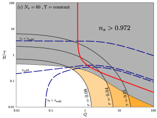
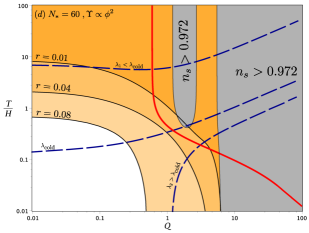
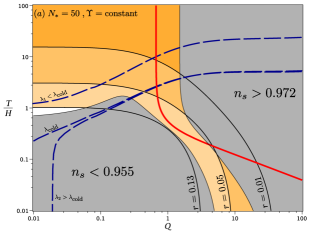
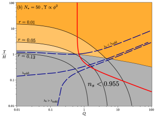
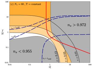
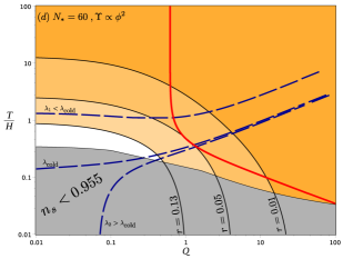
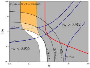
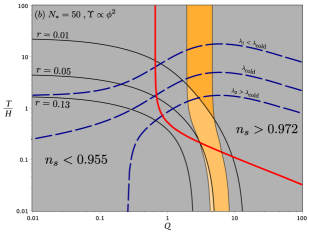
For the sake of comparison, in Figs. 6, 7 and 8 we show the parameter space behavior when we do not take into account the thermal enhancement term in Eq. (82), i.e., when considering a spectrum of gravitational waves that is decoupled from the thermal radiation bath generated during nonisentropic inflation. Note now that for all cases the region of parameters consistent with the observations increase, allowing as well larger regions for which (dark orange shaded regions). These results show that the cases of constant dissipation tend to favor more the quantum fluctuation dominated regime, with very small or completely absent regions of thermal fluctuation dominated regime (like for a sextic inflaton potential, ), while for a dissipation coefficient that depends on the inflaton field, we can have regions of parameters in both regimes. Note also that the larger region of favorable parameters appear when considering the quartic inflaton potential, with the sextic potential still being the most constrained case.
V.3 Planck results
As a final note, we notice that the recently released Planck results Ade:2013rta give for the tensor to scalar amplitude ratio the result at CL (when the high- CMB ACT+SPT data are added) and for the spectral index , while when including the Planck lensing likelihood gives and , and by also adding BAO data, it gives and . These values are to be compared with the ones we have used here, and (at CL), obtained from the combined data coming from WMAP9yr+eCMB+BAO+ WMAP9yr , which is quite consistent with those results from Planck. Therefore, all our results obtained previously remain fully valid when also accounting for the recent Planck data, indicating that the pressure on single field chaotic polynomial inflation models observed for cold inflation, does not hold in general for nonisentropic inflation models.
VI Conclusions
With the increasing precision that are reaching the cosmological parameters obtained from the observational data, considerable constraints are been put on many inflationary models. With the recent release of the accumulated nine years of WMAP data, combined with other CMB data from ACT and SPT and other astrophysical data coming from BAO and precise measurements of from large scale surveys, the simplest single field polynomial potential chaotic inflation models with quadratic and higher powers are ruled out at the 95 CL. Even simple monotonic inflation models appear disfavored at the 68 CL. These results, however, only apply to pure cold inflation models, in their most simple implementations and where the perturbation spectra is generated by quantum fluctuations only. In this work, we have analyzed a much larger class of inflation models, the nonisentropic inflation models. In these type of models the perturbation spectra is not sole determined by quantum fluctuations of the inflaton field, but because in this class of models a non negligible amount of radiation can be produced during inflation, thermal fluctuations can as well make a significant contribution to the power spectra. An example of a nonisentropic inflation model is warm inflation, where perturbation spectra come dominantly from thermal fluctuations. Warm inflation models are known to have a much less constrained parameter space and these models can be made compatible with the observational data. However, no study has been made to date in order to explore parameter regimes ranging from pure cold inflation to warm inflation. We have made this analysis in this work.
By appropriately making use of the stochastic inflation program, we have successfully been able to describe both cold and warm inflation concomitantly. This has allowed us to obtain the combined contributions to the power spectrum coming from both quantum and thermal fluctuations. From these results, we were able to fully determine regions of parameter space when quantum fluctuations give the dominant contribution, or the opposite regime, when thermal fluctuations dominate the spectrum.
Since the observational data is strongly constraining and also putting considerable pressure on polynomial chaotic inflation type of models, which are also the type of models more easily prone to a microscopic quantum field theory description, as far model building for inflation is concerned, we have concentrated our analysis on these type of inflation models. We have, thus, investigated the viability of the nonisentropic polynomial chaotic inflation models in face of the most recent results for the cosmological parameters, including the amplitude of scalar curvature perturbations, the spectral index for the scalar perturbations and the ratio of tensor to scalar perturbations. We have investigated the cases of a quadratic, quartic and a sextic inflaton potential. In all cases we have found that the presence of a radiation bath and dissipation in the inflaton dynamics (which are the characteristics of all nonisentropic inflation models) can lead to compatible regions of parameter space with the observational data, re-establishing the viability of these inflaton potential models.
Many characteristics of nonisentropic inflation models can be strongly dependent on the quantum field microphysics dynamics involved during inflation. These include, for example, the details of the model building, like how exactly the radiation bath is produced, the thermalization of the inflaton perturbations and the magnitude and dependence of the dissipation terms present during inflation. Even so, the approach we have adopted here is mostly model independent and our results can easily be extended to other type of inflation models, including, for example, hybrid inflation models, models motivated by string and superstring theories Cai:2010wt ; Cerezo:2012ub , loop quantum gravity motivated inflation models Herrera:2010yg , braneworld type of models Nozari:2009th ; BasteroGil:2011mr ; Herrera:2011zz , inflation models with nonstandard potentials Herrera:2012ep , among many others.
Appendix A Evaluation of the spectral index
In order to determine the expression for , it is useful to define the following derivatives in terms of the slow-roll parameters:
| (89) |
where . From the Friedmann equation for , we obtain
| (90) |
Another useful expression is
| (91) |
For a given mode with wavenumber , we can then write
| (92) |
Using also the equation for the entropy density in the slow-roll regime,
| (93) |
then, . Using also Eq. (91) combined with the previous ones, we obtain the relation
| (94) | |||||
Now we have to work out the term. Assuming , then
| (95) | |||||
Using Eq. (94), we obtain:
| (96) |
Using , we obtain:
| (97) |
Using and , we obtain from the above equation,
| (98) |
If we want to evaluate Eq. (94) in terms of slow-roll parameters, and , Eq. (92), we simply insert Eq. (98) in Eq. (94). Note that for the cases of no temperature dependence on the dissipation coefficient, then we would have in the above expressions. Likewise, for a constant dissipation, we would have . Analogously, we have:
| (99) |
and
| (100) |
Acknowledgements.
R.O.R. is partially supported by research grants from Conselho Nacional de Desenvolvimento Científico e Tecnológico (CNPq) and Fundação Carlos Chagas Filho de Amparo à Pesquisa do Estado do Rio de Janeiro (FAPERJ). L.A.S. was supported by Coordenação de Aperfeiçoamento de Pessoal de Nível Superior (CAPES).References
- (1) C. L. Bennett et al., 4-Year COBE DMR Cosmic Microwave Background Observations: Maps and Basic Results, Astrophys. J. 464, L1 (1996) [arXiv:astro-ph/9601067].
- (2) E. Komatsu et al., Seven-Year Wilkinson Microwave Anisotropy Probe (WMAP) Observations: Cosmological Interpretation, Astrophys. J. Suppl. 192 (2011) 18 [arXiv:1001.4538 [astro-ph.CO]]; D. Larson et al., Seven-Year Wilkinson Microwave Anisotropy Probe (WMAP) Observations: Power Spectra and WMAP-Derived Parameters, Astrophys. J. Suppl. 192 (2011) 16 [arXiv:1001.4635 [astro-ph.CO]].
- (3) G. Hinshaw, D. Larson, E. Komatsu, D. N. Spergel, C. L. Bennett, J. Dunkley, M. R. Nolta and M. Halpern et al., Nine-Year Wilkinson Microwave Anisotropy Probe (WMAP) Observations: Cosmological Parameter Results, arXiv:1212.5226 [astro-ph.CO].
- (4) A. R. Liddle and D. H. Lyth, Cosmological inflation and large scale structure, Cambridge University Press, Cambridge U.K. (2000).
- (5) A. Berera, I. G. Moss and R. O. Ramos, Warm Inflation and its Microphysical Basis, Rept. Prog. Phys. 72 (2009) 026901; [arXiv:0808.1855 [hep-ph]].
- (6) M. Bastero-Gil and A. Berera, Int. J. Mod. Phys. A 24 (2009) 2207. [arXiv:0902.0521 [hep-ph]].
- (7) A. N. Taylor and A. Berera, Perturbation spectra in the warm inflationary scenario, Phys. Rev. D 62 (2000) 083517 [arXiv:astro-ph/0006077];
- (8) L. M. H. Hall, I. G. Moss and A. Berera, Scalar perturbation spectra from warm inflation, Phys. Rev. D 69 (2004) 083525 [arXiv:astro-ph/0305015];
- (9) H. P. de Oliveira and S. E. Joras, On perturbations in warm inflation, Phys. Rev. D 64 (2001) 063513 [arXiv:gr-qc/0103089]; W. Lee and L. -Z. Fang, Correlated hybrid fluctuations from inflation with thermal dissipation, Phys. Rev. D 69 (2004) 023514 [astro-ph/0310856]; T. Matsuda, Evolution of the curvature perturbations during warm inflation, JCAP 0906 (2009) 002 [arXiv:0905.0308 [astro-ph.CO]].
- (10) M. Gleiser and R. O. Ramos, Microphysical approach to nonequilibrium dynamics of quantum fields, Phys. Rev. D 50 (1994) 2441 [arXiv:hep-ph/9311278].
- (11) A. Berera, M. Gleiser and R. O. Ramos, Strong dissipative behavior in quantum field theory, Phys. Rev. D 58 (1998) 123508 [arXiv:hep-ph/9803394].
- (12) A. Berera and R. O. Ramos, Dynamics of interacting scalar fields in expanding space-time, Phys. Rev. D 71 (2005) 023513 [arXiv:hep-ph/0406339].
- (13) A. Berera, I. G. Moss and R. O. Ramos, Local Approximations for Effective Scalar Field Equations of Motion, Phys. Rev. D 76 (2007) 083520 [arXiv:0706.2793 [hep-ph]].
- (14) I. G. Moss and C. Xiong, Non-gaussianity in fluctuations from warm inflation, JCAP 0704 (2007) 007 [arXiv:astro-ph/0701302].
- (15) C. Graham and I. G. Moss, Density fluctuations from warm inflation, JCAP 0907 (2009) 013 [arXiv:0905.3500 [astro-ph.CO]].
- (16) M. Bastero-Gil, A. Berera and R. O. Ramos, Shear viscous effects on the primordial power spectrum from warm inflation, JCAP 1107 (2011) 030 [arXiv:1106.0701 [astro-ph.CO]].
- (17) H. P. de Oliveira and R. O. Ramos, Dynamical system analysis for inflation with dissipation, Phys. Rev. D 57 (1998) 741 [arXiv:gr-qc/9710093].
- (18) W. Lee and L. Z. Fang, Mass density perturbations from inflation with thermal dissipation, Phys. Rev. D 59 (1999) 083503 [arXiv:astro-ph/9901195].
- (19) A. A. Starobinsky, in Field Theory, Quantum Gravity and Strings, Lecture Notes in Physics Vol. 246 (Springer, Berlin/Heidelberg, 1986), p. 107.
- (20) S. -J. Rey, Dynamics Of Inflationary Phase Transition, Nucl. Phys. B 284 (1987) 706.
- (21) A. S. Goncharov, A. D. Linde and V. F. Mukhanov, The Global Structure of the Inflationary Universe, Int. J. Mod. Phys. A 2 (1987) 561.
- (22) M. Sasaki, Y. Nambu and K. -i. Nakao, Classical Behavior Of A Scalar Field In The Inflationary Universe, Nucl. Phys. B 308 (1988) 868.
- (23) A. A. Starobinsky and J. Yokoyama, Equilibrium state of a selfinteracting scalar field in the De Sitter background, Phys. Rev. D 50 (1994) 6357 [astro-ph/9407016].
- (24) S. Winitzki and A. Vilenkin, Effective noise in a stochastic description of inflation, Phys. Rev. D 61 (2000) 8
- (25) N. D. Birrel and P. C. W. Davis, Quantum Fields in Curved Space (Cambridge University Press, Cambridge, 1982); L. E. Parker and D. J. Toms, Quantum Field Theory in Curved Spacetime, (Cambridge University Press, Cambridge, 2009).
- (26) A. Berera and L. -Z. Fang, Thermally induced density perturbations in the inflation era, Phys. Rev. Lett. 74 (1995) 1912 [astro-ph/9501024]; A. Berera, Thermal properties of an inflationary universe, Phys. Rev. D 54 (1996) 2519 [hep-th/9601134]; A. Berera, M. Gleiser and R. O. Ramos, Strong dissipative behavior in quantum field theory, Phys. Rev. D 58 (1998) 123508 [hep-ph/9803394]; A. Berera, Warm inflation at arbitrary adiabaticity: A Model, an existence proof for inflationary dynamics in quantum field theory, Nucl. Phys. B 585 (2000) 666 [hep-ph/9904409].
- (27) E. A. Calzetta and B.-L. B. Hu, Nonequilibrium Quantum Field Theory (Cambridge University Press, Cambridge, 2008).
- (28) M. Bastero-Gil, A. Berera and R. O. Ramos, Dissipation coefficients from scalar and fermion quantum field interactions, JCAP 1109 (2011) 033 [arXiv:1008.1929 [hep-ph]].
- (29) M. Bastero-Gil, A. Berera, R. O. Ramos and J. G. Rosa, General dissipation coefficient in low-temperature warm inflation, JCAP 1301 (2013) 016 [arXiv:1207.0445 [hep-ph]].
- (30) A. Berera and R. O. Ramos, The Affinity for scalar fields to dissipate, Phys. Rev. D 63 (2001) 103509 [hep-ph/0101049]; A. Berera and R. O. Ramos, Construction of a robust warm inflation mechanism, Phys. Lett. B 567 (2003) 294 [hep-ph/0210301].
- (31) M. Morikawa, Dissipation And Fluctuation Of Quantum Fields In Expanding Universes, Phys. Rev. D 42 (1990) 1027.
- (32) E. Calzetta and B. L. Hu, Quantum fluctuations, decoherence of the mean field, and structure formation in the early universe, Phys. Rev. D 52 (1995) 6770 [gr-qc/9505046]; E. A. Calzetta and S. Gonorazky, Primordial fluctuations from nonlinear couplings, Phys. Rev. D 55 (1997) 1812 [gr-qc/9608057]; A. Matacz, A New theory of stochastic inflation, Phys. Rev. D 55 (1997) 1860 [gr-qc/9604022].
- (33) S. Matarrese, M. A. Musso and A. Riotto, Influence of superhorizon scales on cosmological observables generated during inflation, JCAP 0405 (2004) 008 [hep-th/0311059].
- (34) A. Hosoya, M. Morikawa and K. Nakayama, Stochastic Dynamics Of Scalar Field In The Inflationary Universe, Int. J. Mod. Phys. A 4 (1989) 2613. Y. Nambu, Quantum to classical transition of density fluctuations in the inflationary model, Phys. Lett. B 276 (1992) 11; M. Bellini, H. Casini, R. Montemayor and P. Sisterna, Stochastic approach to inflation: Classicality conditions, Phys. Rev. D 54 (1996) 7172; T. Tanaka and M. -a. Sakagami, Classical nature of the inflaton field with selfinteraction, Prog. Theor. Phys. 100 (1998) 547 [gr-qc/9705054]; F. C. Lombardo and D. Lopez Nacir, Decoherence during inflation: The Generation of classical inhomogeneities, Phys. Rev. D 72 (2005) 063506 [gr-qc/0506051];
- (35) C. -H. Wu, K. -W. Ng, W. Lee, D. -S. Lee and Y. -Y. Charng, Quantum noise and a low cosmic microwave background quadrupole, JCAP 0702 (2007) 006 [astro-ph/0604292].
- (36) W. Lee, K. -W. Ng, I-C. Wang and C. -H. Wu, Trapping effects on inflation, Phys. Rev. D 84 (2011) 063527 [arXiv:1101.4493 [hep-th]].
- (37) M. Liguori, S. Matarrese, M. Musso and A. Riotto, Stochastic inflation and the lower multipoles in the CMB anisotropies, JCAP 0408 (2004) 011 [astro-ph/0405544].
- (38) I. G. Moss and C. M. Graham, Particle production and reheating in the inflationary universe, Phys. Rev. D 78 (2008) 123526 [arXiv:0810.2039 [hep-ph]].
- (39) K. Bhattacharya, S. Mohanty and R. Rangarajan, Temperature of the inflaton and duration of inflation from WMAP data, Phys. Rev. Lett. 96 (2006) 121302 [hep-ph/0508070].
- (40) V. F. Mukhanov, H. A. Feldman and R. H. Brandenberger, Theory of cosmological perturbations. Part 1. Classical perturbations. Part 2. Quantum theory of perturbations. Part 3. Extensions, Phys. Rept. 215 (1992) 203. B. A. Bassett, S. Tsujikawa and D. Wands, Inflation dynamics and reheating, Rev. Mod. Phys. 78 (2006) 537 [astro-ph/0507632]. K. A. Malik and D. Wands, Cosmological perturbations, Phys. Rept. 475 (2009) 1 [arXiv:0809.4944 [astro-ph]].
- (41) K. Bhattacharya, S. Mohanty and A. Nautiyal, Enhanced polarization of CMB from thermal gravitational waves, Phys. Rev. Lett. 97 (2006) 251301 [astro-ph/0607049]; M. Gasperini, M. Giovannini and G. Veneziano, Squeezed thermal vacuum and the maximum scale for inflation, Phys. Rev. D 48 (1993) 439 [gr-qc/9306015].
- (42) W. Zhao, D. Baskaran and P. Coles, Detecting relics of a thermal gravitational wave background in the early Universe, Phys. Lett. B 680 (2009) 411 [arXiv:0907.4303 [gr-qc]].
- (43) S. del Campo, R. Herrera and D. Pavon, Cosmological perturbations in warm inflationary models with viscous pressure, Phys. Rev. D 75 (2007) 083518 [astro-ph/0703604 [ASTRO-PH]].
- (44) M. R. Setare and V. Kamali, Tachyon Warm-Intermediate Inflationary Universe Model in High Dissipative Regime, JCAP 1208 (2012) 034 [arXiv:1210.0742 [hep-th]]; A. Deshamukhya and S. Panda, Warm tachyonic inflation in warped background, Int. J. Mod. Phys. D 18 (2009) 2093 [arXiv:0901.0471 [hep-th]]; M. A. Cid, S. del Campo and R. Herrera, Warm inflation on the brane, JCAP 0710 (2007) 005 [arXiv:0710.3148 [astro-ph]].
- (45) D. H. Lyth, What would we learn by detecting a gravitational wave signal in the cosmic microwave background anisotropy ?, Phys. Rev. Lett. 78 (1997) 1861 [hep-ph/9606387].
- (46) Y. -F. Cai, J. B. Dent and D. A. Easson, Warm DBI Inflation, Phys. Rev. D 83 (2011) 101301 [arXiv:1011.4074 [hep-th]].
- (47) A. Kosowsky and M. S. Turner, CBR anisotropy and the running of the scalar spectral index, Phys. Rev. D 52 (1995) 1739 [astro-ph/9504071].
- (48) S. del Campo, R. Herrera, D. Pavon and J. R. Villanueva, On the consistency of warm inflation in the presence of viscosity, JCAP 1008 (2010) 002 [arXiv:1007.0103 [astro-ph.CO]].
- (49) R. O. Ramos, Fine tuning solution for hybrid inflation in dissipative chaotic dynamics, Phys. Rev. D 64 (2001) 123510 [astro-ph/0104379].
- (50) R. Cerezo and J. G. Rosa, Warm Inflection, JHEP 1301 (2013) 024 [arXiv:1210.7975 [hep-ph]].
- (51) R. Herrera, Warm inflationary model in loop quantum cosmology, Phys. Rev. D 81 (2010) 123511 [arXiv:1006.1299 [astro-ph.CO]].
- (52) K. Nozari and B. Fazlpour, Non-Minimal Warm Inflation and Perturbations on the Warped DGP Brane with Modified Induced Gravity, Gen. Rel. Grav. 43 (2011) 207 [arXiv:0906.5047 [hep-th]].
- (53) M. Bastero-Gil, A. Berera and J. G. Rosa, Warming up brane-antibrane inflation, Phys. Rev. D 84 (2011) 103503 [arXiv:1103.5623 [hep-th]].
- (54) R. Herrera and E. San Martin, Warm-intermediate inflationary universe model in braneworld cosmologies, Eur. Phys. J. C 71 (2011) 1701 [arXiv:1108.1371 [gr-qc]].
- (55) R. Herrera and M. Olivares, Warm-Logamediate inflationary universe model, Int. J. Mod. Phys. D 21 (2012) 1250047 [arXiv:1205.2365 [gr-qc]].
- (56) P. A. R. Ade et al. [ Planck Collaboration], arXiv:1303.5082 [astro-ph.CO].