Analysis of the Min-Sum Algorithm for Packing and Covering Problems via Linear Programming

Abstract

Message-passing algorithms based on belief-propagation (BP) are successfully used in many applications including decoding error correcting codes and solving constraint satisfaction and inference problems. BP-based algorithms operate over graph representations, called factor graphs, that are used to model the input. Although in many cases BP-based algorithms exhibit impressive empirical results, not much has been proved when the factor graphs have cycles.

This work deals with packing and covering integer programs in which the constraint matrix is zero-one, the constraint vector is integral, and the variables are subject to box constraints. We study the performance of the min-sum algorithm when applied to the corresponding factor graph models of packing and covering LPs.

We compare the solutions computed by the min-sum algorithm for packing and covering problems to the optimal solutions of the corresponding linear programming (LP) relaxations. In particular, we prove that if the LP has an optimal fractional solution, then for each fractional component, the min-sum algorithm either computes multiple solutions or the solution oscillates below and above the fraction. This implies that the min-sum algorithm computes the optimal integral solution only if the LP has a unique optimal solution that is integral.

The converse is not true in general. For a special case of packing and covering problems, we prove that if the LP has a unique optimal solution that is integral and on the boundary of the box constraints, then the min-sum algorithm computes the optimal solution in pseudo-polynomial time.

Our results unify and extend recent results for the maximum weight matching problem by [Sanghavi et al.,’2011] and [Bayati et al., 2011] and for the maximum weight independent set problem [Sanghavi et al.’2009].

1 Introduction

We consider optimization problems over the integers called packing and covering problems. Many optimization problems can be formulated as packing problems including maximum weight matchings and maximum weight independent sets. Optimization problems such as minimum weight set-cover and minimum weight dominating set are special cases of covering problems. The input for both types of problems consists of an $m\times n$ zero-one constraint matrix $\mathbf{A}$, an integral constraint vector $\mathbf{b}$, an upper bound vector $\mathbf{X}\in\mathds{N}^{n}$, and a weight vector $\mathbf{w}\in\mathds{R}^{n}$. An integral vector $\mathbf{x}\in\mathds{N}^{n}$ is an integral packing if $\mathbf{0}\leq\mathbf{x}\leq\mathbf{X}$ and $\mathbf{A}\cdot\mathbf{x}\leq\mathbf{b}$. In a packing problem the goal is to find an integral packing that minimizes $\mathbf{w}^{T}\cdot\mathbf{x}$. An integral vector $\mathbf{x}\in\mathds{N}^{n}$ is an integral covering if $\mathbf{0}\leq\mathbf{x}\leq\mathbf{X}$ and $\mathbf{A}\cdot\mathbf{x}\geq\mathbf{b}$. In a covering problem the goal is to find an integral packing that maximizes $\mathbf{w}^{T}\cdot\mathbf{x}$.

Packing and covering problems generalize problems that are solvable in polynomial time (e.g., maximum matching) and problems that are NP-hard and even NP-hard to approximate (e.g., maximum independent set). The hardness of special cases of these problems imply that general algorithms for packing/covering problems are heuristic in nature. Two heuristics that are used in practice to solve such problems are linear programming (LP) and belief-propagation (BP).

Linear programming deals with optimizing a linear function over polyhedrons (subsets of the Euclidean space $\mathds{R}^{n}$) [BT97]. Perhaps the most naive way to utilize linear programming in this setting is to solve the LP relaxation of the integer problem (i.e., relax the restriction that $\mathbf{x}\in\mathds{N}^{n}$ to the restriction $\mathbf{x}\in\mathds{R}^{n}$). If the result happens to be integral, then we are lucky and we have found an optimal integral packing or covering. A great deal of literature deals with characterizing problems for which this method works well (e.g., works on total unimodularity [Sch98]). In fact, LP decoding of error correcting codes works in the same fashion and has been proven to work well in average [FWK05, ADS09].

Belief-propagation is an algorithmic paradigm that deals with inference over graphical models [Pea88]. The graphical model that corresponds to packing/covering problems is a bipartite graph that represents the zero-one matrix $\mathbf{A}$. We focus on a common variant of belief-propagation that is called the min-sum algorithm (or the max-product algorithm). In the variant we consider, the initial messages are all zeros and messages are not attenuated.

Our main result is a proof that the min-sum algorithm is not better than the heuristic based on linear programming. This proof holds for every instance of packing and covering problems described above with respect to the min-sum algorithm with zero initialization and no attenuation.

Previous Work.

Message-passing algorithms based on belief-propagation (BP) have been invented multiple times (see [Gal63, Vit67, Pea88]). Numerous papers report empirical results that demonstrate the usefulness of these algorithms for decoding error correcting codes, inference with noise, constraint satisfaction problems, and many other applications [Yed11]. It took a while until it was noticed that algorithms for decoding of Turbo codes [BGT93] and LDPC codes [Gal63] are special variants of BP [MMC98, Wib96].

In this paper we focus on a common variant of BP called the min-sum algorithm, and consider the case where messages are initialized to zero. The BP algorithm is a message-passing algorithm in which messages are sent along edges of a graph called the factor graph. The factor graph of packing/covering problems is a bipartite graph that represents that constraint matrix $\mathbf{A}$. In essence, value computed by the min-sum algorithm for $x_{i}$ equals the outcome of a dynamic programming algorithm over a path-prefix tree rooted at the vertex corresponding to the $i$th column of $\mathbf{A}$. Since dynamic programming computes an optimal solution over trees, the min-sum algorithm is optimal when the factor graph is a tree [Pea88, Wib96]. A major open problem is to analyze the performance of BP (or even the min-sum algorithm) when the factor graph is not a tree. Execution of algorithms based on BP over graphs that contain cycles is often referred to as loopy BP.

Recently, a few papers have studied the usefulness of the min-sum algorithm for solving optimization problems compared to linear programming. Such a comparison for the maximum weight matching problem appears in [BSS08, BBCZ11, SMW11] with respect to constraints of the form $\sum_{u\text{ neighbor of }v}x_{(u,v)}\leq 1$ for every vertex $v$. Loosely speaking, the main result that they show for maximum weighted matching is that the min-sum algorithm is successful if and only if the LP heuristic is successful. The sufficient condition states that if the LP relaxation has a unique optimal solution and that solution is integral, then the min-sum algorithm computes this solution in pseudo-polynomial time. The necessary condition states that if the LP relaxation has a fractional optimal solution, then the min-sum algorithm fails. In [SSW09], the min-sum algorithm for the maximum weighted independent set problem was studied with respect to constraints $x_{u}+x_{v}\leq 1$ for every edge $(u,v)$. They prove an analogous necessary condition and present a counter-example that proves that the sufficient condition (i.e., unique optimal solution for the LP that is integral) does not imply the success of the min-sum algorithm. The performance of the min-sum algorithm has been also studied for computing shortest $s$-$t$ paths [RT08] and min-cost flows [GSW12, BCMR13].

Our Results.

The results in this paper extend and generalize previous necessary conditions for the success of the min-sum algorithm. This necessary condition implies that, compared to the LP heuristic, the min-sum algorithm is not a better heuristic for solving packing and covering problems. Our contributions can be summarized as follows: (1) We consider a unified framework of packing and covering problems. Previous works deal with a zero-one constraint matrix $\mathbf{A}$ that has two nonzero entries in each column (for maximum weight matching [BSS08, BBCZ11, SMW11]) or two nonzero entries in each row (for maximum weight independent set [SSW09]). Our results hold with respect to any zero-one constraint matrix $\mathbf{A}$. (2) We allow box constraints, namely $x_{i}\in\{0,1,\ldots,X_{i}\}$. Previous results consider only zero-one variables. (3) Our oscillation results hold also when the LP relaxation has multiple solutions. To obtain such a result, we consider the set of optimal values computed by the min-sum algorithm at each variable (rather than declare failure if there are multiple optimal values). We compare these sets with the optimal solutions of the LP relaxation and show a weak oscillation between even and odd iterations. (4) The analogous result for covering LPs is obtained by a simple reduction (see Claim 3) that applies complementation; this reduction generalizes reductions from maximum matchings to minimum edge covers [SMW11]. (5) We present a unified proof method based on graph covers. This method also enables us to prove convergence of the min-sum algorithm under certain restrictions (see Theorem 17 in Appendix A).

Techniques.

The main challenge in comparing between the min-sum algorithm and linear programming is in finding a common structure that captures both algorithms. It turns out that graph covers are a common structure. Graph covers have been used previously to analyze iterative message passing algorithms [VK05, HE11]. In the context of optimization problems, $2$-covers have been used in [BBCZ11] to reduce matchings in general graphs to matchings in bipartite graphs [BSS08]. Bayati et al. [BBCZ11] write that their “proof gives a better understanding of the often-noted but poorly understood connection between BP and LP through graph covers.” We further clarify this connection by using higher order covers that capture fractional optimal LP solutions, as suggested by Ruozzi and Tatikonda [RT12]. Graph covers not only capture LP solutions but also solutions computed by the min-sum algorithm. In fact, the min-sum algorithm performs the same computation over any graph cover because it operates over a path-prefix tree of the factor graph. Hence we make the mental experiment in which the min-sum algorithm is executed over a graph cover in which all the basic feasible solutions are integral. We avoid the problems associated with loopy-BP by considering a graph cover, the girth of which is much larger than the number of iterations of the min-sum algorithm. Thus the execution of the min-sum algorithm is equivalent to a dynamic programming over subtrees induced by balls in the graph cover. This mental game justifies a dynamic programming interpretation of the outcome of the min-sum algorithm. The dynamic programming algorithm makes a “local” decision based on balls, the radius of which is twice the number of iterations. The LP solution, on the other hand, is a global solution.

The proof proceeds by creating “hybrid” solutions that either refute the (global) optimality of the LP solution or the (local) optimality of the dynamic programming solution over the ball in the graph cover.

2 Preliminaries

2.1 Graph Terminology and Algebraic Notation

Algebraic Notation.

We denote vectors in bold, e.g., $\mathbf{x},\mathbf{z}$. We denote the $i$th coordinate of $\mathbf{x}$ by $x_{i}$, e.g., $\mathbf{x}=(x_{1},\ldots,x_{n})$. For a vector $\mathbf{x}\in\mathds{R}^{n}$, let $\left\|\mathbf{x}\right\|_{1}\triangleq\sum_{i}\left|x_{i}\right|$ denote the $\ell_{1}$ norm of $\mathbf{x}$. The cardinality of a set $S$ is denoted by $\left|S\right|$. We denote by $[n]$ the set $\{0,1,2,...,n\}$ for $n\in\mathds{N}$. For a set $S\subseteq[n]$, we denote the projection of the vector $\mathbf{x}$ onto indices in $S$ by $\mathbf{x}_{S}\in\mathds{R}^{\left|S\right|}$ .

A vector is rational if all its components are rational. Similarly, a vector is integral if all its components are integers. A vector is fractional if it is not integral, i.e., at least one of its components is not an integer.

Let ${\mathbf{X}}\in\mathds{N}^{n}$ denote a non-negative integral vector. Denote the Cartesian product $[{X}_{1}]\times\cdots\times[{X}_{n}]$ by $\mathrm{ZBox}({\mathbf{X}})$. Similarly, denote the Cartesian product $[0,{X}_{1}]\times\cdots[0,{X}_{n}]$ by $\mathrm{RBox}({\mathbf{X}})$. Note that vectors in $\mathrm{ZBox}(\mathbf{X})$ are integral.

Graph Terminology.

Let $G=(V,E)$ denote an undirected simple graph. Let $\mathcal{N}_{G}(v)$ denote the set of neighbors of vertex $v\in V$ (not including $v$ itself). Let $\deg_{G}(v)$ denote the edge degree of vertex $v$ in a graph $G$, i.e., $\deg_{G}(v)\triangleq\lvert\mathcal{N}_{G}(v)\rvert$. For a set $S\subseteq V$ let $\mathcal{N}_{G}(S)\triangleq\bigcup_{v\in S}\mathcal{N}_{G}(v)$. A path in $G$ is a sequence of vertices such that there exists an edge between every two consecutive vertices in the sequence. A backtrack in a path is a subpath that is a loop consisting of two edges traversed in opposite directions, i.e., a subsequence $(u,v,u)$. All paths considered in this paper do not include backtracks. The length of a path is the number of edges in the path. We denote the length of a path $p$ by $\lvert p\rvert$. Let $d_{G}(r,v)$ denote the distance (i.e., length of a shortest path) between vertex $r$ and $v$ in $G$, and let $\mathrm{girth}(G)$ denote the length of the shortest cycle in $G$. Let $B_{G}(v,t)$ denote the set of vertices in $G$ with distance at most $t$ from $v$, i.e., $B_{G}(v,t)\triangleq\{u\in V\mid d_{G}(v,u)\leq t\}$.

The subgraph of $G$ induced by $S\subseteq V$ consists of $S$ and all edges in $E$, both endpoints of which are contained in $S$. Let $G_{S}$ denote the subgraph of $G$ induced by $S$. A subset $S\subseteq V$ is an independent set if there are no edges in the induced subgraph $G_{S}$. A graph $G=(V,E)$ is bipartite if $V$ is the union of two disjoint nonempty independent sets.

2.2 Covering and Packing Linear Programs

We consider two types of linear programs called covering and packing problems. In both cases the matrices are zero-one matrices and the constraint vectors are positive.

In the sequel we refer to the constraints $\mathbf{x}\in\mathrm{ZBox}(\mathbf{X})$ and $\mathbf{x}\in\mathrm{RBox}(\mathbf{X})$ as box constraints.

Definition 1.

Let $\mathbf{A}\in\{0,1\}^{m\times n}$ denote a zero-one matrix with $m$ rows and $n$ columns. Let $\mathbf{b}\in\mathds{R}_{+}^{m}$ denote a constraint vector, let $\mathbf{w}\in\mathds{R}^{n}$ denote a weight vector, and let $\mathbf{X}\in\mathds{N}^{n}$ denote a domain boundary vector.

1. The integer program $\operatorname*{arg\,max}\big{\{}\mathbf{w}^{T}\cdot\mathbf{x}~{}\big{|}~{}\mathbf{A}\cdot\mathbf{x}\leq\mathbf{b},~{}\mathbf{x}\in\mathrm{ZBox}(\mathbf{X})\big{\}}$ is called a packing IP, and denoted by PIP.

2. The integer program $\operatorname*{arg\,min}\big{\{}\mathbf{w}^{T}\cdot\mathbf{x}~{}\big{|}~{}\mathbf{A}\cdot\mathbf{x}\geq\mathbf{b},~{}\mathbf{x}\in\mathrm{ZBox}(\mathbf{X})\big{\}}$ is called a covering IP, and denoted by CIP.

3. The linear program $\operatorname*{arg\,max}\big{\{}\mathbf{w}^{T}\cdot\mathbf{x}~{}\big{|}~{}\mathbf{A}\cdot\mathbf{x}\leq\mathbf{b},~{}\mathbf{x}\in\mathrm{RBox}(\mathbf{X})\big{\}}$ is called a packing LP, and denoted by PLP.

4. The linear program $\operatorname*{arg\,min}\big{\{}\mathbf{w}^{T}\cdot\mathbf{x}~{}\big{|}~{}\mathbf{A}\cdot\mathbf{x}\geq\mathbf{b},~{}\mathbf{x}\in\mathrm{RBox}(\mathbf{X})\big{\}}$ is called a covering LP, and denoted by CLP.

2.3 Factor Graph Representation of Packing and Covering LPs

The belief-propagation algorithm and its variant called the min-sum algorithm deal with graphical models known as factor graphs (see, e.g., [KFL01]). In this section we review the definition of factor graphs that are used to model covering and packing problems.

Definition 2 (factor graph model of packing problems).

A quadruple $\langle G,\Psi,\Phi,\mathbf{X}\rangle$ is the factor graph model of PIP if:

• $G=(\mathcal{V}\cup\mathcal{C},E)$ is a bipartite graph that represents the zero-one matrix $\mathbf{A}$. The set of variable vertices $\mathcal{V}=\{v_{1},\ldots,v_{n}\}$ corresponds to the columns of $\mathbf{A}$, and the set of constraint vertices $\mathcal{C}=\{C_{1},\ldots,C_{m}\}$ corresponds to the rows of $\mathbf{A}$. The edge set is defined by $E\triangleq\{(v_{i},C_{j})\mid\mathbf{A}_{ji}=1\}$.

• The vector $\mathbf{X}\in\mathds{N}^{n}$ defines the alphabets that are associated with the variable vertices. The alphabet associated with $v_{i}$ equals $\{0,\ldots,X_{i}\}$.

• For each constraint vertex $C_{j}$, we define a packing factor function $\psi_{C_{j}}:\mathrm{ZBox}(\mathbf{X})\rightarrow\{0,-\infty\}$, defined by

  $$\psi_{C_{j}}(\mathbf{y}) \triangleq\begin{cases}0&\text{if }~{}\sum_{v_{i}\in\mathcal{N}_{G}(C_{j})}y_{i}\leq b_{j}\\ -\infty&\text{otherwise}\end{cases}$$ (1)

  We denote the set of factor functions $\{\psi_{C_{j}}\}_{j}$ by $\Psi$.

• For each variable vertex $v_{i}$, we define a variable function $\phi_{v_{i}}:[0,X_{i}]\rightarrow\mathds{R}$ defined by $\phi_{v_{i}}(\beta)\triangleq w_{i}\cdot\beta$. We denote the set of variable functions $\{\phi_{v_{i}}\}_{i}$ by $\Phi$.

We note that (1) One could define a factor graph for PLP; the only difference is that the alphabet associated with variable vertex $v_{i}$ is the real interval $[0,X_{i}]$, and the range of each factor function is $\mathrm{RBox}(\mathbf{X})$. (2) The factor functions are local in the sense that each constraint vertex $C_{j}$ can evaluate the value of $\psi_{C_{j}}$ based on the values of its neighbors.

A vector $\mathbf{x}\in\mathds{R}^{n}$ is viewed as an assignment to variable vertices in $\mathcal{V}$ where $x_{i}$ is assigned to vertex $v_{i}$. To avoid composite indices, we use $x_{v}$ to denote the value assigned to $v$ by the assignment $\mathbf{x}$. An integral assignment $\mathbf{x}$ is valid if it satisfies all the constraints, namely, $x_{i}\in[X_{i}]$ for every $i$ and $\mathbf{A}\cdot\mathbf{x}\leq\mathbf{b}$.

The factor graph model allows for the following equivalent formulation of the packing integer program:

$$\operatorname*{arg\,max}\big{\{}\sum_{v\in\mathcal{V}}\phi_{v}(x_{v})+\sum_{C\in\mathcal{C}}\psi_{C}(\mathbf{x})~{}\big{|}~{}\mathbf{x}\in\mathrm{ZBox}(\mathbf{X})\big{\}}.$$ (2)

If there exists at least one valid assignment, then this formulation is equivalent to the formulation:

$$\operatorname*{arg\,max}\big{\{}\sum_{v\in\mathcal{V}}\phi_{v}(x_{v})~{}\big{|}~{}\text{$\mathbf{x}$ is a valid integral assignment}\big{\}}.$$ (3)

We may define a factor graph model for covering problems in the same manner. The only difference is in the definition of the covering factor functions, namely,

$$\psi_{C}(y) \triangleq\begin{cases}0&\text{if $\sum_{v\in\mathcal{N}_{G}(C)}y_{v}\geq b_{C}$}\\ \infty&\text{otherwise}\end{cases}$$ (4)

Using this factor model, we can reformulate the covering integer program CIP by

$$\operatorname*{arg\,min}\big{\{}\sum_{v\in\mathcal{V}}\phi_{v}(x_{v})+\sum_{C\in\mathcal{C}}\psi_{C}(\mathbf{x})~{}\big{|}~{}\mathbf{x}\in\mathrm{ZBox}(\mathbf{X})\big{\}}.$$ (5)

One could define a factor graph model for general LP’s as well. Suppose the goal is to maximize the objective function. Then, for each constraint, the range of the factor function is $\{-\infty,0\}$. If the constraint $C$ is satisfied, then the value of $\psi_{C}$ is $0$; otherwise it is $-\infty$.

3 Min-Sum Algorithms for Packing and Covering Integer Programs

In this section we present the min-sum algorithm for solving packing and covering integer programs with zero-one constraint matrices. Strictly speaking, the algorithm for PIP is a max-sum algorithm, however we refer to these algorithms in general as min-sum algorithms. All the results in this section apply to any other equivalent algorithmic representation (e.g., max-product-type formulations). We first define the min-sum algorithms for PIPs and CIPs, and then state our main results.

3.1 The Min-Sum Algorithm

The min-sum algorithm for the packing integer program (PIP) is listed as Algorithm 1. The input to algorithm min-sum-packing consists of a factor graph model $\langle G,\Psi,\Phi,\mathbf{X}\rangle$ of a PIP instance and a number of iterations $t\in\mathds{N}$. Each iteration consists of two parts. In the first part, each variable vertex performs a local computation and sends messages to all its neighboring constraint vertices. In the second part, each constraint vertex performs a local computation and sends messages to all its neighboring variable vertices. Hence, in each iteration, two messages are sent along each edge.

Let $\mu_{v\rightarrow C}^{(t^{\prime})}(\beta)$ denote the message sent from a variable vertex $v\in\mathcal{V}$ to an adjacent constraint vertex $C\in\mathcal{C}$ in iteration $t^{\prime}$ under the assumption that vertex $v$ is assigned the value $\beta\in\{0,\ldots,X_{v}\}$. Similarly, let $\mu_{C\rightarrow v}^{(t^{\prime})}(\beta)$ denote the message sent from $C\in\mathcal{C}$ to $v\in\mathcal{V}$ in iteration $t^{\prime}$ assuming that vertex $v$ is assigned the value $\beta\in\{0,\ldots,X_{v}\}$. Denote by $\mu_{v}(\beta)$ the final value computed by variable vertex $v\in\mathcal{V}$ for assignment of $\beta\in\{0,\ldots,X_{v}\}$.

The initial messages (considered as the zeroth iteration) have the value zero and are sent along all the edges from the constraint vertices to the variable vertices. We refer to these initial messages as the zero initialization of the min-sum algorithm.

The algorithm proceeds with $t$ iterations. In Line 2a the message to be sent from $v$ to $C$ is computed by adding the previous incoming messages to $v$ (not including the message from $C$) and adding to it $\phi_{v}(\beta)$. In Line 2b the message to be sent from $C$ back to $v$ is computed. The constraint vertex $C$ considers all the possible assignments $\mathbf{z}$ to its neighbors in which $z_{v}=\beta$. In fact, only assignments that satisfy the constraint of $C$ and the box constraints of the neighbors of $C$ are considered. The message from $C$ to $v$ equals the maximum sum of the previous incoming messages (not including the message from $v$) among these assignments.

Finally, in Line 3 each vertex $v$ decides locally on its outcome $\hat{x}_{v}$. The maximum value $\mu_{v}^{\max}$ is computed, and the set $\delta_{v,t}$ of values that achieve the maximum is computed as well. The decision $\hat{x}_{v}$ of vertex $v$ equals the minimum or maximum value in $\delta_{v,t}$ depending on the parity of $t$. Here, we deviate from previous descriptions of the min-sum algorithm that declare failure if $\delta_{v,t}$ contains more than one element.

Algorithm 1 min-sum-packing$(\langle G,\Psi,\Phi,\mathbf{X}\rangle,t)$ - A min-sum algorithm for a PIP  $\operatorname*{arg\,max}\{\mathbf{w}^{T}\cdot\mathbf{x}~{}|~{}\mathbf{A}\cdot\mathbf{x}\leq\mathbf{b},~{}\mathbf{x}\in\mathrm{ZBox}(\mathbf{X})\}$. Given the factor graph model $\langle G,\Psi,\Phi,\mathbf{X}\rangle$ of the PIP and the number of iterations $t\in\mathds{N}$, outputs a vector $\hat{\mathbf{x}}\in\mathrm{ZBox}(\mathbf{X})$.

1. Initialize: For each $(v,C)\in E$ and $\beta\in\{0,\ldots,X_{v}\}$ do

   $$\mu_{C\rightarrow v}^{(0)}(\beta)\leftarrow 0$$

2. Iterate: For $t^{\prime}=1$ to $t$ do

   1. For each $(v,C)\in E$ and $\beta\in\{0,\ldots,X_{v}\}$ do {variable-to-constraint message}

      $$\mu_{v\rightarrow C}^{(t^{\prime})}(\beta)\leftarrow\phi_{v}(\beta)+\sum_{C^{\prime}\in\mathcal{N}(v)\setminus\{C\}}\mu^{(t^{\prime}-1)}_{C^{\prime}\rightarrow v}(\beta)$$

   2. For each $(v,C)\in E$ and $\beta\in\{0,\ldots,X_{v}\}$ do {constraint-to-variable message}

      $$\mu_{C\rightarrow v}^{(t^{\prime})}(\beta)\leftarrow\max\left\{\sum_{u\in\mathcal{N}(C)\setminus\{v\}}\mu^{(t^{\prime})}_{u\rightarrow C}(z_{u})\bigg{|}\mathbf{z}\in\mathrm{ZBox}(\mathbf{X})\text{ s.t. }z_{v}=\beta,\psi_{C}(\mathbf{z})=0\right\}$$

3. Decide: For each $v\in\mathcal{V}$ do

   1. For each $\beta\in\{0,\ldots,X_{v}\}$ do

      $$\mu_{v}(\beta)\leftarrow\sum_{C\in\mathcal{N}(v)}\mu_{C\rightarrow v}^{(t)}(\beta)$$

   2. $\mu^{\max}_{v}\triangleq\max\{\mu_{v}(\beta)\mid\beta\in[X_{v}]\}$

   3. $\delta_{v,t}\triangleq\{\beta\mid\mu_{v}(\beta)=\mu^{\max}_{v}\}$.

   4. $$\hat{x}_{v}\leftarrow \begin{cases}\max\{\beta\mid\beta\in\delta_{v,t}\}&\text{if $t$ is even}\\ \min\{\beta\mid\beta\in\delta_{v,t}\}&\text{if $t$ is odd}\end{cases}$$

   Return $\hat{\mathbf{x}}$

Algorithm min-sum-covering listed as Algorithm 2 is based on the following reduction of the covering LP to a packing LP as follows. It is easy to write a direct min-sum formulation of algorithm min-sum-covering.

Claim 3.

Let $\mathbf{d}\triangleq\mathbf{A}\cdot\mathbf{X}-\mathbf{b}\in\mathds{R}^{m}$, then

$$\operatorname*{arg\,min}\big{\{}\mathbf{w}^{T}\cdot\mathbf{z}~{}\big{|}~{}\mathbf{A}\cdot\mathbf{z}\geq\mathbf{b},~{}\mathbf{z}\in\mathrm{RBox}(\mathbf{X})\big{\}}=\mathbf{X}-\operatorname*{arg\,max}\big{\{}\mathbf{w}^{T}\cdot\mathbf{x}~{}\big{|}~{}\mathbf{A}\cdot\mathbf{x}\leq\mathbf{d},~{}\mathbf{x}\in\mathrm{RBox}(\mathbf{X})\big{\}}.$$

Proof.

Consider the mapping $\varphi(\mathbf{z})\triangleq\mathbf{X}-\mathbf{z}$. The mapping $\varphi$ is a one-to-one and onto mapping from the set $\{\mathbf{z}\in\mathrm{RBox}(\mathbf{X})\mid\mathbf{A}\cdot\mathbf{z}\geq\mathbf{b}\}$ to the set $\{\mathbf{x}\in\mathrm{RBox}(\mathbf{X})\mid\mathbf{A}\cdot\mathbf{x}\leq\mathbf{d}\}$. Moreover, the mapping $\varphi$ satisfies $\mathbf{w}^{T}\cdot\mathbf{z}=\mathbf{w}^{T}\cdot\mathbf{X}-\mathbf{w}^{T}\cdot\varphi(\mathbf{z})$, and the claim follows. ∎

Algorithm 2 min-sum-covering$(\langle G,\Psi,\Phi,\mathbf{X}\rangle,t)$ - a min-sum algorithm for a CIP $\operatorname*{arg\,min}\{\mathbf{w}^{T}\cdot\mathbf{z}~{}|~{}\mathbf{A}\cdot\mathbf{z}\geq\mathbf{b},~{}\mathbf{z}\in\mathrm{ZBox}(\mathbf{X})\}$. Given the factor graph model $\langle G,\Psi,\Phi,\mathbf{X}\rangle$ of the CIP and the number of iterations $t\in\mathds{N}$, outputs a vector $\hat{\mathbf{z}}\in\mathrm{ZBox}(\mathbf{X})$.

1. Let $\langle G,\Psi^{\prime},\Phi,\mathbf{X}\rangle$ denote the factor graph model for the PLP

   $$\operatorname*{arg\,max}\big{\{}\mathbf{w}^{T}\cdot\mathbf{x}~{}\big{|}~{}\mathbf{A}\cdot\mathbf{x}\leq\mathbf{d},~{}\mathbf{x}\in\mathrm{ZBox}(\mathbf{X})\big{\}},$$

   where $\mathbf{d}\triangleq\mathbf{A}\cdot\mathbf{X}-\mathbf{b}$.

2. Let $\hat{\mathbf{x}}$ denote the outcome of min-sum-packing$(\langle G,\Psi^{\prime},\Phi,\mathbf{X}\rangle,t)$

3. Return $\hat{\mathbf{z}}\triangleq\mathbf{X}-\hat{\mathbf{x}}$.

3.2 Main Results

Notation.

Let $\text{OPT}_{\text{LP}}$ denote the set of optimal solutions of the packing LP

$$\text{OPT}_{\text{LP}}\triangleq\operatorname*{arg\,max}\big{\{}\mathbf{w}^{T}\cdot\mathbf{x}~{}\big{|}~{}\mathbf{A}\cdot\mathbf{x}\leq\mathbf{b},\mathbf{x}\in\mathrm{RBox}(\mathbf{X})\big{\}}.$$

Let $\langle G,\Psi,\Phi,\mathbf{X}\rangle$ denote the factor graph model of this packing LP. Fix a variable vertex $r\in\mathcal{V}$ in the factor graph $G$ of the packing LP. Let $x^{\min}_{r}\triangleq\min\{x^{*}_{r}\mid\mathbf{x}^{*}\in\text{OPT}_{\text{LP}}\}$ and let $x^{\max}_{r}\triangleq\max\{x^{*}_{r}\mid\mathbf{x}^{*}\in\text{OPT}_{\text{LP}}\}$. Let $\delta^{\min}_{r,t}$ and $\delta^{\max}_{r,t}$ denote the minimum and maximum values in $\delta_{r,t}$, respectively.

The proof of the following theorem appears in Section 5.2.

Theorem 4 (weak oscillation).

Consider an execution of min-sum-packing$(\langle G,\Psi,\Phi,\mathbf{X}\rangle,t)$. For every variable vertex $r\in\mathcal{V}$ the following holds:

1. If $t$ is even, then $\max\{\beta\mid\beta\in\delta_{r,t}\}\geq x^{max}_{r}$.

2. If $t$ is odd, then $\min\{\beta\mid\beta\in\delta_{r,t}\}\leq x^{min}_{r}$.

Corollary 5.

If there exists an optimal solution $\mathbf{x}\in\text{OPT}_{\text{LP}}$ such that $x_{r}$ is not an integer, then $\hat{x}_{r}\geq\left\lceil x_{r}\right\rceil$ if the number of iterations $t$ is even, and $\hat{x}_{r}\leq\left\lfloor x_{r}\right\rfloor$ if $t$ is odd.

The following corollary implies that if algorithm min-sum-packing outputs the same value for a vertex in two consecutive iterations, then this value is the LP optimal value.

Corollary 6.

Let $t$ denote an even number and $s$ denote an odd number. If $\delta_{r,t}\cap\delta_{r,s}\neq\emptyset$, then $\delta_{r,t}\cap\delta_{r,s}$ contains a single element $\beta$ such that $x^{\min}_{r}=x^{\max}_{r}=\beta$.

Proof.

If $\beta\in\delta_{r,t}\cap\delta_{r,s}$, then by Theorem 4, $x^{\max}_{r}\leq\delta^{\max}_{r,t}=\beta=\delta^{\min}_{r,s}\leq x^{\min}_{r}$. ∎

Previous works on the min-sum algorithm for optimization problems define the case that $\delta_{r,t}$ contains more than one element as a failure. Under this restricted interpretation, Theorem 4 and Corollary 5 imply a necessary condition for the convergence of the min-sum-packing algorithm. Namely, $\text{OPT}_{\text{LP}}$ must contain a unique optimal solution and this optimal solution must be integral. Indeed, if $x^{\min}_{r}<x^{\max}_{r}$, then $\hat{x}_{r}$ oscillates above and below the interval $(x^{\min}_{r},x^{\max}_{r})$ between even and odd iterations.

Analogous results holds for covering problems. We state only the theorem that is analogous to Theorem 4. Redefine $\text{OPT}_{\text{LP}}$ so that it denotes the set of optimal solutions of the covering LP, i.e.,

$$\text{OPT}_{\text{LP}}\triangleq\operatorname*{arg\,min}\big{\{}\mathbf{w}^{T}\cdot\mathbf{x}~{}\big{|}~{}\mathbf{A}\cdot\mathbf{x}\geq\mathbf{b},\mathbf{x}\in\mathrm{RBox}(\mathbf{X})\big{\}}.$$

Let $\langle G,\Psi,\Phi,\mathbf{X}\rangle$ denote the factor graph model of the covering LP.

Theorem 7 (weak oscillation).

Consider an execution of min-sum-covering$(\langle G,\Psi,\Phi,\mathbf{X}\rangle,t)$. For every variable vertex $r\in\mathcal{V}$ the following holds:

1. If $t$ is even, then $\min\{\beta\mid\beta\in\delta_{r,t}\}\leq x^{min}_{r}$.

2. If $t$ is odd, then $\max\{\beta\mid\beta\in\delta_{r,t}\}\geq x^{max}_{r}$.

See Appendix A for a discussion of the convergence of the min-sum algorithm.

4 Graph Liftings

In this section we briefly review the definition of graph coverings, state a combinatorial characterization based on [RT12], and show how the girth can be arbitrarily increased.

4.1 Covering Maps and Liftings

Definition 8 (covering map [AL02]).

Let $G=(V,E)$ and $\tilde{G}=(\tilde{V},\tilde{E})$ denote finite graphs. A graph homomorphism $\pi:\tilde{G}\rightarrow G$ is a covering map if for every $\tilde{v}\in\tilde{V}$ the restriction of $\pi$ to neighbors of $\tilde{v}$ is a bijection to the neighbors of $\pi(\tilde{v})$.

We refer only to finite covering maps. The pre-image $\pi^{-1}(v)$ of a vertex $v$ is called the fiber of $v$. It is easy to see that all the fibers have the same cardinality if $G$ is connected. This common cardinality is called the degree or fold number of the covering map. If $\pi:\tilde{G}\rightarrow G$ is a covering map, we call $G$ the base graph and $\tilde{G}$ a lift of $G$. In the case where the fold number of the covering map is $M$, we say that $\tilde{G}$ is an $M$-lift of $G$.

(a) Base graph $G$.

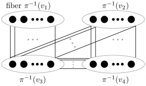
(b) An $M$-lift of $G$.

Figure 1: An $M$-lift of a base graph $G$: (1) fiber $\pi^{-1}(v_{i})$ consists of $M$ copies of $v_{i}$, and (2) for each edge $(v_{i},v_{j})$ in $G$, the set of edges between fibers $\pi^{-1}(v_{i})$ and $\pi^{-1}(v_{j})$ is a matching.

If $G$ is connected, then every $M$-lift of $G$ is isomorphic to an $M$-lift that is constructed as follows: (1) The vertex set is simply $\tilde{V}\triangleq V\times[M-1]$ and the covering map is the projection defined by $\pi\big{(}(v,i)\big{)}\triangleq v$. (2) For every $(u,v)\in E$, the edges in $\tilde{E}$ between the fibers of $u$ and $v$ constitute a matching.

The notion of $M$-lifts in graphs is extended to $M$-lifts of factor graph models in a natural manner. We denote a variable vertex in the fiber of by $\tilde{v}$ (so $\pi(\tilde{v})$ is denoted by $v$). Each variable vertex $\tilde{v}$ inherits the variable function of $v$, namely, $\tilde{w}_{\tilde{v}}\triangleq w_{v}$. Similarly, each constraint variable $\tilde{C}$ inherits the factor function of $\pi(\tilde{C})$. For brevity, we refer to the lifted factor graph model $\langle\tilde{G},\tilde{\Psi},\tilde{\Phi},\tilde{\mathbf{X}}\rangle$ of $\langle G,\Psi,\Phi,\mathbf{X}\rangle$ simply as the lift $\tilde{G}$ of a factor graph $G$.

An assignment $\mathbf{x}$ to the variable vertices $\mathcal{V}$ of a factor graph $G$ is extended to an assignment $\mathbf{\tilde{x}}$ over the lift $\tilde{G}$ simply by defining $\tilde{x}_{\tilde{v}}\triangleq x_{v}$. Note that this extension preserves the validity of assignments.

Every assignment $\mathbf{\tilde{x}}$ of an $M$-lift $\tilde{G}$ induces an assignment of the base graph $G$ that we call the average assignment. The average assignment $\mathrm{avg}(\tilde{\mathbf{x}})$ is defined by

$$\mathrm{avg}(\tilde{\mathbf{x}})_{v}\triangleq\frac{1}{M}\cdot\sum_{\tilde{v}\in\pi^{-1}(v)}\tilde{x}_{\tilde{v}}.$$ (6)

Consider an $M$-lift $\tilde{G}$ of the factor graph $G$ and a valid integral assignment $\mathbf{\tilde{x}}$ to $\tilde{G}$. By linearity, $\mathrm{avg}(\mathbf{\tilde{x}})$ is a rational valid assignment to $G$. The following theorem deals with the converse situation.

Theorem 9 (special case of [RT12, Theorem VII.2]).

For every rational feasible solution $\mathbf{x}$ of an LP, there exists an $M$, an $M$-lift $\tilde{G}$, and an integral valid assignment $\mathbf{\tilde{x}}$ to $\tilde{G}$ such that $\mathbf{x}=\mathrm{avg}(\mathbf{\tilde{x}})$.

Note that all the basic feasible solutions (extreme points) of the packing LP and the covering LP are rational.

4.2 Increasing Girth

The following proposition deals with obtaining lifts with large girth.

Proposition 10.

There exists a finite lift $\tilde{G}$ of $G$ such that $\mathrm{girth}(\tilde{G})\geq 2\cdot\mathrm{girth}(G)$.

Proof.

Given a graph $G=(V,E)$, we construct a $2^{\left|E\right|}$-lift $\tilde{G}=(\tilde{V},\tilde{E})$ as follows. Let $k=\left|E\right|$. The vertices in each fiber of $\tilde{G}$ are indexed by a binary string of length $k$. Index the edges in $E$ by $\{e_{1},\ldots,e_{k}\}$. For an edge $e_{i}=(u,v)$, the matching between the fiber of $u$ and the fiber of $v$ is induced simply by flipping the $i$’th bit in the index. Namely, $u_{\langle b_{1}\ldots b_{i}\ldots b_{k}\rangle}\mapsto v_{\langle b_{1}\ldots\overline{b_{i}}\ldots b_{k}\rangle}$.

Consider a cycle $\tilde{\gamma}$ in $\tilde{G}$ and its projection $\gamma$ in $G$. Each edge $e_{i}$ in $\gamma$ must appear an even number of times. Otherwise, the $i$’th bit is flipped an odd number of times in $\tilde{\gamma}$, and $\tilde{\gamma}$ can not be a cycle. It follows that $\mathrm{girth}(\tilde{G})\geq 2\cdot\mathrm{girth}(G)$. ∎

By applying Proposition 10 repeatedly, we have the following corollary.

Corollary 11.

Consider a graph $G$. Then for any finite $\ell\in\mathds{N}$ there exists a finite lift $\tilde{G}$ of $G$ such that $\mathrm{girth}(\tilde{G})\geq 2^{\ell}$.

5 Proof of Main Results

5.1 Min-Sum as a Dynamic Programming on Computation Trees

Given a graph $G=(V,E)$ and a vertex $r\in V$. The path-prefix tree of height $h$ is defined as follows.

Definition 12 (Path-Prefix Tree).

Let $\hat{V}$ denote the set of all paths with length at most $h$ without backtracks that start at vertex $r$. Let $\hat{E}\triangleq\big{\{}(p_{1},p_{2})\in\hat{V}\times\hat{V}\ \big{|}\ p_{1}\ \mathrm{is~{}a~{}prefix~{}of~{}}p_{2},~{}\lvert p_{1}\rvert+1=\lvert p_{2}\rvert\big{\}}$. The directed graph $(\hat{V},\hat{E})$ is called the path-prefix tree of $G$ rooted at vertex $r$ with height $h$, and is denoted by $\mathcal{T}_{r}^{h}(G)$.

We denote the zero-length path in $\hat{V}$ by $(r)$. The graph $\mathcal{T}_{r}^{h}(G)$ is obviously acyclic and is an out-tree rooted at $(r)$. Path-prefix trees of $G$ that are rooted in variable vertices are often called computation trees of $G$ or unwrapped trees of $G$.

We use the following notation. Vertices in $\mathcal{T}_{r}^{h}(G)$ are paths in $G$, and are denoted by $p$ and $q$ whereas variable vertices in $G$ are denoted by $u,v,r$. For a path $p\in\hat{V}$, let $t(p)$ denote the last vertex (i.e., target) of path $p$.

Consider a path-prefix tree $\mathcal{T}_{r}^{h}(G)$ of a factor graph $G=(\mathcal{V}\cup\mathcal{C},E)$. We denote the vertex set of $\mathcal{T}_{r}^{h}(G)$ by $\hat{\mathcal{V}}\cup\hat{\mathcal{C}}$, where $\hat{\mathcal{V}}$ denotes paths that end in a variable vertex, and $\hat{\mathcal{C}}$ denotes paths that end in a constraint vertex. Paths in $\hat{\mathcal{V}}$ are called variable paths, and paths in $\hat{\mathcal{C}}$ are called constraint paths. We attach variable functions $\hat{\phi}_{p}$ to variable paths $p$, and factor functions $\hat{\psi}_{q}$ to constraint paths; each vertex $p$ inherits the function of its endpoint. The box constraint for a variable path $p$ that ends at vertex $v$ is defined by $\hat{X}_{p}\triangleq X_{v}$.

In the following lemma, the min-sum-packing algorithm is interpreted as a dynamic programming algorithm over the path-prefix trees (see e.g., [GSW12, Section 2]).

Lemma 13.

Consider an execution of $\textsc{min-sum-packing}(\langle G,\Psi,\Phi,\mathbf{X}\rangle,t)$. Consider the computation tree $\mathcal{T}_{r}^{2t}(G)=(\hat{\mathcal{V}}\cup\hat{\mathcal{C}},\hat{E})$. For every variable vertex $r\in\mathcal{V}$ and $\beta\in\{0,\ldots,X_{r}\}$,

$$\mu_{r}(\beta)=\max\bigg{\{}\sum_{p\in\hat{\mathcal{V}}}\hat{\phi}_{p}(\hat{z}_{p})+\sum_{q\in\hat{\mathcal{C}}}\hat{\psi}_{q}(\hat{z}_{\mathcal{N}(q)})\bigg{|}~{}\forall p\in\hat{\mathcal{V}}.\hat{z}_{p}\in\mathrm{ZBox}(\hat{X}_{p}),~{}\hat{z}_{(r)}=\beta\bigg{\}}.$$

Definition 14 (optimal assignment).

We say that a valid assignment $\hat{z}$ to the variable paths in $\mathcal{T}_{r}^{2t}(G)$ is optimal if it maximizes the objective function $\sum_{p\in\hat{\mathcal{V}}}\hat{\phi}_{p}(\hat{z}_{p})+\sum_{q\in\hat{\mathcal{C}}}\hat{\psi}_{q}(\hat{z}_{\mathcal{N}_{\mathcal{T}}(q)})$.

Let $\text{OPT}_{\text{DP}}(r,t)$ denote the set of optimal valid assignments to the variable paths in $\mathcal{T}_{r}^{2t}(G)$. By Line 3c in algorithm min-sum-packing, the following corollary holds.

Corollary 15.

$\delta_{r,t}=\{z_{(r)}\mid\mathbf{z}\in\text{OPT}_{\text{DP}}(r,t)\}$.

5.2 Weak Oscillation of min-sum-packing - Proof of Theorem 4

Proof of Theorem 4.

We prove Part (1) of the Theorem. Fix an assignment $\mathbf{z}\in\text{OPT}_{\text{DP}}(r,t)$ such that $z_{(r)}=\delta^{\max}_{r,t}$. Fix an optimal solution $\mathbf{x}\in\text{OPT}_{\text{LP}}$ such that $x_{r}=x^{\max}_{r}$. Assume, for the sake of contradiction, that $t$ is even and that $z_{(r)}<x^{\max}_{r}$.

Without loss of generality, $\mathbf{x}$ is a basic feasible solution. By Theorem 9 and Corollary 11, for some $M$, there exists an $M$-lift $\langle\tilde{G},\tilde{\Psi},\tilde{\Phi},\tilde{\mathbf{X}}\rangle$ of $\langle G,\Psi,\Phi,\mathbf{X}\rangle$ such that: (i) there exists an integral valid assignment $\mathbf{\tilde{x}}$ for $\tilde{G}$ such that $\mathbf{x}=\mathrm{avg}(\mathbf{\tilde{x}})$, and (ii) $\mathrm{girth}(\tilde{G})>4t$.

The value of $x_{r}$ equals the average of $\tilde{\mathbf{x}}$ over the fiber of $r$. Let $\tilde{r}$ denote a vertex in the fiber of $r$ such that $\tilde{x}_{\tilde{r}}\geq x^{\max}_{r}$.

Let $B_{\tilde{G}}(\tilde{r},2t)$ denote the ball of radius $2t$ centered at $\tilde{r}$. Denote by $\tilde{G}_{B(\tilde{r},2t)}$ the subgraph of $\tilde{G}$ induced by $B_{\tilde{G}}(\tilde{r},2t)$. Because $\mathrm{girth}(\tilde{G})>4t$, $\tilde{G}_{B(\tilde{r},2t)}$ is a tree. It follows that $\tilde{G}_{B(\tilde{r},2t)}$ is isomorphic to the computation tree $\mathcal{T}_{r}^{2t}(G)$. Because $\mathbf{z}$ is an optimal valid assignment to $\mathcal{T}_{r}^{2t}(G)$, we can regard $\mathbf{z}$ also as an optimal valid assignment to the variable vertices in $\tilde{G}_{B(\tilde{r},2t)}$.

Because $z_{\tilde{r}}<x^{\max}_{r}$, the restriction of $\mathbf{\tilde{x}}$ to the variable vertices in $\tilde{G}_{B(\tilde{r},2t)}$ does not equal $\mathbf{z}$. Our goal is to obtain a contradiction by showing that either $\mathbf{z}$ is not an optimal assignment or there exists an optimal solution $\mathbf{y}\in\text{OPT}_{\text{LP}}$ such that $y_{r}>x^{\max}_{r}$. We show this by constructing “hybrid” integral solutions.

Let $\mathcal{E}\triangleq\{\tilde{u}\in B(\tilde{v},2t)\mid\frac{1}{2}\cdot d(\tilde{u},\tilde{r})\text{ is even}\}$. Similarly, let $\mathcal{O}\triangleq\{\tilde{u}\in B(\tilde{r},2t)\mid\frac{1}{2}\cdot d(\tilde{u},\tilde{r})\text{ is odd}\}$. Note that both $\mathcal{E}$ and $\mathcal{O}$ contain only variable vertices. We refer to $\mathcal{E}$ as the even layers and to $\mathcal{O}$ as the odd layers.

Let $\mathcal{F}$ denote the subgraph of $\tilde{G}_{B(\tilde{r},2t)}$ that is induced by: (i) the vertices $\tilde{u}\in\mathcal{E}$ such that $z_{\tilde{u}}<\tilde{x}_{\tilde{u}}$, (ii) the vertices $\tilde{u}\in\mathcal{O}$ such that $z_{\tilde{u}}>\tilde{x}_{\tilde{u}}$, and (iii) constraint vertices in $\tilde{G}_{B(\tilde{r},2t)}$. By definition, $\tilde{r}$ is a vertex in $\mathcal{E}$, and by our assumption $z_{\tilde{r}}<\tilde{x}_{r}$. Hence, $\tilde{r}\in\mathcal{F}$. Let $\mathcal{T}$ denote the connected component of $\mathcal{F}$ that contains $\tilde{r}$. We root $\mathcal{T}$ at $\tilde{r}$, and refer to $\mathcal{T}$ as an alternating tree.

A subtree $\mathcal{T}_{S}$ of $\mathcal{T}$ is a skinny tree if each constraint vertex chooses only one child and each variable vertex chooses all its children. Formally, a subtree $\mathcal{T}_{S}$ of $\mathcal{T}$ is a skinny tree if it is a maximal tree with respect to inclusion among all trees that satisfy (i) $\tilde{r}\in\mathcal{T}_{S}$, (ii) $\deg_{\mathcal{T}_{S}}(\tilde{C})=2$ for every constraint vertex $\tilde{C}$ in $\mathcal{T}_{S}$, and (iii) $\deg_{\mathcal{T}_{S}}(\tilde{u})=\deg_{\mathcal{T}}(\tilde{u})$ for every variable vertex $\tilde{u}$ in $\mathcal{T}_{S}$. We fix a skinny subtree $\mathcal{T}_{S}$ of $\mathcal{T}$ to obtain a contradiction.

For a subset of variable vertices $\tilde{A}\subseteq\tilde{\mathcal{V}}$, let $\tilde{w}(\tilde{A})\triangleq\sum_{\tilde{u}\in\tilde{A}}w_{u}$ (recall that the weight $w_{u}$ of a variable vertex $u$ in $G$ is given to each vertex $\tilde{u}$ in the fiber of $u$) . We claim that

$$\tilde{w}\big{(}\mathcal{T}_{S}\cap\mathcal{E}\big{)} \geq\tilde{w}\big{(}\mathcal{T}_{S}\cap\mathcal{O}\big{)},$$ (7)

To prove Equation (7), define an integral assignment $\mathbf{\tilde{y}}$ to variable vertices in $\tilde{\mathcal{V}}$ by

$$\tilde{y}_{\tilde{u}}\triangleq\begin{cases}\tilde{x}_{\tilde{u}}-1&\mathrm{if}~{}\tilde{u}\in\mathcal{T}_{S}\cap\mathcal{E}\\ \tilde{x}_{\tilde{u}}+1&\mathrm{if}~{}\tilde{u}\in\mathcal{T}_{S}\cap\mathcal{O}\\ \tilde{x}_{\tilde{u}}&\mathrm{otherwise.}\\ \end{cases}$$

Observe that $\mathbf{\tilde{y}}$ is a valid assignment for $\tilde{G}$. Indeed, all the box constraints are satisfied because we increment a value compared to $\tilde{x}_{u}$ only if $\tilde{x}_{\tilde{u}}<z_{\tilde{u}}$. Similarly, we decrement a value compared to $\tilde{x}_{u}$ only if $\tilde{x}_{\tilde{u}}>z_{\tilde{u}}$. In addition, we need to show that every constraint is satisfied by $\mathbf{\tilde{y}}$. Note that a constraint $\tilde{C}$ may have at most two neighbors that are variable vertices in the skinny tree; the rest of the neighbors retain the value assigned by $\mathbf{\tilde{x}}$. If a constraint $\tilde{C}$ is not a neighbor of a variable vertex in $\mathcal{T}_{S}$, then it is satisfied because $\mathbf{\tilde{x}}$ satisfies it. If a constraint $\tilde{C}$ has two neighbors that are variable vertices in $\mathcal{T}_{S}$, then one is incremented and the other is decremented. Overall, the constraint remains satisfied. Finally, suppose $\tilde{C}$ has only one neighbor in $\mathcal{T}_{S}$. Denote this neighbor by $\tilde{v}$. Then $\tilde{v}$ is a parent of $\tilde{C}$. If $\tilde{y}_{\tilde{v}}=\tilde{x}_{\tilde{u}}-1$, then clearly $\tilde{C}$ is satisfied by $\mathbf{\tilde{y}}$. If the value assigned to $\tilde{v}$ is incremented, then $\tilde{v}\in\mathcal{O}$ (i.e., an odd layer). This implies that the children of $\tilde{C}$ are in an even layer, the distance of which to the root is at most $2t$. Hence, the children of $\tilde{C}$ belong to the ball $B(\tilde{r},2t)$. Moreover, these children do not belong to the alternating tree (otherwise, one of its children would belong to the skinny tree). Thus, for each child $\tilde{u}$ of $\tilde{C}$ we have $z_{\tilde{u}}\geq\tilde{x}_{\tilde{u}}=\tilde{y}_{\tilde{u}}$. In addition, $z_{\tilde{v}}\geq\tilde{y}_{\tilde{v}}$. Hence, $\mathbf{z}\geq\mathbf{\tilde{y}}$ when restricted to the neighbors of $\tilde{C}$. Because $\mathbf{z}$ satisfies $\tilde{C}$, so does $\mathbf{\tilde{y}}$, as required. Because $\mathbf{\tilde{y}}$ is a valid assignment, $\mathrm{avg}(\mathbf{\tilde{y}})$ is a feasible solution of the packing LP. The optimality of $\mathbf{x}$ implies that $\mathbf{w}^{T}\cdot\mathbf{x}\geq\mathbf{w}^{T}\cdot\mathrm{avg}(\mathbf{\tilde{y}})$. By the definition of $\mathbf{\tilde{y}}$, we have

$$\mathbf{w}^{T}\cdot\big{(}\mathbf{x}-\mathrm{avg}(\mathbf{\tilde{y}})\big{)}=\frac{1}{M}\cdot\big{(}\tilde{w}(\mathcal{T}_{S}\cap\mathcal{E})-\tilde{w}(\mathcal{T}_{S}\cap\mathcal{O})\big{)},$$

and Equation (7) follows.

We now define an assignment $\theta$ to variable vertices in $\tilde{G}_{B(\tilde{r},2t)}$ by

$$\theta_{\tilde{u}}\triangleq\begin{cases}z_{\tilde{u}}+1&\mathrm{if}~{}\tilde{u}\in\mathcal{T}_{S}\cap\mathcal{E}\\ z_{\tilde{u}}-1&\mathrm{if}~{}\tilde{u}\in\mathcal{T}_{S}\cap\mathcal{O}\\ z_{\tilde{u}}&\mathrm{otherwise}\\ \end{cases}$$

We claim that $\theta$ is a valid integral assignment for $\tilde{G}_{B(\tilde{r},2t)}$. The proof is analogous to the proof that $\mathbf{\tilde{y}}$ is a valid assignment. By Equation (7), the value of $\theta$ is not less than the value of $\mathbf{z}$ since

$$\sum_{\tilde{u}\in\tilde{\mathcal{V}}\cap B_{\tilde{G}}(\tilde{r},2t)}\big{(}\phi_{\tilde{u}}(\theta_{\tilde{u}})-\phi_{\tilde{u}}(z_{\tilde{u}})\big{)}=\tilde{w}\big{(}\mathcal{T}_{S}\cap\mathcal{E}\big{)}-\tilde{w}\big{(}\mathcal{T}_{S}\cap\mathcal{O}\big{)}\geq 0.$$ (8)

Therefore, $\theta\in\text{OPT}_{\text{DP}}(r,t)$. However, $\theta_{r}>z_{r}=\delta^{\max}_{r,t}$, a contradiction. It follows that $\delta^{\max}_{r,t}\geq x^{\max}_{r,t}$ if $t$ is even.

The proof of Part (2) that $\delta^{\min}_{r,t}\leq x^{\min}_{r,t}$ for an odd $t$ is analogous to the proof that $\delta^{\max}_{r,t}\geq x^{\max}_{r,t}$ if $t$ is even. It requires the following modifications. (1) Fix $\mathbf{z}\in\text{OPT}_{\text{DP}}(r,t)$ such that $z_{(r)}=\delta^{\min}_{r}$ and $\mathbf{x}\in\text{OPT}_{\text{LP}}$ such that $x_{r}=x^{\min}_{r}$. (2) Assume towards a contradiction that $t$ is odd and $z_{(r)}>x_{r}$. (3) Pick $\tilde{r}$ so that $\tilde{x}_{\tilde{r}}\leq x_{r}$. (4) The forest $\mathcal{F}$ is induced by the following set of vertices: (i) the vertices $\tilde{u}\in\mathcal{E}$ such that $z_{\tilde{u}}>\tilde{x}_{\tilde{u}}$, (ii) the vertices $\tilde{u}\in\mathcal{O}$ such that $z_{\tilde{u}}<\tilde{x}_{\tilde{u}}$, and (iii) constraint vertices in $\tilde{G}_{B(\tilde{r},2t)}$. (5) Prove that the weight of even layers in the skinny tree is not greater than the weight of the odd layers. (6) The assignment $\mathbf{\tilde{y}}$ is defined so that it increments even layers and decrements odd layers. (7) The assignment $\theta$ is defined so that it decrements even layers and increments odd layers. ∎

Appendix A On Convergence of the Min-Sum Algorithm for Nonbinary Packing and Covering Problems

In Section 3.2 we showed that if the min-sum-packing algorithm outputs the same result in two consecutive iterations, then this result equals the optimal solution of the LP relaxation (see Corollary 6). On the other hand, even if the LP relaxation has a unique optimal solution and that solution is integral, then the min-sum-packing algorithm may not converge (see Sanghavi et al. [SSW09] for an example with respect to the maximum weight independent set problem).

Convergence of the min-sum algorithm was proved for the maximum weight $b$-matching and the minimum $r$-edge covering problems by Sanghavi et al. [SMW11] and Bayati et al. [BBCZ11]. They considered the zero-one integer program for maximum weight matching with the constraints $\sum_{e\ni v}x_{e}\leq 1$, and proved that after a pseudo-polynomial number of iterations, the min-sum algorithm converges to the optimal solution of the LP relaxation provided that it is unique and integral. The parameter that is used to bound the number of iterations is defined as follows.

Definition 16 ([SMW11]).

Given a polyhedron $\mathcal{P}\subseteq\mathds{R}^{n}$ and a cost vector $\mathbf{w}\in\mathds{R}^{n}$. Define $c(\mathcal{P},\mathbf{w})$ by

$$c(\mathcal{P},\mathbf{w}) \triangleq\min_{x\in\mathcal{P}\setminus\{x^{*}\}}\frac{\mathbf{w}^{T}\cdot(x^{*}-x)}{\|x^{*}-x\|_{1}},$$

where $x^{*}=\operatorname*{arg\,max}\{\mathbf{w}^{T}\cdot x\mid x\in\mathcal{P}\}$.

By definition, $C(\mathcal{P},\mathbf{w})\geq 0$, and $c(\mathcal{P},\mathbf{w})>0$ if and only the LP has a unique optimal solution. On the other hand, $c(\mathcal{P},\mathbf{w})\leq w_{\max}$, where $w_{\max}\triangleq\max\{w_{i}\mid 1\leq i\leq n\}$.

We generalize the convergence result of Sanghavi et al. [SMW11] to nonbinary packing and covering problems. For the sake of brevity we state the result for packing problems; the analogous result for covering problems holds as well.

Theorem 17.

Let $\mathcal{P}$ denote the polytope $\{\mathbf{x}\in\mathrm{RBox}(\mathbf{X})\mid\mathbf{A}\cdot\mathbf{x}\leq\mathbf{b}\}$. Assume that every column of $\mathbf{A}$ contains at most two $1$s. Assume that the packing LP $\operatorname*{arg\,max}\{\mathbf{w}^{T}\cdot\mathbf{x}~{}|~{}\mathbf{x}\in\mathcal{P}\}$ has a unique optimal solution $\mathbf{x}^{*}$ such that $x^{*}_{i}\in\{0,X_{i}\}$ for every $1\leqslant i\leqslant n$. Let $\langle G,\Psi,\Phi,\mathbf{X}\rangle$ denote the factor graph model of the packing LP. If $t>\frac{w_{\max}}{c(\mathcal{P},w)}+\frac{1}{2}$, then the output $\hat{\mathbf{x}}$ of Algorithm min-sum-packing$(\langle G,\Psi,\Phi\rangle,t)$ satisfies $\hat{\mathbf{x}}=\mathbf{x}^{*}$.

We first explain why the two restricting assumptions in Theorem 17 are useful.

Observation 18.

. If each column of $\mathbf{A}$ contains at most two $1$s, then the degrees of the variable vertices in the factor graph are at most $2$. Hence, the alternating skinny tree (as in the proof of Theorem 4) reduces to a path.

For every $M$-lift $\tilde{G}$ of a factor graph $G$, we define the polytope $\tilde{\mathcal{P}}=\{\tilde{\mathbf{x}}\in\mathrm{RBox}(\tilde{\mathbf{X}})\mid\tilde{\mathbf{A}}\cdot\tilde{\mathbf{x}}\leq\tilde{\mathbf{b}}\}$, where $\tilde{\mathbf{A}}$ and $\tilde{\mathbf{b}}$ are the constraint matrix and vector of the lifted factor graph.

Observation 19.

If the unique solution $\mathbf{x}^{*}$ of the packing LP satisfies $x^{*}_{i}\in\{0,X_{i}\}$ for every $1\leqslant i\leqslant n$, then $C(\tilde{\mathcal{P}},\tilde{\mathbf{w}})=C(\mathcal{P},\mathbf{w})$ for every $M$-lift $\tilde{G}$ of the factor graph $G$.

Proof of Theorem 17.  We focus on the case that $t$ is even; the proof for odd values of $t$ is analogous. The proof uses many of the notions used in the proof of Theorem 4 with modifications based on Observations 18 and 19, hence we reuse the same notations. Note that if $t$ is even and $x^{*}_{r}=X_{r}$, then Theorem 4 implies that $\delta^{\max}_{r,t}=X_{r}$, and hence $\hat{x}_{r}=x^{*}_{r}$, as required. Thus, we are left with the case that $x^{*}_{r}=0$ and wish to prove that $\delta^{\max}_{r,t}=0$ if $t$ is even.

Assume towards a contradiction that $\delta^{\max}_{r,t}>0$, and let $\mathbf{z}\in\text{OPT}_{\text{DP}}(r,t)$ denote an assignment such that $z_{(r)}=\delta^{\max}_{r,t}>0$. As in the proof of Theorem 4, we define an alternating tree in $\tilde{G}_{B(\tilde{r},2t)}$. However, the variable vertices in the even layers of the alternating tree satisfy $z_{\tilde{v}}>\tilde{x}^{*}_{\tilde{v}}$. Variables vertices in the odd layers of the alternating tree satisfy $z_{\tilde{v}}<\tilde{x}^{*}_{\tilde{v}}$. By Obs. 18, the skinny tree is simply a path that contains the root $\tilde{r}$.

Let $L$ denote the set of leaves of the skinny tree whose distance from $\tilde{r}$ is $2t$. Because the skinny tree is a path, it follows that $|L|\leq 2$.

Define an integral assignment $\mathbf{\tilde{y}}$ to variable vertices in $\tilde{\mathcal{V}}$ by

$$\tilde{y}_{\tilde{u}}\triangleq\begin{cases}\tilde{x}^{*}_{\tilde{u}}+1&\mathrm{if}~{}\tilde{u}\in(\mathcal{T}_{S}\cap\mathcal{E})\setminus L\\ \tilde{x}^{*}_{\tilde{u}}-1&\mathrm{if}~{}\tilde{u}\in\mathcal{T}_{S}\cap\mathcal{O}\\ \tilde{x}^{*}_{\tilde{u}}&\mathrm{otherwise.}\\ \end{cases}$$

As in the proof of Theorem 4, the assignment $\mathbf{\tilde{y}}$ is a valid assignment for $\tilde{G}$.

Assume that $L=\emptyset$. Since $\tilde{x}^{*}$ is a unique optimal assignment, it follows that

$$\tilde{w}\big{(}\mathcal{T}_{S}\cap\mathcal{O}\big{)} >\tilde{w}\big{(}(\mathcal{T}_{S}\cap\mathcal{E})\setminus L\big{)}.$$ (9)

Define

$$\theta_{\tilde{u}}\triangleq\begin{cases}z_{\tilde{u}}-1&\mathrm{if}~{}\tilde{u}\in\mathcal{T}_{S}\cap\mathcal{E}\\ z_{\tilde{u}}+1&\mathrm{if}~{}\tilde{u}\in\mathcal{T}_{S}\cap\mathcal{O}\\ z_{\tilde{u}}&\mathrm{otherwise.}\\ \end{cases}$$ (10)

As in the proof of Theorem 4, the assignment $\theta$ is a valid integral assignment for $\tilde{G}_{B(\tilde{r},2t)}$. But, Equation (9) implies that the assignment $\theta$ has a higher value than $\mathbf{z}$. This contradicts the optimality of $\mathbf{z}$.

Assume that $|L|=2$ (the proof for $|L|=1$ is similar). By the definition of $C(\tilde{\mathcal{P}},\tilde{\mathbf{w}})$ and by Obs. 19,

$$\frac{\tilde{\mathbf{w}}^{T}\cdot(\tilde{\mathbf{x}}^{*}-\mathbf{\tilde{y}})}{\|\tilde{\mathbf{x}}^{*}-\mathbf{\tilde{y}}\|_{1}}\geq C(\mathcal{P},\mathbf{w}).$$ (11)

Note that

$$\tilde{\mathbf{w}}^{T}\cdot(\tilde{\mathbf{x}}^{*}-\mathbf{\tilde{y}}) =\tilde{w}\big{(}\mathcal{T}_{S}\cap\mathcal{O}\big{)}-\tilde{w}\big{(}(\mathcal{T}_{S}\cap\mathcal{E})\setminus L\big{)},~{}\mathrm{and}$$

$$\|\tilde{\mathbf{x}}^{*}-\mathbf{\tilde{y}}\|_{1} =|\mathcal{T}_{S}|-|L|=2t-1.$$

It follows that

$$\tilde{w}\big{(}\mathcal{T}_{S}\cap\mathcal{O}\big{)}-\tilde{w}\big{(}(\mathcal{T}_{S}\cap\mathcal{E})\setminus L\big{)} \geq(2t-1)\cdot C(\mathcal{P},\mathbf{w}).$$ (12)

Consider the assignment $\theta$ defined in Equation (10). By Equation (12) we have

$$\sum_{\tilde{u}\in\tilde{\mathcal{V}}\cap B_{\tilde{G}}(\tilde{r},2t)}(\phi_{\tilde{u}}(\theta_{\tilde{u}})-\phi_{\tilde{u}}(z_{\tilde{u}})) =\tilde{w}\big{(}\mathcal{T}_{S}\cap\mathcal{O}\big{)}-\tilde{w}\big{(}\mathcal{T}_{S}\cap\mathcal{E}\big{)}$$

$$=\tilde{w}\big{(}\mathcal{T}_{S}\cap\mathcal{O}\big{)}-\tilde{w}\big{(}(\mathcal{T}_{S}\cap\mathcal{E})\setminus L\big{)}-\tilde{w}\big{(}L\big{)}$$

$$\geq(2t-1)\cdot C(\mathcal{P},\mathbf{w})-2\cdot w_{\max}.$$

Because $t>\frac{w_{\max}}{c(\mathcal{P},w)}+\frac{1}{2}$, it follows that the assignment $\theta$ has a higher value than $\mathbf{z}$. This contradicts the optimality of $\mathbf{z}$. It follows that $\delta^{\max}_{r,t}=0$ if $t$ is even. ∎

References

- [ADS09] S. Arora, C. Daskalakis, and D. Steurer, “Message passing algorithms and improved LP decoding,” in Proc. 41st Annual ACM Symp. Theory of Computing, Bethesda, MD, USA, pp. 3–12, 2009.
- [AL02] A. Amit and N. Linial, “Random graph coverings I: General theory and graph connectivity,” Combinatorica, vol. 22, no. 1, pp. 1–18, 2002.
- [BBCZ11] M. Bayati, C. Borgs, J. Chayes, and R. Zecchina, “Belief propagation for weighted b-matchings on arbitrary graphs and its relation to linear programs with integer solutions,” SIAM Journal on Discrete Mathematics, vol. 25, no. 2, pp. 989-–1011, 2011.
- [BCMR13] T. Brunsch, K. Cornelissen, B. Manthey, and H. Röglin, “Smoothed analysis of belief propagation for minimum-cost flow and matching,” in Proc. WALCOM: Algorithms and Computation, pp. 182-193, Springer Berlin Heidelberg, 2013.
- [BGT93] C. Berrou, A. Glavieux, and P. Thitimajshima, “Near Shannon limit error-correcting coding and decoding: Turbo-codes,” in Proc. IEEE Int. Conf. on Communications (ICC’93), Geneva, Switzerland, vol. 2, pp. 1064–1070, 1993.
- [BSS08] M. Bayati, D. Shah, and M. Sharma, “Max-product for maximum weight matching: Convergence, correctness, and LP duality,” IEEE Trans. Inf. Theory, vol. 54, no. 3, pp. 1241–-1251, Mar. 2008.
- [BT97] D. Bertsimas and J. N. Tsitsiklis, Introduction to linear optimization. Athena Scientific, 1997.
- [HE11] N. Halabi and G. Even, “On decoding irregular Tanner codes with local-optimality guarantees,” CoRR, http://arxiv.org/abs/1107.2677, Jul. 2011.
- [FWK05] J. Feldman, M. J. Wainwright, and D. R. Karger, “Using linear programming to decode binary linear codes,” IEEE Trans. Inf. Theory, vol. 51, no. 3, pp. 954–-972, Mar. 2005.
- [Gal63] R. G. Gallager, Low-Density Parity-Check Codes. MIT Press, Cambridge, MA, 1963.
- [GSW12] D. Gamarnik, D. Shah, and Y. Wei, “Belief propagation for min-cost network flow: Convergence and correctness,” Operations Research, vol. 60, no. 2, pp. 410–428, Mar.-Apr. 2012.
- [KFL01] F. R. Kschischang, B. J. Frey, and H.-A. Loeliger, “Factor graphs and the sum-product algorithm,” IEEE Trans. Inf. Theory, vol. 47, no. 2, pp. 498–519, Feb. 2001.
- [MMC98] R. J. McEliece, D. J. C. MacKay, and J.-F. Cheng, “Turbo decoding as an instance of pearl’s ‘belief propagation’ algorithm,” IEEE J. Select. Areas Commun., vol. 16, no. 2, pp. 140–152, Feb. 1998.
- [Pea88] J. Pearl, Probabilistic reasoning in intelligent systems: networks of plausible inference. Morgan Kaufmann, 1988.
- [RT08] N. Ruozzi and S. Tatikonda, “s-t paths using the min-sum algorithm,” in Proc. of the 46th Allerton Conference on Communication, Control, and Computing, Monticello, Illinois, USA, pp. 918–921, 2008.
- [RT12] N. Ruozzi and S. Tatikonda, “Message-passing algorithms: Reparameterizations and splittings,” CoRR, abs/1002.3239, v3, Dec. 2012.
- [Sch98] A. Schrijver, Theory of linear and integer programming. Wiley-Interscience, New York, NY, 1998.
- [SMW11] S. Sanghavi, D. Malioutov, and A. Willsky, “Belief propagation and LP relaxation for weighted matching in general graphs,” IEEE Trans. Inf. Theory, vol. 57, no. 4, pp. 2203 –2212, Apr. 2011.
- [SSW09] S. Sanghavi, D. Shah, and A.S. Willsky, “Message passing for maximum weight independent set,” IEEE Trans. Inf. Theory, vol. 55, no. 11, pp. 4822 –4834, Nov. 2009.
- [Vit67] Andrew Viterbi, “Error bounds for convolutional codes and an asymptotically optimum decoding algorithm,” IEEE Trans. Inf. Theory, vol. 13, no. 2, pp. 260–269, Apr. 1967.
- [VK05] P. O. Vontobel and R. Koetter, “Graph-cover decoding and finite-length analysis of message-passing iterative decoding of LDPC codes,” CoRR, http://www.arxiv.org/abs/cs.IT/0512078, Dec. 2005.
- [Wib96] N. Wiberg, “Codes and decoding on general graphs”, Ph.D. dissertation, Linköping University, Linköping, Sweden, 1996.
- [Yed11] J. S. Yedidia, “Message-passing algorithms for inference and optimization,” J. Stat. Phys., vol. 145, no. 4, pp. 860–890, Nov. 2011.