Detection of fast transients with radio interferometric arrays

Abstract

Next-generation radio arrays, including the SKA and its pathfinders, will open up new avenues for exciting transient science at radio wavelengths. Their innovative designs, comprising a large number of small elements, pose several challenges in digital processing and optimal observing strategies. The Giant Metre-wave Radio Telescope (GMRT) presents an excellent test-bed for developing and validating suitable observing modes and strategies for transient experiments with future arrays. Here we describe the first phase of the ongoing development of a transient detection system for GMRT that is planned to eventually function in a commensal mode with other observing programs. It capitalizes on the GMRT’s interferometric and sub-array capabilities, and the versatility of a new software backend. We outline considerations in the plan and design of transient exploration programs with interferometric arrays, and describe a pilot survey that was undertaken to aid in the development of algorithms and associated analysis software. This survey was conducted at 325 and 610 MHz, and covered 360 deg² of the sky with short dwell times. It provides large volumes of real data that can be used to test the efficacies of various algorithms and observing strategies applicable for transient detection. We present examples that illustrate the methodologies of detecting short-duration transients, including the use of sub-arrays for higher resilience to spurious events of terrestrial origin, localisation of candidate events via imaging and the use of a phased array for improved signal detection and confirmation. In addition to demonstrating applications of interferometric arrays for fast transient exploration, our efforts mark important steps in the roadmap toward SKA-era science.

1 Introduction

The transient Universe has remained a major astrophysical frontier over the past few decades. Transient phenomena are known on time scales ranging from as short as sub-nano seconds to years or longer, thus spanning almost 20 orders of magnitude in time domain. Such emission is thought to be likely indicators of explosive or dynamic events and hence provide enormous potential to uncover a wide range of new astrophysics (e. g. Cordes et al. 2004b).

While the transient sky at high energies (X- and $\gamma$-rays), and to some extent at optical wavelengths, are routinely monitored for transient and variable phenomena by a number of wide field-of-view instruments, it remains a largely uncharted territory at radio wavelengths. Most previous high-sensitivity radio surveys (for pulsars and transients) have used large single dishes which, by definition, have relatively narrow fields-of-view. In addition, for the case of detection of short-duration transients (“fast transients”, time scales of $\sim$microseconds to $\sim$seconds), there have been additional challenges such as the large signal processing overheads arising from the need to correct for effects such as dispersion, and the ever-increasing number of radio frequency interference sources. These challenges have limited the scope of rigorous explorations of the radio transient sky.

There are now a suite of new radio facilities in the design, construction or commissioning stages, many of which will offer wide field-of-view capabilities and thus open up new avenues of discovery. These are either multi-element radio arrays with moderate to large number of small-sized elements (dishes), or those comprising elements with natively wide field-of-view (i. e. aperture arrays). Examples include the newly operational Low Frequency Array (LOFAR) and the Murchison Widefield Array (MWA), as well as upcoming SKA pathfinder instruments, viz. the Australian SKA Pathfinder (ASKAP) in Western Australia and MeerKAT in South Africa (Stappers et al., 2011; Tingay et al., 2012; Johnston et al., 2007; Booth et al., 2009). In principle, these instruments can provide large field of view (FoV) observations; however, they also present significant challenges in terms of the associated signal processing costs. Fortuitously, with the recent advances in affordable super computing and the use of graphics processing units in astronomical computing, this is fast becoming less of a challenge (e.g. Barsdell et al., 2010; Magro et al., 2011). Therefore, optimistically, the availability of such next-generation arrays, together with appropriate instrumentation and suitable data archiving and processing strategies, can potentially revolutionize our knowledge of the transient radio sky in the coming decades.

The scientific potential of radio transients has been well underscored in a number of recent reviews (e.g. Cordes et al., 2004b; Cordes, 2009; Fender & Bell, 2011; Bhat, 2011). A wide variety of transient phenomena are known at radio wavelengths. While pulsar radio emission time scales range from milliseconds (sub-pulses) to nanoseconds (giant pulses), phenomena such as solar or stellar bursts, flares from Jupiter-like planets and brown dwarfs, micro-quasar emission, and gamma-ray burst (GRB) afterglows are of much longer durations (e.g. Chandra & Frail, 2011). Some known radio transients have been discovered in follow-up observations of higher-energy detections; for example, gamma-ray burst afterglows and periodic pulsations from magnetars (Camilo et al., 2006; Levin et al., 2010). Other discoveries include transient sources in the direction of the Galactic Centre (GC) (Hyman et al., 2005; Bower et al., 2007; Roy et al., 2010) found through time-resolved VLA imaging of the GC, rotating radio transients (RRATs) found in transient searches of archival pulsar surveys (McLaughlin et al., 2006; Keane & McLaughlin, 2011), and the possibly extragalactic millisecond bursts reported by Lorimer et al. (2007) and Keane et al. (2012).

A distinction is often made between “slow” versus “fast” transients in the context of radio astronomy (cf. Cordes, 2009); slow transients can be detected through standard imaging of brief or long time integrations, while fast transients require data collection with sufficiently high time and frequency resolution to correct for dispersive delays before detection is attempted. This paper is concerned with the detection of fast transients. These are often linked to coherent radiation processes and, frequently, to sources in extreme matter states (e.g. Cordes et al., 2004a). They are affected by plasma propagation effects such as dispersion and, if the source is compact, by multi-path scattering and/or scintillation by the intervening media; hence, they may also serve as excellent probes of such media.

As noted earlier, impulsive radio frequency interference (RFI) can potentially mimic signatures of real signals, and their frequent occurrence may impact an observation’s sensitivity, thereby making weaker signals difficult to detect (e.g. Bhat et al., 2005). Interferometric instruments offer several unique advantages here. The distributed nature of array elements and long baselines can be exploited to identify and eliminate a wide range of RFI-generated transients. For example, voltage data can be correlated between elements to find fringes for the pulse, hence obtaining a sky position and localizing the detection. Most ongoing fast transient explorations, with the exception of the VLBA-based V-FASTR project (Wayth et al., 2011) and the LOFAR pulsar survey project (Coenen et al., 2012), use large single-dish instruments such as Parkes and Arecibo (Deneva et al., 2009; Burke-Spolaor et al., 2011), which offer none of those advantages, both because of their lower resilience to RFI and also because the data are typically pre-processed prior to recording.

Despite the clear advantages of interferometric transient searches, exploiting such arrays will require considerable planning and exploratory research. As neither of the conventionally employed observing strategies, such as incoherent (i.e. phase-insensitive) addition of antenna signals or a single phased-up array, are optimal for conducting large sky surveys, some new strategies will need to developed and experimented in order to fully exploit array instruments (e.g. Janssen et al., 2009; Stappers et al., 2011; Coenen et al., 2012; Rubio-Herrera et al., 2013). Recently, Macquart (2011) and Colegate & Clarke (2011) approached the problem from the point of optimizing large-sky surveys within the context of next-generation array instruments including the SKA, and both advocate incoherent combination of antenna signals as optimal strategies to achieve the highest detectable event rates. Existing arrays (e. g. GMRT, VLBA, LOFAR) can meanwhile demonstrate effective strategies that will be applicable when next-generation arrays are constructed.

A number of salient features make the GMRT (Swarup et al., 1991) a powerful test-bed in this context. This low-frequency array of 30 x 45-m dishes, operating at 5 different frequency bands in the range 0.15 to 1.5 GHz and with an effective collecting area ${\rm A_{eff}}\sim$3% SKA, offers several unique design features. Its moderate number of elements, relatively long baselines (up to $\sim$25 km) and sub-array capabilities make it an excellent analog for SKA-like platforms. Furthermore, GMRT’s new software backend (Roy et al., 2010) allows raw voltage data from individual array elements to be rerouted to software-based processing systems.

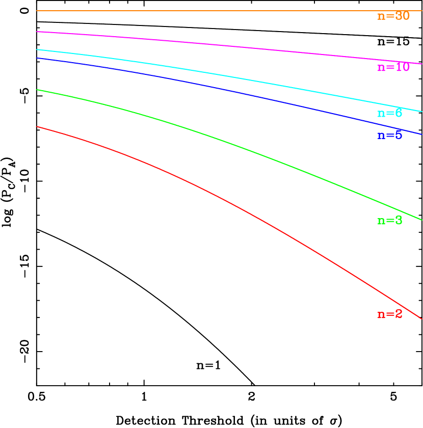
Figure 1: Ratios of the probabilities of false alarms, $P_{C}/P_{A}$, where $P_{A}$ is the probability for a sub-array where the signals from all the $N$ antennas are added incoherently, and $P_{C}$ is the joint probability for the case of $p$ sub-arrays each having $n=N/p$ antennas. Left panel: The ratios are plotted as a function of the number of antennas in a sub-array and for a detection threshold $T/\sigma$ = 3, for the total number of antennas $N$ = 3, 12, 21 and 30 respectively. Right panel: the same quantity $P_{C}/P_{A}$ is now plotted as a function of the threshold (in units of $\sigma$) for various sub-array combinations ($n$ = 30, 15, 10, 6, 5, 3, 2, 1) from the top to the bottom curve, for the case of $N~{}=~{}30$ (note that the curve for $n$ = 30 corresponds to the top horizontal line at log $P_{C}/P_{A}$ = 0) – see the text for more details.

Here we will describe ongoing efforts to equip the GMRT for transient exploration by (i) designing a software based system that will eventually function commensally with other observing programs, and (ii) undertaking pilot surveys that help demonstrate observational methodologies. This paper will focus on algorithms and methodologies, while the detailed implementation of a real-time processing pipeline and science results from pilot surveys are deferred to future papers. Apart from demonstrating the application of a “large-N, small-D” (LNSD) type instrument for transient explorations, these efforts will also enable new science with the GMRT. This is especially important given that the GMRT transients surveys will complement other similar efforts around the world in sky and frequency coverage.

This paper is organised as follows. In §2, we outline considerations that drive transient exploration strategies with interferometric instruments. In §3 we highlight unique advantages of the GMRT for this topic, and describe pilot surveys undertaken to aid the necessary technical development. Details of our transient detection pipeline are discussed in §4, and applications to real data are presented in §5. In §6 we discuss our event analysis pipeline and present examples illustrating important methodologies. In §7 we comment on possible future directions and in §8 we present our conclusions.

2 Interferometric Arrays for Transient Searches: Considerations and Strategies

In this section we discuss various considerations in searching for fast transient signals with interferometric instruments. We discuss various technical and sensitivity considerations that arise from the distributed nature of array elements, the role of propagation effects in signal detection and analysis, the importance of searching over a large parameter space and the use of long baselines to serve as spatial filters against RFI. While much of our discussion is presented within the context of the GMRT, we emphasise that these discussions are also applicable to other similar, particularly low-frequency, array instruments.

2.1 Technical and Sensitivity considerations

Array instruments can be used either in “incoherent array” (IA) or “phased array” (PA) modes for time-domain applications such as observing pulsars (Gupta et al., 2000), and in principle, similar strategies can be considered for the detection of fast transients. IA and PA correspond to modes which maximise the FoV and detection sensitivity (or the effective collecting area ${A_{\rm eff}}$), respectively. The IA mode is good for surveys, however it comes at the expense of a significant reduction in overall sensitivity. At the other extreme is a fully coherent array mode, where the signals from individual elements have to be combined to produce (many) phased-array beams within the primary beam in order to achieve the full FoV of the single element. This can be prohibitively expensive in terms of the real-time signal processing costs, as the number of beams goes as $(D/d)^{2}$, where $D$ is the physical extent of the array and $d$ is the size of the individual element or dish. For instance, application to just the central square (1 km $\times$ 1 km) of the GMRT requires the formation of $\sim$500 beams, whereas over $\sim 10^{5}$ beams will be required in order to realise the full FoV and sensitivity of the array. As a general rule, the use of phased-array beams for large surveys becomes less appealing as the filling factor of the array starts to fall-off.

An intermediate strategy that tries to optimize the trade-off between sensitivity and FoV and to maximise ${\rm A_{eff}\times FoV}$, while offering additional advantages for transient searches, is to use distinct sub-arrays with appropriately combined signals. These sub-arrays could be incoherent or coherent formations, for which we may then use statistical measures on sub-array detections to optimise the performance with respect to sensitivity, FoV, radio frequency interference (RFI) and excision of false positives etc. Here we describe the basis for such a scheme that has been implemented and tested using the GMRT array.

Our basic strategy is to generate a small number of incoherently summed sub-arrays and combine the candidate transient event detections from the sub-arrays in a manner that optimises the rejection of false positives via suitable coincidence filtering techniques. This will preserve the full FoV of a single element. To motivate this strategy, we consider the probability of false alarms in a transient detection scheme for various combinations of sub-arrays made from an array of N antennas. As described in detail in the Appendix, for an array of $N$ elements configured to make $p$ subarrays (with $n=N/p$ elements per sub-array), the joint false alarm probability is given by

$$P_{C}(>T)=\left[\frac{1}{2}\mbox{Erfc}\left(\sqrt{\frac{N}{2p}}\frac{T}{\sigma}\right)\right]^{p}~{},$$ (1)

where $T=r\,\sigma$ is the detection threshold and Erfc is the complementary error function (i.e. $r$ is the detection threshold in units of $\sigma$). As shown in the Appendix, $P_{C}$ can be significantly less than $P_{A}$, the false alarm probability for a single sub-array ($p=1,n=N$). This is illustrated in Fig. 1, which shows the ratio $P_{C}/P_{A}$ as a function of $n$ for different cases of $N$ and a fixed value of $r=3.0$ (left panel), and as a function of $r$, for different choices of $n$ and a fixed value of $N=30$ (right panel).

As evident from these figures, for an array of 30 antennas like the GMRT, the false detection rate can be improved by a few orders of magnitude by splitting the array into 4-5 sub-arrays of 6 to 7 antennas each. It is also clear that the improvements increase with a greater value of detection threshold. Since $r$ (as defined in the Appendix), is relative to $\sigma$ for the signal from a single antenna, realistic values (e. g. a 5-$\sigma$ threshold) for the different array combinations correspond to values of $r<5$ (e. g. $r\sim 1$ corresponds to a $\sim$5-$\sigma$ detection threshold for a single 30-antenna sub-array). For this range of $r$ values, improvements in the false detection rate by a factor of 10–100 can be obtained by splitting the array into 4-5 subarrays, while using the same detection threshold (say 5-$\sigma$).

Note that for the sub-array case, operating at the same detection threshold corresponds to a lower absolute sensitivity than the full array case. However, it should be possible to trade-off the false positive rate (while still keeping it below or comparable to that for the full array case) by reducing the threshold appropriately, thereby increasing the absolute sensitivity and bringing it closer to that of the full array. The sub-array case is expected to offer other advantages that accrue from rejection of false positives, such as discriminating against localised RFI; the effectiveness of this would depend on the physical extent of the full array, and how the antennas are grouped to form the sub-arrays.

Figure 2: The false alarm probability when sub-arrays with coincidence filters are used for the rejection of false positives. The resultant probability, $P_{C}$, is normalized to the probability for a single, 30-antenna incoherent array, $P_{A}$, and is shown as a function of the detection threshold $r$ and the number of antennas per sub-array $n$. Curves are drawn for ${\rm log}(P_{C}/P_{A})=-0.1,-1,-2,-4,-6,-8,-10,-12$ (top to bottom). These can be used as a guide to make the choice in terms of number of sub-arrays for a set threshold and desired level of rejection of false positives. For example, a 2$\sigma$ threshold ($r$=2) and $P_{C}/P_{A}$=100 require dividing the array into 10 sub-arrays.

Fig. 2 shows $P_{C}$ after normalisation to the probabilities of false alarms for a single incoherent array of all 30 antennas. Such plots may serve as useful guides to design an optimal observing strategy, e. g. to determine the number of sub-arrays required to realize a desired false positive rate for a set threshold, or to determine the threshold value that will be needed to achieve the desired level of rejection for a chosen number of sub-arrays.

The absolute sensitivity considerations are as follows. The sensitivity of a single element is characterised by its gain ($G_{a}$) and the system temperature (${\rm T_{sys}}$ ). For a sub-array of N antennas, a signal is detectable if its peak flux density (${\rm S_{pk}}$ ) exceeds some minimum flux density as determined by the radiometer equation:

$$S_{\rm pk,min}\,=\,K\,{\beta\,(T_{\rm rec}+T_{\rm sky})\over G_{\rm n}\,(\Delta\nu\,N_{\rm pol}\,W_{\rm p})^{1/2}}~{},$$ (2)

where $T_{\rm rec}$ and $T_{\rm sky}$ are the receiver and system temperatures, respectively ($T_{\rm sys}\approx T_{\rm rec}+T_{\rm sky}$ for most instruments), $G_{\rm n}$ is the net gain of the array in ${\rm K\,Jy^{-1}}$, $\Delta\nu$ is the recording bandwidth, $N_{\rm pol}$ is the number of polarisations, $W_{\rm p}$ is the matched filter width employed in transient searching, $\beta$ denotes the loss in signal-to-noise ratio (S/N) due to signal digitization, and the factor K is the detection threshold in units of rms flux density ($\sigma$).

For a 30-antenna sub-array on the GMRT, operating with a bandwidth of 32 MHz for a 5-$\sigma$ threshold, the achievable sensitivity for a survey would typically range from $\sim$1 Jy (at 610 MHz) for $W_{p}$=1 ms to $\sim$0.1 Jy for $W_{p}$=100 ms. As the single-antenna gain ($G_{a}$) and ${\rm T_{sys}}$ (when pointed to the cold sky) are comparable at 327 and 610 MHz, the nominal sensitivities are similar at both frequencies, though in practice the larger 327 MHz sky background (${\rm T_{sky}}$ ) will degrade the sensitivity.

When using sub-arrays (see e.g., Fig. 3 where the array is divided into five sub-arrays of six antennas each), however, $G_{\rm n}$ scales as $\sqrt{n}\,G_{\rm a}$. This leads to a worse sensitivity than that for a single $N$-element sub-array by a factor of $\sqrt{p}$. As mentioned above, some or all of this loss can be recovered by lowering the threshold by a corresponding factor, provided the resultant false positive rate remains better than that achievable for the default threshold with the single sub-array case.

2.2 Propagation effects

The role of plasma propagation effects in fast transient detection is discussed in detail by Cordes (2009) and Macquart (2011). These include dispersion, pulse broadening or scattering, and scintillation, and they are due to ionised interplanetary, interstellar and/or intergalactic media. While for most Galactic sources, the dominant contribution is from the interstellar medium (ISM), for sources at extragalactic or cosmological distances, there may also be significant contributions from the ISM of the host galaxy as well as from the intergalactic medium (IGM).

The differential dispersion delay, $\Delta t_{\rm dm}$ (in ms), across an observing bandwidth $\Delta\nu$ centred at an observing frequency $\nu$ (both in GHz) is given by $\Delta t_{\rm dm}\approx 8.3~{}{\rm DM}\,\Delta\nu\,\nu^{-3}$, where DM is the dispersion measure. For Galactic sources, DM can be up to several thousand ${\rm pc\ cm^{-3}}$ at large Galactic distances or toward the GC. Away from the Galactic plane, such large DMs can be expected for signals of extragalactic or cosmological origins.

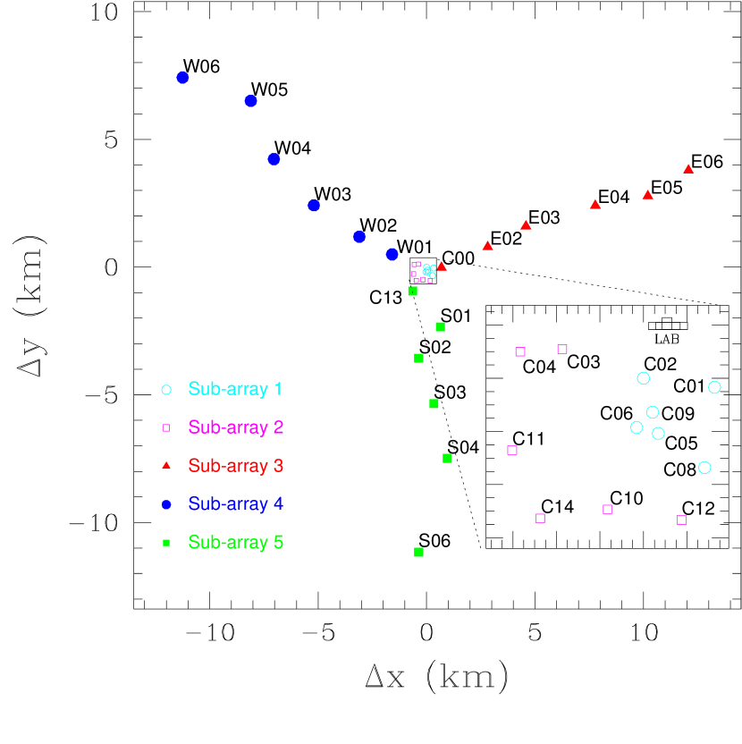
Figure 3: A map of the GMRT array indicating antenna locations across the east, west and south arms and in the central 1 km $\times$ 1 km region. The offsets ${\rm\Delta x}$ and ${\rm\Delta y}$ are relative to the antenna C02, which is at (${\rm\Delta x}$, ${\rm\Delta y}$) = (0, 0). The antennas can be grouped into multiple distinct sub-arrays of nearly equal sensitivities. The case for five sub-arrays is shown here: with three sub-arrays formed from antennas across the three arms, and the other two from antennas located in the central square. Such arrangements can yield high efficiencies in the identification and elimination of spurious events due to RFI.

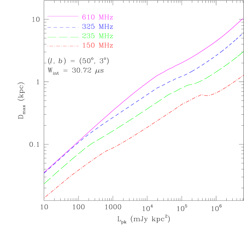
Figure 4: Plots of maximum distance to which transient detections are possible ($D_{\rm max}$ vs peak luminosity $L_{\rm pk}$), for the GMRT’s low frequency bands. $D_{\rm max}$ tends to vary linearly at low luminosities (i. e. smaller distances) when scatter broadening is negligible, and more slowly with increasing luminosity at large distances when scattering becomes prominent. While the nominal sensitivities are comparable for the GMRT at 325 and 610 MHz, scattering is important even at relatively lower distances at 325 MHz. The effect is more pronounced at lower frequencies, resulting in significantly lower values of $D_{\rm max}$ for $L_{\rm pk}$ and hence smaller search volumes for detectable signals.

Scattering (pulse broadening) leads to asymmetric pulse shapes with a stretched pulse tail. Measured pulse broadening times (${\rm\tau_{d}}$ ) scale steeply with the observing frequency; $\mbox{${\rm\tau_{d}}$\,}\propto\nu^{-3.9\pm 0.2}$ from observations (Bhat et al., 2004). Detection will thus become difficult when $\mbox{${\rm\tau_{d}}$\,}\gg\mbox{${W_{\rm int}}$\,}$, the intrinsic width of emission. For ${\rm\tau_{d}}$ $\scriptscriptstyle\stackrel{{\scriptstyle>}}{{\sim}}$ ${W_{\rm int}}$ , signal detection can still be critically influenced by the degree of scattering. While pulse broadening conserves the fluence (i. e. integrated flux), the smearing in time leads to smaller pulse amplitudes (i. e. lower peak flux densities), and hence lower signal-to-noise in the detection. Scattering can thus play an important role in defining optimal search strategies with low frequency arrays such as the MWA and LOFAR as well as the GMRT.

Both diffractive and refractive effects are important at low frequencies. Diffractive scintillation produces structure in both time and frequency, with the characteristic scales $\sim$100 s in time and $\sim$100 kHz in frequency for observations made at $\sim$300–600 MHz and for DMs $\scriptscriptstyle\stackrel{{\scriptstyle<}}{{\sim}}$ 50 ${\rm pc\ cm^{-3}}$ (e.g. Gupta et al., 1994; Bhat et al., 1998). As diffractive time scales are typically longer than $\sim$seconds, an apparent brightening or dimming of signals may arise in cases where diffractive bandwidth ($\nu_{d}$) is of the order of, or larger than, the recording bandwidth ($\nu_{d}\,\mbox{\raisebox{-0.43057pt}{$\scriptscriptstyle\stackrel{{\scriptstyle>}}{{\sim}}$\,}}\Delta\nu$). For distant sources, $\nu_{d}\ll\Delta\nu$, thus signal detection will be minimally affected. Refractive scintillation, on the other hand, leads to slow flux modulation on time scales of $\sim$days to weeks or longer (e.g. Gupta et al., 1993; Bhat et al., 1999).

Regardless of their impact on signal detectability, propagation effects can potentially serve as a useful discriminator from local RFI. While it may be possible for certain types of RFI to mimic one or more propagation effects, it is unlikely that non-astrophysical signals will emulate multiple effects in a manner consistent with models of astrophysical media.

2.3 Parameter space and search volume

In searching for short-duration radio transients, the two most basic search parameters are: (i) DM, and (ii) the duration of the signal. The latter is typically quantified as the effective pulse width, ${W_{\rm p}}$ . Here we briefly discuss the search parameter space, particularly in terms of limitations imposed by dispersion, scattering, detection sensitivity, and search volume.

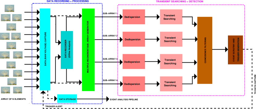
Figure 5: A diagrammatic representation of the GMRT transient detection pipeline. Raw voltage data from each array element are captured and made available to a processing pipeline. Multiple (incoherent) sub-array data streams are generated, and a transient search is performed on each data stream. The resulting events are assimilated through the event identification and coincidence filter algorithms to select the final candidates. For real-time implementation (dashed lines and arrows), this information is then used to generate triggers that will alert the raw data capture system to record relevant raw data segments for further detailed processing and scrutiny.

As discussed above, dispersion delays can be substantial, even at moderate DMs, for low radio frequencies; e. g. a pulse with $\mbox{${W_{\rm int}}$\,}=1$ ms and DM = 10 ${\rm pc\ cm^{-3}}$ will be smeared over $\sim$100 ms in observations with $\Delta\nu=32$ MHz centered at 300 MHz. While it is generally advisable to search out to very large DMs, in practice for searches within or near the Galactic plane, the maximum DM that can be effectively searched will likely be limited by pulse broadening. As the number of trial DMs are typically determined from analytical constraints that ensure minimal degradation of S/N due to DM errors, the DM spacings tend to be fairly small at low frequencies, thereby requiring a large number of trial DMs to span a given DM range. This can translate to significant processing costs for low frequency searches.

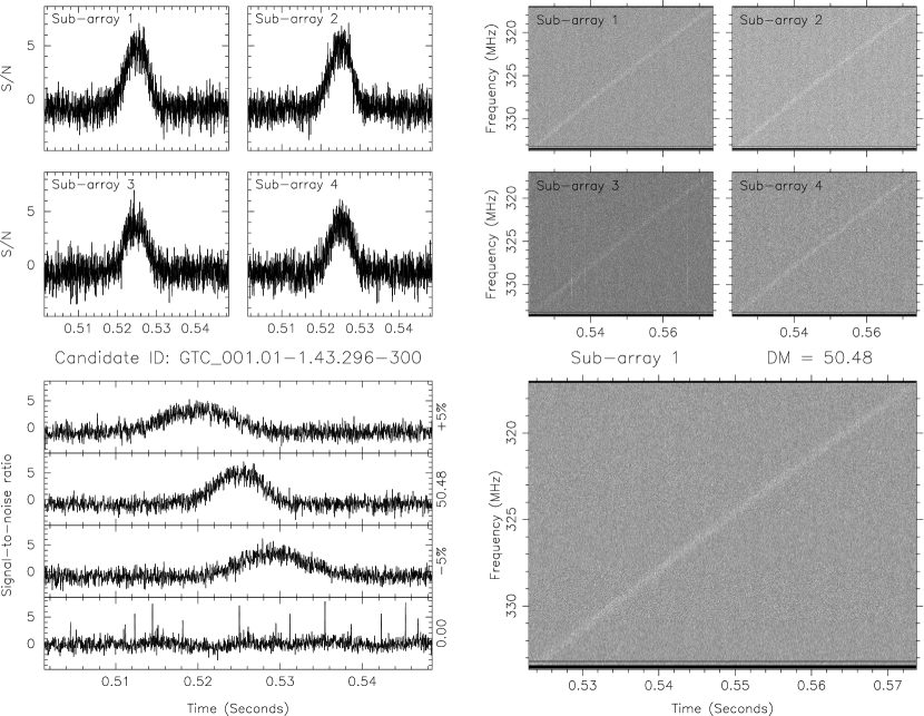
Figure 6: Example plots from the GMRT transient detection pipeline. A transient pulse was detected in the survey field GTC_001.01–1.43 (observations at 325 MHz, i. e. beam width $\approx$80^′). The pulsar PSR J1752$-$2806 is located at an offset of 42^′ from the phase center. The array was divided into four groups of roughly equal antennas, however the detection significance for the sub-arrays 2 and 3 (i. e. the south arm and the central square) were relatively lower, possibly due to the failure of some antennas to function at their nominally expected sensitivities. The top sub-panels show the de-dispersed time series (left) and frequency-time excerpts around the detected event (right). The bottom left sub-panels show the signal at two nearby DMs as well as at zero DM in addition to the candidate DM, while the bottom right panel is an enlarged version of the frequency-time plane excerpt around the signal. The detection of the signal in all four sub-arrays, its broad-band nature, dispersion sweep and a reduced S/N at nearby DMs and the absence of signal at DM=0 serve as multiple positive detection diagnostics.

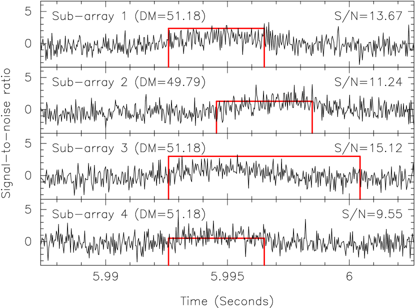
Figure 7: Another example detection from the GMRT transient pipeline, where the noise fluctuations lead to a transient pulse being detected at slightly different DMs and pulse widths in addition to different peak S/Ns across different sub-arrays. The true DM of the signal (i. e. a pulse from PSR J1752$-$2806 at $\sim 71^{\prime}$ offset from the phase centre) is closer to the DM value reported by the sub-array 2, in which the pulse was detected at a slightly reduced S/N (by $\sim 10\%$) at DM=51.18 ${\rm pc\ cm^{-3}}$ (i. e. the best DM as reported by other three sub-arrays). The widths and heights of the rectangle (red) boxes are proportional to the effective widths and peak S/Ns as found by the processing pipelines.

The vast spread in the duration of known transient phenomena make a compelling case to search in time duration over as wide a range as possible. In practice, the shortest time scale that can be effectively searched is limited to the sampling interval achievable with the recording instrument ($dt$); any signals of $\mbox{${W_{\rm int}}$\,}\mbox{\raisebox{-0.43057pt}{$\scriptscriptstyle\stackrel{{\scriptstyle<}}{{\sim}}$\,}}dt$ will thus be instrumentally broadened to $dt$. However, at low frequency, pulse broadening of astrophysical origin will likely exceed instrumental broadening, even at moderate DMs. At large DMs however, pulse broadening will limit the achievable (effective) time resolution, and it will be difficult to detect heavily scattered pulses owing to S/N degradation from broadening. The longest time durations that can be searched will therefore be dictated by pulse broadening.

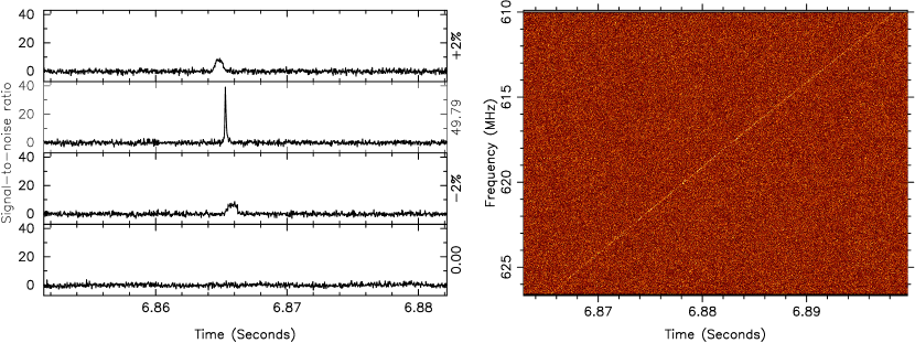
Figure 8: Example plots from the GMRT transient detection pipeline – the array was configured into seven different sub-arrays, each comprising a single antenna, thus providing a powerful coincidence filter against spurious events of RFI origin. Data were collected by emulating a ‘survey mode’, by scanning the sky region around the Crab pulsar at 0.5 ${\rm deg~{}min^{-1}}$. A bright giant pulse was detected as a ‘transient’ when the pulsar was within the telescope beam (half power beam width $\sim$0.5^∘). The pulse is very narrow ($\approx$50 $\mu$s), approximately twice the sampling resolution (30 $\mu$s) and so is seen as a thin strip on the waterfall plot. The signal peaks at DM = 56.74 ${\rm pc\ cm^{-3}}$ , with a sharp decline in S/N even at small departures from the true DM; for instance, ${\rm\Delta DM/DM\approx 0.02}$ results in a S/N loss of almost a factor of four, exemplifying the need for very short DM spacings and high time and frequency resolutions for transient searches at low radio frequencies.

Propagation effects may also significantly influence the maximum distance to which a detection is possible, $D_{\rm max}$, and therefore the search volume, given by $V_{\max}=(1/3)\Omega_{\rm s}D_{\rm max}^{3}$, where $\Omega_{\rm s}$ is the FoV. As $D_{\rm max}$ scales as $S_{\rm pk,min}^{-1/2}$, the prominent low-frequency effect is pulse broadening. The resultant amplitude degradation ($S_{\rm pk}\propto\tau_{d}^{-1/2}$) leads to a lower $D_{\rm max}$ and consequently a smaller search volume. A detailed treatment of this effect and relevant survey metrics are given by Cordes (2009), who considers different possible survey strategies, both for fast and slow transient searches with the SKA. Following the formalism presented there, useful plots can be made of $D_{\rm max}$ vs $L_{pk}$ (where $L_{pk}=S_{\rm pk}\,D^{2}$ is the peak luminosity) for a given choice of search parameters. As an illustration, Fig. 4 shows such sensitivity plots for different GMRT frequencies, for one specific line of sight within our pilot survey region ($l$=50^∘, $b$=3^∘). Here we account for various propagation effects, instrumental broadening, and the increase in sensitivity from using matched filtering. Reduced sensitivities (in the lower $L_{pk}$ range) at 150 and 235 MHz are due to the relatively larger sky backgrounds at these frequencies. As evident from these plots, $D_{\rm max}$ is reduced at higher $L_{pk}$ (i. e. larger distances for a given $S_{\rm pk}$), resulting in departures from linear trends compared to the lower $L_{pk}$ range. This effect is obviously direction dependent, thus making detection rates a strong function of sky position and frequency (e.g., Macquart, 2011). Such considerations may be used to optimize strategies for maximal survey yields.

2.4 Radio frequency interference

Impulsive and narrow-band RFI can be a major impediment in the detection of fast transients, increasing the number of false positives and raising the system noise. The issue of a false positive increase is particularly poignant for real-time detection schemes. With the ever-increasing number of (especially potentially astrophysically mimicking) RFI sources and the advent of wide-bandwidth observing systems, it is becoming imperative to develop mitigation strategies for a wide variety of RFI sources and signals.

Significant resilience to RFI can be developed through the use of appropriate instrumentation and online identification and excision schemes. Systems that use multi-bit recording can have significant dynamic range advantage over the traditional one- or two-bit recorders used in most systems. Prominent among prospective online mitigation schemes are those which employ median absolute deviation or spatial filtering (e.g. Roy et al., 2010; Kocz et al., 2010) and spectral kurtosis filtering methods (Nita & Gary, 2010). Effectiveness of a given strategy will depend on the instrument as well as the RFI environment.

Even with online schemes, however, a large number of false positives may pass through the processing pipeline, requiring post-detection mitigation schemes so that the number of candidate events that require human scrutiny can be reduced to a manageable level. This is especially critical for systems that need to function in a commensal mode. The long baselines of array instruments provide excellent capabilities here, enabling coincidence checks to allow identification and elimination of a large fraction of spurious events that are not common to all array elements. As outlined in §2.1, this forms the key strategy for our transient detection scheme for the GMRT. Coincidence filtering provides a simple but powerful strategy.

Instruments with interferometric capabilities offer yet another powerful means of discriminating against RFI-generated transient events. The signatures of real signals are likely to be distinctly different in the image plane in comparison to those due to RFI. As such, by their very nature, short-duration transients may be originating from sources that are necessarily compact and hence will likely be seen as point sources in the image plane, provided an image can be made at sufficiently high time resolution (e.g., Law & Bower, 2012). On the other hand, RFI bursts may yield various kinds of artifacts in the image plane, and are less likely to mimic the characteristics of point sources. Therefore by incorporating snap-shot imaging of candidate events among the event analysis strategies, further discrimination can be achieved against RFI sources.

3 The GMRT as a test bed instrument

The GMRT has a number of inherent design features which can be exploited for developing and demonstrating useful observing strategies for time domain science applications with next-generation instruments. In addition to those previously noted, the combination of moderate-sized paraboloids and operation at low frequencies mean relatively large fields-of-view, e.g. $\sim$6 ${\rm deg^{2}}$ at 150 MHz, $\sim$1.5 ${\rm deg^{2}}$ at 325 MHz. These, along with the capabilities of its new software backend (Roy et al., 2010), in particular its ability to capture raw voltage data from all 30 array elements and make them available to software-based processing systems and pipelines, are promising for a variety of exploratory development.

3.1 The GMRT software backend

The recently developed GMRT software backend (GSB), built using mainly commercial, off-the-shelf (COTS) components, is a fully real-time 32 antennas, 32 MHz, dual-polarization backend. The basic requirements for the GSB are to support two main modes of operation : (i) a real-time correlator and beamformer for an array of 32 dual polarized signals with a maximum bandwidth of 32 MHz, (ii) a base-band recorder where raw voltage signals from all the antennas can be recorded to disks, accompanied by off-line correlation and beamforming. Further details on design and implementation are described in Roy et al. (2010).

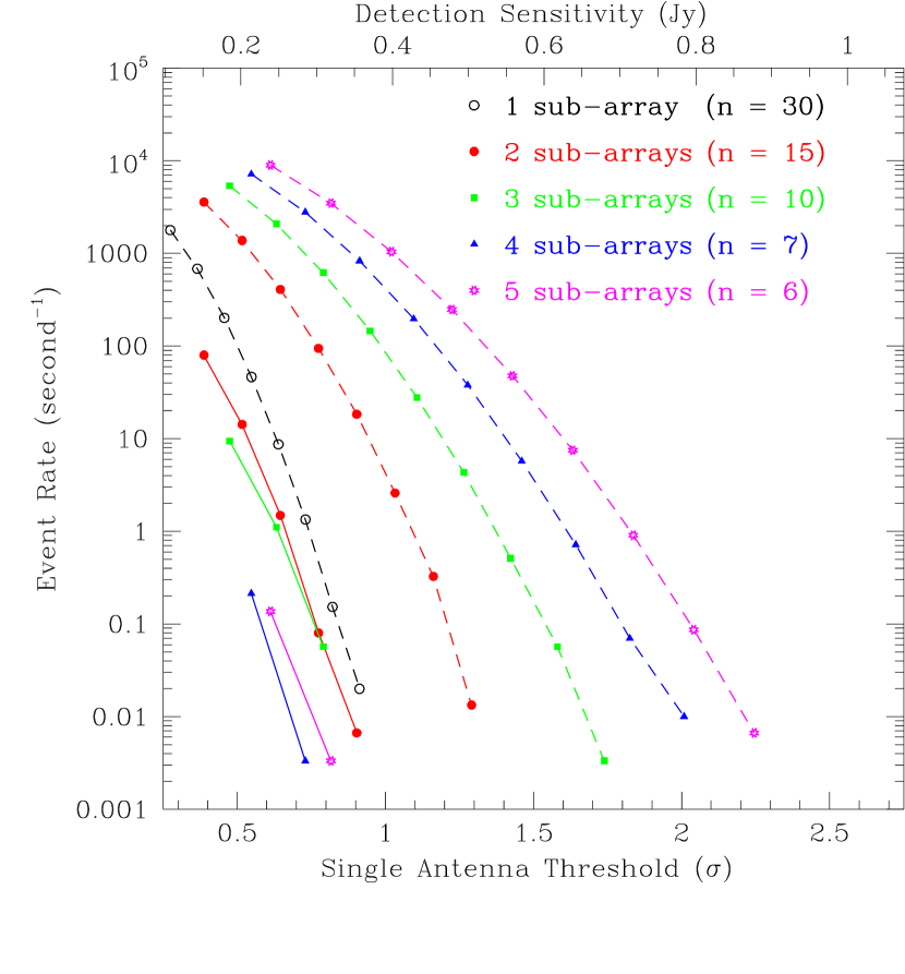
Figure 9: Event rate vs. detection threshold for different sub-array combinations possible with the GMRT array, for a representative data set to characterize false positives due to signal statistics. For each combination, a pair of curves are shown, where the top and bottom (dashed and solid) ones correspond to the event rates at the pre- and post-coincidence filtering stage. The pre-coincidence (dashed) curves denote the aggregate event rates from multiple different sub-arrays (i. e. the sum total of the event rates) for a given combination. Detection sensitivity is a strong function of the number of antennas included in a given sub-array, while the coincidence power increases with the number of sub-arrays.

3.2 Transient exploration with the GMRT

For transient exploration, our eventual goal is to develop and implement a system that will generate and process multiple incoherent array data streams in real-time for detecting transient candidate signals, and trigger the data recording system to extract and store relevant raw data segments for detailed offline investigations. Given the complexity of the problem, we adopt a two-phase strategy: the first phase involves conducting some pilot surveys and the development of a processing pipeline that operates on recorded raw voltage data. The outcomes from these are then used to finalise the design considerations for a real-time transient detection system. Among the most powerful features of such an approach are:

• exploitation of long baselines for powerful discrimination between signals of RFI origin and those of celestial origin via effective coincidence filtering and cross-checks between multiple independent data streams.

• event localisation possible via high-resolution imaging (5-10^") and/or full beam synthesis across the FoV, both for important integrity checks as well as for facilitating high-frequency and multi-wavelength follow-ups with other instruments.

• the ability to form sensitive phased-array beams toward targets of interest and record baseband data so as to enable high time resolution studies of signal characteristics including coherent dedispersion and polarimetry.

The modest recording bandwidth (maximum 32 MHz) of the current GMRT makes this a feasible exercise in terms of the related data rates and processing requirements. Even though the GMRT’s FoV is relatively small in comparison to those of SKA pathfinder instruments such as ASKAP or MeerKAT, the gain of a single antenna of the GMRT is almost 10 x larger than that of a single ($d\sim 12$ m) element of these next-generation arrays. Thus, with an aggregate effective collecting area of $\sim$ 3% SKA, the GMRT makes a highly sensitive instrument for conducting useful science demonstrations.

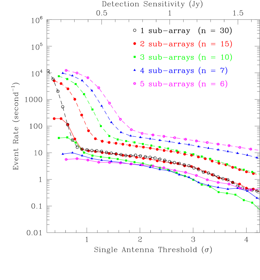
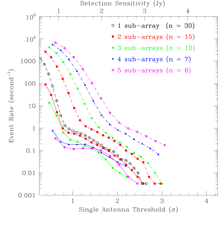
Figure 10: Plots similar to Fig. 9, for a field encompassing a known pulsar. The pulsar (PSR J1752$-$2806) is located near the edge of the $\approx$ 1.5 ${\rm deg^{2}}$ FoV (i. e. $\approx 70^{\prime}$ offset from the phase center). Left: processing at the pulsar DM and over the full recorder bandwidth ($\Delta\nu$=16.66 MHz); right: processing over a narrow bandwidth ($\Delta\nu/8$) to emulate weaker pulses. The detection sensitivity in Jy (top label) is based on nominal gain and system temperature for the GMRT at 325 MHz.

3.3 A pilot transient survey with the GMRT

In order to aid the related technical development and demonstrate the scientific credibility of transient exploration strategies, we conducted a pilot survey for short-duration transients with the GMRT, covering a small area of the sky ($-10^{\circ}\leq l\leq 50^{\circ}$ and $|b|\leq 3^{\circ}$) with fairly short dwell times (5 minutes per pointing). The data were collected in a specially designed observing mode where raw voltage streams from all 30 antennas were recorded on to the disks. This survey was conducted at 325 and 610 MHz, where the GMRT offers its highest sensitivity, due to the large gains (G$\sim$10 ${\rm K\,Jy^{-1}}$ for the full array) and relatively low system temperatures (${\rm T_{sys}}$ $\sim$ 100 K) at these frequencies. The region within $1^{\circ}$ of the plane was surveyed at 610 MHz and the areas above and below this at 325 MHz. This choice was based on two main considerations: (1) to alleviate severe scattering at low frequencies, in particular very close to the plane and toward the Galactic centre; (2) to optimise the survey speed: ${\rm 18~{}deg^{2}~{}per~{}hr}$ at 325 MHz vs ${\rm 5~{}deg^{2}~{}per~{}hr}$ at 610 MHz, so that the survey is completed within a modest amount of telescope time. The specific sky region was chosen because of its significant overlap with that of the Parkes Multibeam survey (thereby allowing immediate high frequency checks of any promising candidates), and also because it is the sky region where the density of known pulsars and rotating transient objects is the largest. The relatively short dwell times mean that the survey is primarily sensitive to sources with fairly high event rates (10 ${\rm hr^{-1}}$ or more), such as giant-pulse emitters and rotating radio transients.

In addition to the above pilot surveys, we also conducted observations in a number of exploratory modes. These include modes in which the array was sub-divided into multiple different groups (i.e. sub-arrays), with all configured to make pointed observations of a single selected target (such as the Crab pulsar), as well as modes in which different sub-arrays were configured to point to different targets of choice (i.e. a variance of the Fly’s Eye observing mode). These observations were made at a frequency of 610 MHz.

Given our primary technical objective of developing a transient detection system and the required methodologies, it was imperative to record this survey data in the “raw dump” mode of the GMRT software backend. This exploratory mode allows recording raw voltages from all 30 elements of the array, in two polarizations, with either 2- or 4-bit digitization. The aggregate data rate was approximately 1 ${\rm GB\,s^{-1}}$ or 3.6 ${\rm TB\,hr^{-1}}$ (from 30 $\times$ 2 signal paths). For the survey parameters outlined above, this amounts to 42 hr of on-sky time, translating into a total data volume of 151 TB. These data were transported to the Swinburne supercomputing facility where all processing and analyses were carried out. Transient searches spanned up to 1000 ${\rm pc\ cm^{-3}}$ in DM (in 1000 DM steps) and a maximum time scale of $\approx$500 ms. More details on the processing and results will be reported in a future publication.

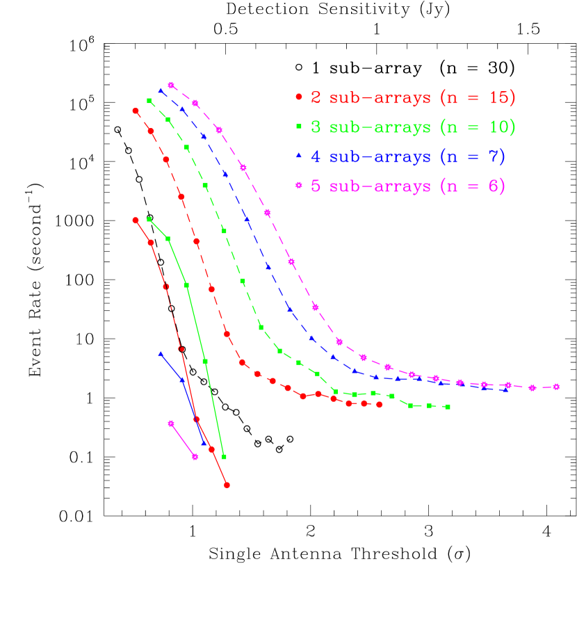
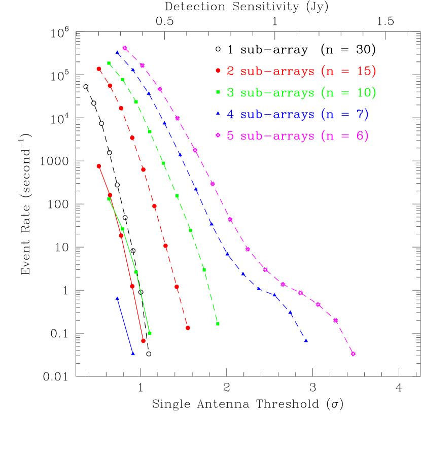
Figure 11: Plots similar to Fig. 9, where the chosen fields correspond to “blank skies” (i. e. fields that contain no detectable known pulsars or rotating radio transients) and during the conditions when the RFI-generated false positives were numerous. The left panel is the results for the survey field GTC_352.17+1.27 when RFI was comparatively severe (in terms of the RFI-generated events), and the right panel shows the results for another field GTC_002.25+1.17 when RFI was relatively modest.

4 Transient detection pipeline

In this section we outline a transient detection pipeline that we developed for offline analysis of the data from the pilot survey with the GMRT. We delve into various steps involved as we proceed from raw voltage data to the detection and final scrutiny of candidate events. The data from our pilot survey runs were used as test beds for developing the related software. In this paper we focus primarily on methodology and algorithms, with the implementation details to be reported in a separate paper.

The basic idea involves generating multiple incoherent sub-array beams and using coincidence filter schemes for the rejection of false positives and RFI. The array layout of the GMRT and a possible scheme for sub-dividing into multiple distinct groups (sub-arrays) is shown in Fig. 3. The block diagram of the processing pipeline is depicted in Fig. 5. Even though our beamformer software has been heavily optimized for a specific architecture (a constraint that arises from the GSB design considerations; see Roy et al. (2010)), the general scheme may also be applicable to other array instruments such as ASKAP or MeerKAT.

4.1 Raw data capture from array elements

As we demonstrate in later sections, access to raw voltage data from individual array elements offers a great deal of flexibility in terms of planning and conducting efficient transient searches with multi-element interferometric instruments. The raw voltage data can be easily interfaced to an incoherent beam former that offers the choice of the number of sub-arrays as well as the number of elements per sub-array. The sensitivity and other requirements of transient searching outlined in § 2.1 can thus be met with minimal constraints. Moreover, such flexibility can also be exploited to adapt to the changes in the RFI environment across the array.

The baseband recorder mode of the GSB can be configured for either 16 or 32 MHz bandwidth, with 4 or 2 bit digitisation respectively, so that the aggregate data rate is limited to 1 ${\rm GB\,s^{-1}}$ or 3.6 ${\rm TB\,hr^{-1}}$ (again a constraint imposed by the GSB design considerations). The recording cluster used in the current system comprises 16 nodes, each with 4 TB of data storage, thereby providing a total data storage capacity of 64 TB, i. e. a capability that can cater up to 18 hr of continuous baseband recording. There are four 1 TB disks connected to each node, and data from each antenna are streamed into separate disks. Each recorded data buffer is accompanied with a timestamp derived from the NTP server.

Online RFI detection and excision is an important consideration for transient detection with the GMRT. Of the prospective schemes described in § 2.4, filtering that relies on median absolute deviation is the only technique that has been tested on the GMRT data (e.g. Roy et al., 2010). It is our aim to further explore the efficacies of this as well as other methods in the detection of short-duration transients, and converge on a possible implementation scheme for the real-time version of our pipeline. We have incorporated some rudimentary data quality checks in our current processing pipeline. These include basic sanity checks of each and every data stream for any instrumental failures or malfunctioning and then using this information to suitably reconfigure relevant sub-arrays as well as the related coincidence parameters.

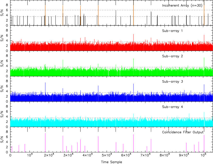
Figure 12: An illustrative example to highlight the power of multiple sub-arrays and coincidence filter for the detection of real astronomical transient events whose peak amplitudes may be well below typically used 5-6$\sigma$ thresholds. Data from a field encompassing a known pulsar (but located at a large offset from the phase center) are processed over a small fraction of the recording bandwidth ($\Delta\nu/8$) to mimic such a scenario. The top panel shows the raw time series (at the original time resolution of 30.72 $\mu$s), followed by the detections from a single incoherent sum of all 30 antennas for two set thresholds of 6$\sigma$ and 3.5$\sigma$ (i.e. second panel from the top); the four panels that follow (from third to sixth) show the detections (at a much lower 1.8$\sigma$) from individual sub-arrays when the array is sub-divided into four groups. The bottom panel is the output from the coincidence filter. The large tics in the second and bottom panels are the reference markers for the expected locations of pulses. Of the 11 pulses within this short data block (6 s), all but the faintest pulse have been successfully detected.

4.2 Formation of multiple incoherent beams

The rationale for dividing the array into multiple sub-arrays and opting for an incoherent addition of the intensities from telescopes in each sub-array is already detailed in § 2.1 (see also Fig. 3). The simplest implementation of this procedure involves combining the signals from different elements of the array after the required delay and broad-band fringe phase corrections and spectral de-composition. This is currently realised through a software system that operates on 2 $\times$ ${N_{\rm ant}}$ raw data streams from the data acquisition cluster and 2 $\times$ ${N_{\rm sub}}$ sets of antenna ”masks” (where ${N_{\rm sub}}$ is the number of sub-arrays), and performs the relevant signal additions in parallel. These multi-channel filterbank data streams, with a time resolution = 2 ${N_{\rm chan}}$ /${f_{\rm samp}}$ , where ${f_{\rm samp}}$ is the Nyquist sampling frequency and ${N_{\rm chan}}$ the number of spectral channels, are then converted to intensities and summed after application of the suitable antenna masks. These incoherently added intensity data are integrated (if needed) to achieve the desired time resolution. For example, for processing the data from pilot surveys, we have configured this incoherent beamformer to output data streams with 256 spectral channels across the 16 MHz bandwidth ($\Delta f$ = 62.5 kHz) at a time resolution of 30.72 $\mu$s.

Higher time resolution can only be achieved at the cost of a reduced spectral resolution. Searches at low frequencies inherently benefit from high resolutions in both time and frequency, and therefore this involves trade-offs in terms of the maximum DM that can be searched and the achievable time resolution. For example, a higher spectral resolution (i. e. 512-channel filter bank sampled at 61.44 $\mu$s) at 325 MHz will allow searching out to larger DMs while still not limiting the detectability of intrinsically narrow signals such as giant pulses, as they will be scatter broadened to $\sim$1 ms.

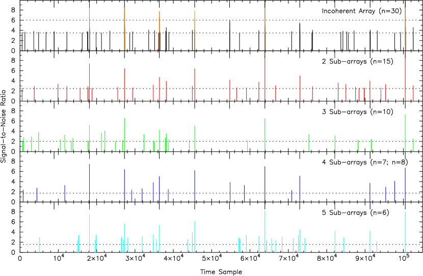
Figure 13: Another illustration to highlight the advantages of multiple sub-arrays and coincidence for transient detection. The data block is the same as that was shown in Fig. 12 but processed for different possible sub-array groupings. The top panel shows the raw data time series, followed by the detections from a full incoherent 30-antenna array (i.e. second panel from the top), while the bottom four panels correspond to cases where the number of sub-arrays range from 2 to 5. The large tics in the bottom five panels are the reference markers that indicate the expected locations of pulses. The dotted lines correspond to the detection thresholds for each of the different sub-array combinations. The detection efficiency progressively improves from 2 to 4 sub-arrays compared to a single incoherent sum, whereas 5 sub-arrays appears to be less than optimal choice. More quantitative analysis based on the processing of full data length (from this pointing) is summarized in Table 1.

4.3 Searching for transients

4.3.1 Dedispersion and Detection

Most traditional search algorithms for detecting fast transients operate on fast-sampled, multi-channel (filterbank) data and hence involve incoherent dedispersion followed by searching for transient events in the resultant time series. Dedispersion is performed over a large number of trial DMs (e.g. up to $\sim$1000 ${\rm pc\ cm^{-3}}$ ) using the standard direct dedispersion algorithm. This is the most computationally intensive part of our processing pipeline. As dispersion delays can be substantial at the GMRT’s frequencies (cf. § 2.2; $\mbox{${\Delta t_{\rm dm}}$\,}\propto\nu^{-3}$ for small $\Delta\nu$), a large number of trial DMs are required to span such a large DM range, even when observations are made over moderate bandwidths of 16-32 MHz.

Our current processing pipeline makes use of the dedispersion software that was developed for the ongoing high time resolution survey at Parkes (Keith et al., 2010; Burke-Spolaor et al., 2011). This software takes advantage of modern multi-core processors that allow multi-threaded software to achieve significant speed-ups in computation. While the Parkes survey decimates the data to two bits per sample, our processing pipeline is designed to operate on 16-bit data samples which provides a much higher dynamic range, and also ensures immunity against possible signal saturation from powerful RFI bursts. Following the convention in pulsar searches, spacings between DM values are determined by an analytic constraint on the signal-smearing due to incorrect trial DM. A GPU implementation of this dedispersion software has recently been developed (Barsdell et al., 2010) and is being integrated into the real-time version of our processing pipeline which will be described in a forthcoming paper.

Our approach of employing multiple sub-arrays for transient detection with the GMRT means that the dedispersion stage will result in $\mbox{${N_{\rm sub}}$\,}\times\mbox{${N_{\rm dm}}$\,}$ time series to search for, where ${N_{\rm dm}}$  is the total number of DM trials. As we demonstrate in later sections, four sub-arrays are optimal for transient detection with the GMRT. For our observing frequencies and recording bandwidth, ensuring a signal degradation (from dispersive smearing due to incorrect DM) of no more than 1% will necessitate $10^{3}$ time series for each sub-array.

Detection of transient events essentially involves the identification of data samples, or groups of samples, that are above a set threshold (e.g. 5$\sigma$) in the dedispersed time series. Matched filtering, as approximated through a range of box car widths, is the commonly employed detection technique (e.g. Cordes & McLaughlin, 2003). This simple, yet effective, methodology has been extensively used in a number of ongoing searches based at Parkes and Arecibo as well as other instruments around the world (e.g. Deneva et al., 2009; Burke-Spolaor et al., 2011; Bhat et al., 2011). Alternate techniques, such as those based on quadratic discriminants and other statistics, have also being explored and demonstrated to a certain extent (e.g. Thompson et al., 2011; Fridman, 2010; Spitler et al., 2012), though their efficacies as viable alternatives in large-scale transient searches have not yet been thoroughly tested. The present version of our pipeline therefore employs matched filtering as the primary detection algorithm.

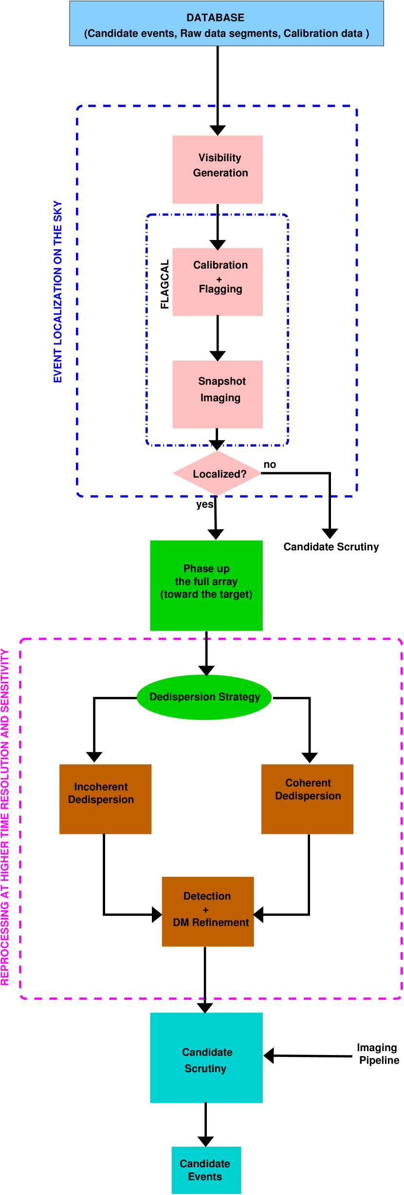
Figure 14: Diagrammatic representation of the event analysis pipeline for a detailed scrutiny of the candidate events that emerge from the GMRT transient detection pipeline. Depending on the characteristics of the candidate event, one or more analyses or scrutinies may be possible, e.g. processing of the raw data segments to generate the visibilities (for making a snapshot image of the FoV); forming a sensitive phased-array beam toward the target (to enable a high quality detection), followed by a suitable dispersion removal process and the signal detection. Final event scrutiny is then performed to arrive at a list of candidates for further follow-ups.

Matched filtering is approximated by progressive smoothing of time series data over a range of box car filters of widths $2^{n}$ samples, followed by application of threshold tests, each time recording the event amplitude, the time of occurrence and duration (e.g. Deneva et al., 2009; Burke-Spolaor et al., 2011). While relatively simple and easy to implement, this technique of matched filtering has some shortcomings; for instance, powerful RFI bursts that occur over relatively long durations (i. e. ${W_{\rm p}}$ $\gg$ $dt$) will be detected as an overwhelmingly large number of events. Furthermore, as the pulse templates have discrete widths of $2^{n}$ samples by design of the algorithm, this means reduced sensitivity to events whose widths are intermediate to those of the chosen box car filters. As discussed by Deneva et al. (2009) and Bhat et al. (2011), alternate methods, such as those based on time domain clustering along the lines of the friends-of-friends logic may help alleviate some of these demerits of matched filtering.

4.3.2 Initial scrutiny of detected events

An important consequence of the above described search strategy, which involves many trial DMs and box car widths, is that each single event will be detected as multiple events in the DM–time parameter space depending on the signal strength, duration and DM. In order to identify and associate multiple related events arising from a certain transient pulse, we employ algorithms along the lines of friends-of-friends logic that is very similar to those described in Burke-Spolaor et al. (2011). This essentially involves performing an association of events in time, DM and the matched filter width ${W_{\rm p}}$ , effectively identifying the groups of related events in the parameter space. In practice, this may be realized in two steps; first, for a given DM, association of related events is performed in time; specifically starting with the widest pulse and looking for pulses which overlap and, as each new pulse is associated, the search window is extended to include the net time range. The criterion here is that the peak of the second pulse overlaps with the full width of the first. A similar association is subsequently performed in DM, by effectively checking for contiguous events in DM and associating any events with the S/N characteristics that may follow likely astronomical signals (e.g. peaking at true DM and lower S/N with an increase in departure from the true DM). The procedure also accounts for possible time delays or advances expected due to the DM offset, thus ensuring that multiple real events of different DMs are detected as separate events, whereas multiple events due to a given RFI burst (often spanning the full DM range) are still detected as a single event. In the end, multiple points in the DM-time-${W_{\rm p}}$ parameter space which are related are counted as a single event.

4.4 Coincidence filtering and elimination of false positives

The main goal of coincidence filtering is the removal of false positives due to noise and RFI, thereby improving the efficiency to discriminate genuine signals of astronomical origin. In ideal conditions, when the signals are sufficiently strong to allow clear detections, this can be achieved with strict simultaneity checks in terms of the characteristics of the detected events. An example detection of this kind is shown in Fig. 6. However, real-world considerations necessitate a more flexible approach, especially when the detected signals are relatively weak (i. e. near the detection thresholds) and the sensitivity of the sub-arrays is not guaranteed to be identical. An example of these kind of effects can be seen in Fig. 12, which shows the detections from 4 sub-arrays of the GMRT, for a few successive pulses of a relatively weak pulsar where the detections are barely above the acceptable S/N threshold. As can be seen, sub-array 4 has a somewhat lower sensitivity than the other 3 sub-arrays, and even otherwise, the detectability of individual pulses does vary across the sub-arrays, presumably due to noise fluctuations. In such cases, it is possible that a given transient pulse may be detected at slightly different DMs, pulse widths (durations) or times of occurrence by different sub-arrays (an example for which is shown in Fig. 7), and an efficient recovery mechanism needs to take this into account.

In order to account for such effects and their potential impact on the detectability of genuine astrophysical signals, we have devised a somewhat flexible coincidence logic for the GMRT transient pipeline. Basically, each event is characterized by its basic properties such as the arrival time ($t$), duration ($w$), DM and the peak S/N. The events from different sub-arrays are cross-checked for coincidence criteria defined in terms of these parameters. Two events $E_{1}(t_{1},w_{1},DM_{1},s/n_{1})$ and $E_{2}(t_{2},w_{2},DM_{1},s/n_{2})$ from the sub-arrays 1 and 2 are treated to be coincident provided (i) overlap in their times of occurrence is within a set range, $T_{tol}$; (ii) the difference in DMs is within a set range, $DM_{tol}$; and (iii) the difference in the peak S/Ns is within a set range $S/N_{tol}$. That is, their characteristics need to be such that (i) $\delta DM\leq DM_{tol}$, (ii) $\delta(S/N)\leq(S/N)_{tol}$, (iii) $\Delta T/w_{1}\geq T_{tol}$ and (iv) $\Delta T/w_{2}\geq T_{tol}$, where $\delta DM$ and $\delta(S/N)$ are the fractional differences in the DMs and S/Ns, and $\Delta T$ is the overlap in the time ranges, as determined by the respective time ranges, $(t_{1},t_{1}+w_{1})$ and $(t_{2},t_{2}+w_{2})$ for the events $E_{1}$ and $E_{2}$. For coincidence between three or more sub-arrays, each event is checked against events from every other sub-arrays, beginning with the highest S/N event. As we illustrate in later sections, such a scheme is particularly important for the detection of weaker signals. Specifically, it increases the prospects of detecting real (weaker) signals, while limiting the number of false positives.

The parameters $T_{tol}$, $DM_{tol}$ and $S/N_{tol}$ thus determine the ”stringency” of the coincidence logic. For example, insisting for higher time overlaps (e.g. $T_{tol}$ $\scriptscriptstyle\stackrel{{\scriptstyle>}}{{\sim}}$ 50%) between the detected events imply a stringent coincidence logic, whereas allowing for smaller time overlaps (e.g. $T_{tol}$ $\scriptscriptstyle\stackrel{{\scriptstyle<}}{{\sim}}$ 20%) would result in a coincidence that is relatively more lenient. The parameters $DM_{tol}$ and $S/N_{tol}$ essentially help ensure that only those events of similar characteristics (in DM and brightness) have chances of passing through the coincidence filter. The choice of the above parameters also has implications in terms of the rates of false positives, since a more lenient coincidence logic means relatively higher rates of false positives. Similarly, a higher stringency in the coincidence logic may potentially result in filtering out real astronomical signals that are near the detection thresholds. Events that pass the set coincidence criteria are subjected to a further detailed scrutiny while those that fail are rejected from the analysis. While there may be various factors that influence optimal values of these parameters, RFI can also be expected to play a significant role, in particular for the GMRT given its location in a relatively RFI-prone environment.

On the basis of a preliminary analysis of our survey data (i. e. 130 fields covering a $\sim$200 ${\rm deg^{2}}$ of the sky) at 325 MHz, it appears that representative values may be $\sim$5–10% for $DM_{tol}$, and $\sim$50% for $(S/N)_{tol}$ and $T_{tol}$. Specifically, we note that these are derived particularly from the data on two specific survey fields (GTC_002.52–1.64 and GTC_001.01–1.43) that contained a known pulsar, but at relatively large offsets of 71’ and 42’ respectively from the beam phase center (i. e. near the edge and well outside the half power beam). These were processed for various possible combinations of the parameters, and the tolerance settings that resulted in maximal number of real pulse detections (and minimal number of false positives) were treated as optimal choices. These were subsequently verified using data from the pointings at the beginning of the survey observations (when the pulsar would be at the phase centre).

4.5 Examples of transient detections

Figure 6 shows an example candidate event detected in our survey observations (GTC_001.01–1.43) that contained a known pulsar at an offset of 1.2 deg from the phase center. This is from observations made at 325 MHz (i. e. a FoV $\approx$1.5 ${\rm deg^{2}}$ or a half power beam width $\sim 84^{\prime}$). These basic diagnostic plots illustrate a number of signal characteristics expected of astrophysical signals. For instance, the dedispersed time series and frequency-time plots (top panels) provide immediate assessments of coincidence of signal detection in multiple different sub-arrays. Other important signatures include a dispersion sweep in the time-frequency plane and the change in signal strength versus DM, which is shown as the dedispersed time series at the candidate DM as well as at two nearby DMs along with that at DM=0 (bottom panels). Our processing pipeline also records additional information such as signal strength vs. DM (for optimum ${W_{\rm p}}$ ) and signal strength vs Wp (for optimal DM). A basic scrutiny along these lines can be employed in order to arrive at a list of candidates that may require further detailed investigations.

Figure 15: Images of a single pulse from the pulsar J1752$-$2806. The left panel shows the “dirty” image, the sidelobe response of the interferometer can be clearly seen. The right panel shows the image after cleaning. The contour levels are logarithmically spaced between 20 and 270 mJy. The synthesized beam is shown in the top left corner and is $59^{{}^{\prime\prime}}\times 10^{{}^{\prime\prime}}$ in size. The flagging and calibration was done using the ${\rm FLAGCAL}$ pipeline, and the image was made using the AIPS task IMAGR.

Fig. 8 shows another example from our transient detection pipeline. These observations were made in a special mode where seven of the 30 antennas were pointed to the Crab pulsar, thus emulating 7 sub-arrays, each comprising a single antenna. This provides a powerful coincidence filter against spurious events of RFI origin. The data were collected in a ‘survey mode’, by making the telescopes scan the sky region around the Crab pulsar at a rate of 0.5 ${\rm deg~{}min^{-1}}$. A bright giant pulse was thus detected as a ‘transient’ when the pulsar was within the telescope beam (the half power beam width at 610 MHz is $\sim$0.5^∘). This example highlights the need to employ very short DM spacings as well as high time and frequency resolutions in order to retain sensitivity out to durations as short as tens of $\mu$s, which is possible with our transient pipeline.

5 Applications to Real Data

In § 2.1 we discussed the advantages of using multiple sub-arrays and coincidence for transient detection and its impact on the detection sensitivity to transient signals. In § 4.4 we delved into the details of practical implementation of our coincidence detection logic. In this section we present some examples to illustrate the effectiveness of such a scheme through its applications to real data obtained from our pilot surveys. Specifically, we highlight (i) the reduction of false positives for the cases of (a) pure noise, and (b) RFI contamination (§5.1), and (ii) the power of coincidence filtering in facilitating the detection of weaker astronomical signals (§5.2).

5.1 Reduction of false positives

The basic underlying concept here is that the vast majority of events generated due to noise fluctations and RFI signals will be uncorrelated between different sub-arrays. In order to investigate this, we compare the pre- and post-coincidence filtering event rates as a function of number of sub-arrays and detection threshold. We consider various possible combinations for the GMRT array, ranging from 2 to 5 sub-arrays, and process the data over a wide range of detection thresholds, down to $\sim$0.5$\sigma$ at the single antenna level. This analysis becomes fairly cumbersome given the complexity of the number of sub-array combinations and running the pipeline at the very low threshold values that we use. We therefore focus on some select case studies as described below.

5.1.1 Case study 1: A blank field in the absence of RFI

This is probably the simplest case, the results from which can be directly compared against the predictions based on the theoretical analysis presented in §2.1. To emulate an “absence of RFI”, we performed the related analysis on a data set that is virtually devoid of any noticeable RFI. To further reduce the effect of interference signals and keep matters simple, the data were processed at a single, large DM value (200 ${\rm pc\ cm^{-3}}$ ). Furthermore, the coincidence logic described earlier in § 4.4 was heavily simplified in order to match the assumptions made in the theoretical analysis (for instance, a uniform detection sensitivity across all different sub-arrays). Specifically, the tolerances in terms of DMs, arrival times and S/N ratios were set to zero, which implies the maximum possible stringency achievable with the coincidence logic.

The results from the analysis are shown in Fig. 9, where we plot both the pre- and post- coincidence filtering event rates for detection thresholds down to $\sim$0.5$\sigma$. The sub-array groupings of antennas have been chosen such that maximal resilience against localized RFI is achievable; e.g. in the case of four sub-arrays, 3 of them are formed from 7-8 antennas that are located along the east, west and south arms, whereas the fourth one is comprised of antennas from the central 1 km x 1 km area. The results for different sub-arrays have been scaled to equivalent single antenna thresholds by applying the theoretically expected scaling. The top panel denotes the thresholds in units of Jy, assuming nominal sensitivity parameters of the GMRT (cf. Eqn. 2). The 10 to 100 times improvement seen in the post-coincidence event rates compared to a single 30-antenna sub-array (i. e. the full GMRT array) is in rough agreement with the theoretical predictions (cf. Fig. 1, where the region of interest are the first 5 curves in the top left hand corner of the figure). There are however some discrepancies; for instance, the results for the 3 sub-array case are only marginally better compared to those for 2 sub-arrays. Moreover, little improvement is seen in going from 4 to 5 sub-arrays. These discrepancies may be due to some faint RFI signals that are common to different sub-arrays, or perhaps because of detection thresholds not scaling as theoretically expected in practice. Besides this, the results are in accordance with expectations from the theoretical analysis, thereby ratifying our basic principle for splitting the array into incoherent sub-arrays.

5.1.2 Case study 2: A blank field in the presence of RFI

The GMRT’s proximity to densely populated regions and operation at low frequencies pose major challenges in terms of corruption due to RFI. The main sources of RFI include power lines, transmitters, TV boosters and cell phone towers. Some of these are highlighted in (Paciga et al., 2011), which presents a detailed characterization of RFI sources seen in the GMRT’s $\sim$150 MHz band. A somewhat similar situation prevails at the other low frequency bands of the GMRT, even though it is true that most of the wideband, impulsive RFI sources have spectra that become weaker at higher frequencies. The preliminary processing of our pilot survey data suggests that at least some modest fraction of our survey data at 325 MHz is corrupted by RFI. The presence of multiple bright RFI sources, and short to moderate baselines of the array ($\sim$100 m to $\sim$25 km), lead to some interesting challenges in terms of gaining immunity against resultant false positives.

Different survey scans with varying degrees of RFI were identified and analyzed in order to investigate the improvement in terms of the pre- and post-coincidence event rates. One specific example is shown in Fig. 11. The combinations of 4 or 5 sub-arrays retain the discriminatory power in terms of immunity from RFI false positives, resulting in a significant improvement in terms of the rates of false positives compared to the reference case of a full incoherent array. However, the results for 2 and 3 sub-arrays are somewhat puzzling, particularly with regard to the improvement seen in going from 2 to 3 sub-arrays. In fact the 3 sub-array combination seems to be virtually ineffective when RFI gets severe (see left panel). This may suggest correlated RFI events between 3 sub-arrays; e.g. powerful RFI sources located near the central square region, the antennas from which are roughly evenly split between the 3 sub-arrays. While we have attempted to further investigate this puzzling observation by trialing different ways to form the sub-arrays (e.g. based on the proximity to the central electronics) and also by processing several different data sets, the results have not been quite conclusive. We therefore speculate this is likely to be an intrinsic feature of the GMRT array.

5.2 Detection of real astronomical signals

As outlined in § 2.1, an improved efficiency in terms of the rates of false positives can only be achieved at the cost of reduced sensitivities at individual sub-array levels. While our approach to divide the array into multiple groups of incoherent sums seems like a reasonable trade-off, the net result is reduced detection sensitivities, particularly to the detection of weaker signals. For instance, a 6$\sigma$ transient pulse from a single 30-antenna array will be detected as a 3$\sigma$ event when the array is sub-divided into four groups. An equally important aspect therefore is the efficiency that may be achievable in the detection of such weak (but real) astronomical signals. Lowering the detection thresholds to $\sim$2-3$\sigma$, in principle, should result in the detection of such signals, but this can be achieved only at the expense of a much larger number of false positives (mostly from signal statistics and perhaps some from RFI signals). As emphasised earlier, an underlying assumption is that the vast majority of these may be uncorrelated and therefore will be excised by coincidence filtering. In order to illustrate this, we conducted some specific analysis on suitably selected survey scans, the results from which are summarised below.

5.2.1 Case study: A field encompassing a known pulsar

The detection of genuine astrophysical signals is illustrated through an example survey field that contains a known pulsar (PSR J1752$-$2806) at an offset of 1.2^∘ from the phase center (i. e. $\approx 1.7\times$ the half power beam width at 325 MHz). The strength of the signal is such that, at the incoherent array output, the brightest pulses from the pulsar mimic intermittent transient signals, thus providing a very good test case. We processed these data at the pulsar’s DM (50.372 ${\rm pc\ cm^{-3}}$ ) and over the full recording bandwidth ($\Delta\nu$ = 16.66 MHz) as well as over a much reduced ($\Delta\nu/8\approx 2$ MHz) bandwidth; the latter was done in order to emulate even weaker pulses. The resultant plots of pre- and post- coincidence filtering event rates are shown in Fig. 10.

A quick inspection of these figures helps draw some useful conclusions. For example, in the full bandwidth case (left panel), all post-coincidence detection curves tend to merge near and above $\sim$1 $\sigma$, thus approaching the expected pulse rate $\approx$1.8 ${\rm s}^{-1}$. This may be interpreted as all genuine pulses that are bright enough (i.e. above the set detection thresholds) are detectable, thus providing crucial integrity checks of our processing pipeline. Secondly, for the reduced bandwidth case, where we emulate weaker pulses (i. e. S/N $\approx$ 3 times lower), while the event rates for 2 or 3 sub-arrays at lower thresholds ($\mbox{\raisebox{-0.43057pt}{$\scriptscriptstyle\stackrel{{\scriptstyle<}}{{\sim}}$\,}}1~{}\sigma$) are still dominated by false positives, a substantial improvement is seen on going to a larger number of sub-arrays. Overall this makes quite a compelling case to go for at least 4 sub-arrays. Furthermore, the improvement is only marginal on going from 4 to 5 sub-arrays, which suggests that 4 sub-arrays may be an optimal choice for transient detection with the GMRT.

5.2.2 Detection of weaker signals

Fig. 12 provides a useful illustration for the case of four sub-arrays. We have taken a short stretch of data from the above field that contains a known pulsar and presented a time domain analysis. Of the 11 real pulses (transient signals) present in this short data block, only 6 are detectable with the sensitivity of the 30-antenna incoherent array and a 6$\sigma$ detection threshold (top panel). In order to ensure the detection of all pulses, it turns out that the detection threshold needs to be lowered to 3.5$\sigma$. As seen from the figure, this also results in many more false positives along side. A 3.5$\sigma$ threshold scales down to $\sim$1.8$\sigma$ when the array is sub-divided into 4 distinct groups. Processing down to such low thresholds will obviously result in numerous false positives, as can be expected from signal statistics. However, as illustrated through this figure, virtually all of them are excised by the coincidence filtering, resulting in a very small number of false positives in the end. In fact, a quick glance of the figure (lower most panel) reveals that all but the faintest pulse is detectable, along side a relatively smaller number of false positives compared to that of the full 30-antenna array. This clearly illustrates that our basic theoretical ideas proposed in § 2.1 do work in practice in real data.

5.2.3 Optimal number of sub-arrays

Fig. 13 shows the net improvement achievable for different combinations of sub-arrays, i. e. from 2 to 5, compared to a single incoherent sum of all 30 antennas as reference (top panel), for the data set used in the analysis above. While there is a progressive improvement from 2 to 4 sub-arrays, the case for 5 sub-arrays is seen to be far less appealing compared to 4 sub-arrays. This inability of 5 sub-arrays to win over 4 sub-arrays may perhaps be due to possible departures in the detection sensitivity from the theoretically expected $\sqrt{\mbox{${n_{\rm ant}}$\,}}$ for incoherent sum, or because the algorithm becomes less effective due to a larger number of false positives at such very low (1.5$\sigma$) thresholds. In short, 4 sub-arrays seems to be an optimal strategy for transient detection with the GMRT.

In order to quantify the level of improvements as well as to obtain more meaningful statistics, we processed the full duration of the scan (300 seconds) and conducted similar analysis, the summary of which is shown in Table 1. The improvements are tabulated both in terms of detections of real pulses as well as the number of false positives. The data were split into two halves for this analysis, as often the number of detections will critically depend on the modulation of pulse amplitudes (due to intrinsic and/or scintillation effects). The first four columns of the table are self-explanatory; column 5 is the fraction of the number of real events found (normalized to the total number of real pulses that are present in the data), and the column 6 the ratio of the number of false positives compared to that of the full 30-antenna incoherent array. Overall, the results are consistent between the two data sets, particularly the improvement factor in terms of the number of false positives. It is also evident that of all the combinations, 4 sub-arrays yields the best improvement, which supports our finding from the example illustrated through Fig. 13.

6 Event analysis pipeline

Promising candidate events that emerge from our processing pipeline are subjected to detailed scrutinies, a basic scheme for which is shown in Fig. 14. Among the salient features are the integration of a calibration and imaging pipeline for potential on-sky localization of the event and the ability to phase up the full array toward the target position to enable a high-quality signal detection and confirmation. This necessitates keeping track of the calibrator observations and processing them routinely to solve for the complex gains of the array elements. For localization via imaging, the raw data segments of an event are first correlated to generate visibility data. Performing phase-coherent dedispersion prior to correlation can greatly increase the chances of localization, especially for short-duration signals at moderate or high DMs (e.g. giant pulses). In the event that a clear detection in imaging and accurate localization ($\sim$5-10”) is possible, a sensitive phased-array beam can be formed toward the target position to enable a high-quality signal detection and characterisation. Depending on the characteristics of the signal (e.g. time duration, temporal structure and DM), the phased-array data can then be processed for phase-coherent or incoherent dispersion removal followed by detection and subsequent analysis and further checks. As well as enabling crucial integrity checks of the detected events, such a powerful methodology offers the advantages of obtaining additional information – such as high time resolution studies, accurate DM estimation and localization of the target – for any genuine signals that may need further detailed follow-ups. Some of these possibilities are further elaborated and illustrated through suitable examples in the subsequent sections.

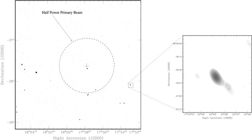
Figure 16: Image made from the correlated visibility data for the pointing GTC_002.52$-$1.64. The total time interval over which the visibilities are calculated is 0.8 seconds. The pulsar J1752$-$2806 was detected in this pointing by the transient search pipeline. The image shows a number of sources in the field, and the source corresponding to J1752$-$2806 is marked with a box. The image with the large field-of-view has a resolution of 36” x 20”. A zoomed-in image of the pulsar emission with a resolution of 16.5” x 8.5” is also shown. The contour levels in the zoomed in image start at 41 mJy and are in steps of 9 mJy. The position and flux measured from this image is RA = 17 52 58.746 $\pm$ 0.024, DEC = –28 06 36.09 $\pm$ 0.41 and $80\pm 9$ mJy.

6.1 Imaging pipeline

As described above, one of the major advantages of transient detection via interferometric arrays is the possibility of localisation of the source. This is most straightforwardly done by making an image of the transient. As described elsewhere in this paper, once a particular data stretch has been identified as containing a possible transient, the voltage data from each antenna for that corresponding time interval is saved. This data is then correlated (using essentially the same correlation routines as used in the real time system) to create a set of visibilities. The process of making an image from these visibilities is well understood (see e.g. Thompson et al. (2001)), and there exist several software packages aimed at doing this problem (e.g. AIPS, Miriad, CASA). The principal steps are (i) identifying and flagging out erroneous visibilities, e.g. those affected by radio frequency interference, which can be significant at most of the frequencies at which the GMRT operates, (ii) correcting for the complex gain (including the atmospheric/ionospheric gain) and (iii) imaging and deconvolution. The first two of these steps have been incorporated into a pipeline ${\rm FLAGCAL}$ (Prasad & Chengalur, 2012), while the imaging and deconvolution is currently done using one of the standard packages (AIPS in this instance)

6.1.1 Identification and flagging of corrupted visibilities

The most common type of strong RFI at the GMRT site has a small occupancy in the time-frequency space, i. e. is either limited in time, or in frequency, or in both. ${\rm FLAGCAL}$ uses this fact to identify corrupted visibilities. Essentially robust statistics (across time, frequency and baselines) of the visibilities are derived, and then outliers with respect to these statistics are identified and flagged out. Slow variations in the visibilities are accounted for by allowing for a (user definable) smoothing in the time frequency plane before computation of the statistics and identification of the outliers. In calibrator scans, one would expect that, in the absence of any corruption, the phase of the visibility would be nearly constant on the typical timescale of a calibration observation (i. e. of the order of a few minutes). This is also used to identify corrupted data. RFI often affects contiguous sets of channels and or time ranges, and hence two passes are made through the data, one of which identifies corrupted visibilities on the basis of the robust statistics, and the other that marginalises over the flagged data to identify frequency channels, baselines and/or antennas for which the data has been corrupted. The output of this stage of the pipeline is a set of visibilities in which all data identified as being corrupted has been flagged out. Since the determination of robust statistics is computationally intensive, ${\rm FLAGCAL}$ implements this using OpenMPI, resulting in significant speed ups in multi-core machines.

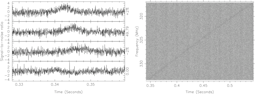
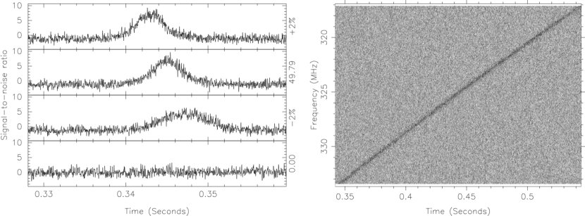
Figure 17: Example data illustrating the detection of a candidate signal and its subsequent confirmation and verification. The transient pulse (from a known pulsar that was within the FoV) was first detected at a relatively low significance ($\approx$5$\sigma$ at $\approx$0.25 ms resolution) and was treated as a candidate as it passed the set coincidence criteria. A sensitive phased array was then formed by phasing up all antennas with good calibration solutions toward the source position as determined by the on-sky imaging pipeline (see Fig. 16). The improved signal detection from this phased-array data is shown in the bottom panels. The peak signal-to-noise ratio improved by a factor of six, which is approximately 70% of the expected level of improvement given only 21 of the 30 antennas were phased up for final detection and verification.

6.1.2 Calibration

At any instant, an N-element interferometric array (i. e. one in which there are N unknown complex instrumental gains) measures $N(N-1)/2$ complex visibilities. This makes the problem of determining the antenna gains from observations of a calibrator source with known visibilities (e.g. a point source at the phase centre) over determined. Iterative schemes for determining the least squares solution for this problem have been described by e.g. Bhatnagar (2001). ${\rm FLAGCAL}$ implements this iterative scheme to determine the complex antenna gains. In general there are several kinds of calibrations that can be performed, viz. “flux calibration” for determining the absolute flux level; “bandpass calibration” for the spectral response; and “phase calibration” for the combination of the atmospheric and instrumental gains. ${\rm FLAGCAL}$ implements all of these calibrations and also interpolates the final corrections on to the target visibilities. It also allows interpolation of the flags from the calibration scans onto the target visibilities. This is useful in (the commonly encountered) situation where there is persistent RFI affecting some given spectral channels, antennas or baseline combinations.

6.1.3 Imaging and Deconvolution

The flagged and calibrated visibilities computed by ${\rm FLAGCAL}$ are written out as a FITS file. This allows easy processing using standard imaging packages. This stage of the processing can easily be automated. The GMRT array configuration has been designed to give a fairly good snapshot UV coverage at most declinations (see Swarup et al. (1991)) allowing for a good localisation of the source. As described above, this localisation is also important in determining that the transient emission that was detected indeed arises from the sky. In situations where there is sufficient signal-to-noise ratio, further confirmation of this comes from confirming that self calibration improves the signal-to-noise ratio of the image.

6.1.4 Case Study PSR J1752$-$2806

The pulsar J1752$-$2806 was targeted as part of the test observations on 2010 February 20. Calibration was done using the data from the source 1830$-$360 from the VLA catalog. The data was run through the ${\rm FLAGCAL}$ pipeline, and then imaged using the AIPS task IMAGR. The image was produced by excluding the edge channels, as well as some central channels which were badly affected by RFI and for which most of the data was flagged out. The final bandwidth used to make the image was $\sim 14.7$ MHz (i. e. $\approx$90% of the recording bandwidth), and the noise level in the image is $\sim 12$ mJy. The pulsar is clearly detected at a flux level of $\sim 220$ mJy. A strong confirmation that the emission arises from the sky (and is not some chance RFI) comes from the fact that self calibration significantly increased the peak flux of the source; specifically, the flux after one round of phase only self calibration is $\sim 280$ mJy. A similar confirmation comes from the fact that cleaning (which was done using the AIPS task IMAGR) substantially reduces the sidelobe levels. Fig. 15 shows the images produced before and after cleaning.

6.2 Application for event localization

We present another case study where a transient pulse was blindly detected in our search pipeline. The scenario is the same as that outlined in § 5.2.1, i.e. a survey field that contained a known pulsar but at a large offset of $\approx$71^′ from the phase centre. This large offset (1.7 $\times$ the nominal half power beam width) means a source location near the edge of the beam and as a result the pulsar will effectively be detected as an intermittently emitting transient source. The pulse was detected as a 5$\sigma$ event in the search pipeline and the signal characteristics (i.e. arrival time and DM) were then used to determine and extract the corresponding raw data segments from all 30 antennas. These data were then correlated to produce the visibilities which was subsequently imaged using the procedures described in § 6.1. Observations of 1830$-$360 that was recorded 36 minutes prior to the detection time of the transient pulse were used for calibrating the visibilities.

As a demonstration of our event localisation strategy, a snap-shot image was made of a $3^{\circ}\times 3^{\circ}$ region (nominal full beam width $\sim$1.4^∘) of the sky centred at the phase centre of the survey pointing (RA = 17h 57m 51.48s, DEC = $-$27d 36’ 00.0”). The pulsar was clearly detected in the image along with several other point sources in the field (see Fig. 16). The estimated pulsar position of RA = 17 52 58.746 $\pm$ 0.024, DEC = $-$28 06 36.09 $\pm$ 0.41 is within 2-3$\sigma$ of the catalog position and the measured flux $\sim$ $80\pm 9$ roughly agrees with the expected flux after scaling for the primary beam.

It is worth noting that even at this relatively bright flux level, there are a number of sources within the FoV. A cross check of the source positions in the image with the NVSS catalogue shows a good correspondence. The large number of “confusing” sources may partly be because the target field is close to the Galactic centre ($l=1.5^{\circ},~{}b=-1^{\circ}$). At fainter flux levels however, one would expect that there would be a number of background sources that would be present in the FoV. To distinguish between these and the transient source, we may apply either of the following two strategies: (i) make a fresh image centred on the time range during which the transient was the brightest – presumably the only source in this image whose flux will vary will be the transient; or, (ii) redo the transient search with a phased-array beam centred on each of the candidate sources – the signal-to-noise ratio would be the largest when the antennas are phased up toward the right position.

6.3 Phased array for improved signal detection and confirmation

In addition to producing incoherent array beams, the GSB beamformer can also generate coherent (phased) array beams. This involves performing suitable addition of pre-detected voltage samples from individual antennas. Coherent beam formation however requires calibrating out the antenna based phase offsets before the voltage samples can be added. These antenna based phases are solved using the recorded cross-correlations on a calibrator source near the target position, typically observed alongside the observations . As outlined in Roy et al. (2010), these phases are applied after the FFT stage, as an additional term in the fringe corrections.

As discussed in § 2.1, the incoherent array beam has the same field-of-view as the primary beam of a single antenna, but with an enhanced sensitivity of $\sqrt{N_{a}}$ times that of a single antenna, for an array of $N_{a}$ antennas. However, the coherent array beam is much narrower than that of a single antenna – similar to the synthesized beam obtained from the array of $N_{a}$ antennas, and therefore results in a sensitivity improvement of $N_{a}$ times than that of a single antenna. Hence by forming the coherent array beam towards the target source after phasing up the array, we expect $\sqrt{N_{a}}$ sensitivity improvement compared to the incoherent array.

As a demonstration of the follow-up strategy outlined above, we formed a phased-array beam at the position of the transient pulse in Fig. 16. The pulse was detected at a significance of 5$\sigma$ at a time resolution of $\approx$0.25 ms. The initial detection (at this resolution) and the final detection from processing the phased-array data are shown in Fig. 17 (top and bottom panels respectively). Data on the same calibrator source 1830–360 (i.e. recorded $\sim$30 min prior to the detection of the pulse) were used to solve for the antenna based phases required for phasing up the array. As seen from the figure there is 6 times improvement in the signal-to-noise ratio compared to the initial detection from the search pipeline. This is almost 70% of the theoretically expected improvement. A similar analysis was conducted on multiple other pulse detections and it suggests that up to $\sim$80% of the theoretically expected improvement may be achievable in practice. Even so, significant S/N improvements (as much as a factor 10) are still achievable in the final detections.

The discrepancy may be attributed to plausible calibration inaccuracies or some possible dephasing of arm antennas (due to ionospheric effects) given the 12.42^∘ separation between the pulsar and calibrator positions. In-beam calibration may help alleviate this in principle, however the GMRT’s FoV may often limit its prospects; e.g. while there are multiple point sources in Fig. 16, the brightest source has a flux of only $\sim$100 mJy, not good enough to derive reliable calibration solutions. However, this will no longer be a limitation for future wide-FoV instruments such as MWA, LOFAR and ASKAP that will contain multiple potential calibrator sources in any given field.

7 Future Work

While the analysis presented in this paper is largely based on our pilot survey data at 325 MHz, it is important to ascertain the efficacies and limitations of conducting transient searches at different frequencies of the GMRT. For instance, the RFI environment varies significantly between different frequencies and it will be very useful to investigate the effectiveness of snap-shot imaging for developing immunity against a variety of RFI-generated events. This will be the subject of a future publication. While the lower frequencies provide the basic advantage of comparatively larger fields-of-view (e.g. $\sim$6 ${\rm deg^{2}}$ at 150 MHz compared to $\sim$1.5 ${\rm deg^{2}}$ at 325 MHz), they also imply increased challenges in terms of having to deal with more severe RFI environments. The higher frequencies (e.g. 1400 MHz), on the other hand, while helping to extend the parameter space (i.e. searching out to larger DMs), may necessitate trading-off the achievable field of view ($\sim$0.1 ${\rm deg^{2}}$). We will conduct similar pilot surveys for all other frequencies GMRT to further optimise our processing pipelines and search algorithms.

Our eventual goal is a transient detection system for the GMRT that functions in a commensal mode with other observing programs. Having demonstrated the efficacies of multiple (incoherent) sub-arrays for initial detection and interferometric capabilities for on-sky localization, the next logical step is a real-time implementation of such a pipeline. The GPU-optimized dedispersion software developed at Swinburne (Barsdell et al., 2012) has been benchmarked for the GMRT frequencies and the current recording bandwidth of 32 MHz, and can handle up to $\sim$550 trial DMs (at both 325 and 610 MHz). The matched-filtering based detection is relatively inexpensive computation-wise and can easily be integrated, however recovering the loss in sensitivity (due to sub-arraying) through the use of very low detection thresholds (i.e. $\sim$2-3$\sigma$ compared to $\sim$5-6$\sigma$ typically used in transient searches) may require some optimisation of the downstream algorithms for event scrutiny.

We have outlined and demonstrated a specific approach for transient detection with interferometric arrays. While we advocate the use of multiple incoherent sub-arrays and coincidence checks as a promising strategy, there may be other possibilities that are worth exploring within the general context of next-generation instruments such as ASKAP, MeerKAT and the SKA, including, for example, the use of multiple sub-arrays to achieve larger fields-of-view (i.e. by pointing the sub-arrays in different regions of the sky). The improved sensitivity achievable through the use of wider-bandwidth recorders, and the constraints that may arise in terms of data rates and processing needs, are also among important aspects that need investigation. As the GMRT gets upgraded in the coming years through commissioning of its broad-band receivers and backends, new avenues will be opened up for undertaking such more promising, albeit more complex, science demonstrator projects relevant in the SKA-era.

8 Summary and Conclusions

While large single-dish instruments currently dominate time-domain science applications such as pulsars and fast transients, the future lies in the effective use of large-element interferometric arrays. The GMRT, with its modest number of elements and long baselines, makes a powerful platform for developing the necessary techniques and methodologies. In particular, its sub-array and interferometric capabilities can be well exploited for efficient detection of fast transients as well as for their accurate on-sky localisation.

Among the various considerations in the use of arrays for transient exploration is the trade-off between the field of view and absolute detection sensitivity. We have postulated the basic idea of generating a relatively small number of incoherently summed sub-arrays from the full array and then combining the results of detections of candidate transient events from each of these sub-arrays so as to optimise the rejection of false positives due to receiver noise and from RFI, using suitably devised coincidence filtering techniques. As we demonstrate through multiple examples and analysis, this enables reaching the sensitivity of the full phased array, while preserving the full FoV of the single antenna element. This approach is promising as it offers a dramatic improvement in terms of the prospects of detecting weaker signals. For example, a $\sim$2$\sigma$ detection from initial processing will eventualy be a $\sim$10$\sigma$ signal after phasing-up the full array, and hence will be both unambiguously verifiable in time series as well as localizable (on sky) at arc second accuracies.

The GMRT software backend allows raw voltage data from individual array elements to be recorded and made available for software-based pipelines. We have exploited this optional feature to develop and implement a transient detection pipeline for the GMRT. This includes a beamformer that operates on 2 $\times$ 30 raw voltage data streams to produce multiple incoherently summed sub-arrays, the data from which are then dedispersed and searched for transient events. The resultant events are scrutinised by the coincidence algorithms that take into account likely differences in the detection sensitivity between different sub-arrays that may result from either local RFI, or from one or more array elements performing at less than their nominal sensitivities. We have also explored the effectiveness of the algorithms as a function of the detection threshold as well as sub-arraying, and our analyses suggest that four sub-arrays make an optimal choice for transient detection with the GMRT.

Important future work includes undertaking pilot surveys at different frequencies of the GMRT in order to further optimise the strategies and algorithms for transient detection with arrays, and the development of a real-time version of the transient pipeline that can work in commensal mode.

The work described here, while demonstrating the applications of interferometric arrays for fast transient exploration – an important preparatory step for planned science with the SKA pathfinder instruments such as ASKAP and MeerKAT – also forms the first step to add new capabilities to the GMRT in the exciting arena of charting the transient sky at radio wavelengths.

Acknowledgements: This work is supported by the Australian Government under the Australia-India Strategic Research Fund grant ST020071 and by the Indian Government under the Department of Science and Technology grant DST/INT/AUS/Proj-14/2008. The Centre for All-sky Astrophysics is an Australian Research Council Centre for Excellence, funded by CE11E0090. N.D.R.B. is supported by a Curtin Research Fellowship and thanks Steven Tingay for support and encouragement extended to this project. We thank an anonymous referee for many useful comments that helped to improve the clarity of the paper. Data processing was carried out at Swinburne University’s Supercomputing Facility. We thank the staff of the GMRT for help with the observations. The GMRT is operated by the National Centre for Radio Astrophysics (NCRA) of the Tata Institute of Fundamental Research (TIFR), India.

Figure 18: The change in the computed PFA with threshold $r$ (in units of $\sigma$) for the case of one IA beam with $N$ antennas in the sub-array (solid line) and for the case of $N$ number of IA beams with one antenna in each sub-array (dashed line). The symbols mark the results from numerical simulations using Gaussian random noise.

9 Appendix: Probability of False Alarms for Sub-Array configurations

For the case where the random noise output signal of a radio telescope antenna follows a Gaussian distribution with zero mean and variance of $\sigma^{2}$, the probability of the signal level crossing a threshold $T$ is given by:

$$P(>T)=\int_{T}^{\infty}\frac{1}{\sqrt{2\pi}\sigma}\exp[-\frac{x^{2}}{2\sigma^{2}}]dx$$ (3)

or

$$P(>T)=\int_{T/\sqrt{2}\sigma}^{\infty}\frac{1}{\sqrt{\pi}}\exp[-y^{2}]dy=\frac{1}{2}{\rm Erfc}\left(\frac{T}{\sigma\sqrt{2}}\right)$$ (4)

where ${\rm Erfc}$ is the complimentary Error Function. We call $P(>T)$ the probability of false alarms (PFA), as these excursions would lead to false triggering of a transient detection pipeline where the detection threshold is set to $T~{}\sigma$.

For an array of $N$ such antennas, the signal can be combined in different ways. For a coherent phased array, the voltage signals from individual antennas are added in phase and then squared to get the total intensity, and then further integrated in time and frequency as required to get the final output. For an incoherent array, the intensity signals from individual antennas are added to get the total intensity signal and then integrated to the desired time and frequency resolution. The effective $\sigma$ decreases by a factor of $N$ or $\sqrt{N}$, for the coherent and incoherent array outputs, respectively (Gupta et al., 2000). Thus, for an incoherent array (IA) of $N$ antennas, the effective sigma is :

$$\sigma_{N}=\frac{\sigma}{\sqrt{N}}$$ (5)

where $\sigma^{2}$ is the variance for a single antenna.

In what follows we consider the following three cases of incoherent array :

(A) Single IA beam from a single sub-array of $N$ antennas:

For this case the probability of false alarms can be expressed as (from eqn A1 above):

$$P_{A}(>T)=\frac{1}{2}\mbox{Erfc}\left(r\sqrt{\frac{N}{2}}\right)$$ (6)

where $r~{}=~{}T/\sigma$ is the detection threshold in units of $\sigma$.

(B) $N$ IA beams from $N$ sub-arrays, each with one antenna:

In this case the false alarms due to noise statistics are independent events in each sub-array output, and if we use a coincidence filtering scheme where a false alarm is declared only if it is present simultaneously in all sub-array outputs, then the PFAs from all the IA beams get multiplied to give

$$P_{B}(>T)=\left[\frac{1}{2}\mbox{Erfc}\left(\frac{T}{\sigma\sqrt{2}}\right)\right]^{N}$$ (7)

(C) $p$ IA beams from $p$ sub-arrays, each with $n=N/p$ antennas:

The most general case is to have $p=N/n$ sub-arrays with each having $n$ antennas, for which the effective PFA is given by

$$P_{C}(>T)=\left[\frac{1}{2}\mbox{Erfc}\left(\frac{T}{\sigma}\sqrt{\frac{n}{2}}\right)\right]^{p}$$ (8)

Note that for $p=1,n=N,P_{C}=P_{A}$ and $p=N,n=1,P_{C}=P_{B}$. Also, it is easy to show that, for a given threshold $r={T}/{\sigma}$, $P_{B}<P_{C}<P_{A}$. This is illustrated in Fig. 18, which plots the PFA as a function of $r$ for the two cases $P_{B}$ and $P_{A}$, for the GMRT value of $N~{}=~{}30$. Results from simulation runs using random Gaussian noise (denoted by the symbols) are also overploted on the theoretically calculated curves. As can be seen, for small threshold values, log$P_{B}$ is less than log$P_{A}$ by a factor of 10 and this ratio increases with $r$ for values of $r~{}>~{}1$, reaching a value of around 26 for a threshold of 3.0. The curve for $P_{C}$ would lie in between the curves for $P_{A}$ and $P_{B}$.

From this, it is evident that there exists a possibility for trading off between PFA and $r$, for different choices of sub-arrays. For example, in order to have the same PFA for different combinations of sub-arrays, it is possible to work at lower thresholds for cases where the array is split into sub-arrays. This can offset the basic reduction in sensitivity that each sub-array suffers from (compared to the case of a single sub-array of $N$ antennas), while offering improved immunity against local interference signals that don’t pass the coincidence filtering test.

As an alternate illustration of the ideas, fig A2 shows the ratio of $P_{C}$ to $P_{B}$ (on a log scale) as a function of number of antennas in the sub-array, $n$, for different choices of total number of antennas, $N$, and for a fixed choice of $r~{}=~{}3.0$. Moving along any of these curves from $n~{}=~{}N$ to $n~{}=~{}1$ illustrates how the PFA reduces as more numbers of sub-arrays are used.

Thus, it is possible to reduce the probability of false alarms by using multiple sub-arrays, and this can be used to trade-off sensitivity (via different threshold values) vs false alarm rate to optimise the performance from the entire array.

Table 1: Coincidence filtering: event list summary

$N_{\rm sub}$	$r$	$N_{\rm real}$	$N_{\rm false}$	$f_{\rm real}$	$f_{\rm false}$
(1)	(2)	(3)	(4)	(5)	(6)
Data segment 1 (0 - 150 seconds)
1	3.5	62	1193	0.25	1
2	2.5	113	615	0.45	0.52
3	2.0	121	653	0.49	0.55
4	1.7	112	367	0.45	0.31
5	1.5	108	537	0.43	0.45
Data segment 2 (150 - 300 seconds)
1	3.5	92	1243	0.39	1
2	2.5	146	601	0.62	0.48
3	2.0	119	761	0.51	0.61
4	1.7	133	393	0.57	0.32
5	1.5	131	564	0.56	0.45

Note. — Results from a coincidence filtering analysis of the survey field GTC_002.52–1.64 where a known pulsar (PSR J1752$-$2806) was present at an offset of $\approx$1.2^∘ from the beam phase centre (i.e. outside the half power primary beam; see Fig. 16). Number of sub-arrays ($N_{\rm sub}$) varied from one to five, and the detection thresholds are scaled down assuming the theoretically expected $\sqrt{n}$, where $n$ is the number of antennas per sub-array; the number of real events and false positives ($N_{\rm real}$ and $N_{\rm false}$) are tabulated along with the corresponding fractions ($f_{\rm real}$ and $f_{\rm false}$).

References

- Barsdell et al. (2012) Barsdell, B. R., Bailes, M., Barnes, D. G., & Fluke, C. J. 2012, MNRAS, 422, 379
- Barsdell et al. (2010) Barsdell, B. R., Barnes, D. G., & Fluke, C. J. 2010, MNRAS, 408, 1936
- Bhat (2011) Bhat, N. D. R. 2011, Bulletin of the Astronomical Society of India, 39, 353
- Bhat et al. (2004) Bhat, N. D. R., Cordes, J. M., Camilo, F., Nice, D. J., & Lorimer, D. R. 2004, ApJ, 605, 759
- Bhat et al. (2005) Bhat, N. D. R., Cordes, J. M., Chatterjee, S., & Lazio, T. J. W. 2005, Radio Science, 40, 5
- Bhat et al. (2011) Bhat, N. D. R., Cordes, J. M., Cox, P. J., et al. 2011, ApJ, 732, 14
- Bhat et al. (1998) Bhat, N. D. R., Gupta, Y., & Rao, A. P. 1998, ApJ, 500, 262
- Bhat et al. (1999) Bhat, N. D. R., Rao, A. P., & Gupta, Y. 1999, ApJS, 121, 483
- Bhat et al. (2007) Bhat, N. D. R., Wayth, R. B., Knight, H. S., et al. 2007, ApJ, 665, 618
- Bhatnagar (2001) Bhatnagar, S. 2001, PhD Thesis, Pune University
- Booth et al. (2009) Booth, R. S., de Blok, W. J. G., Jonas, J. L., & Fanaroff, B. 2009, arXiv:0910.2935
- Bower et al. (2007) Bower, G. C., Saul, D., Bloom, J. S., Bolatto, A., Filippenko, A. V., Foley, R. J., & Perley, D. 2007, ApJ, 666, 346
- Burke-Spolaor et al. (2011) Burke-Spolaor, S., Bailes, M., Ekers, R., Macquart, J.-P., & Crawford, F., III 2011, ApJ, 727, 18
- Burke-Spolaor et al. (2011) Burke-Spolaor, S., Bailes, M., Johnston, S., et al. 2011, MNRAS, 416, 2465
- Camilo et al. (2006) Camilo, F., Ransom, S. M., Halpern, J. P., et al. 2006, Nature, 442, 892
- Chandra & Frail (2011) Chandra, P., & Frail, D. A. 2011, Bulletin of the Astronomical Society of India, 39, 451
- Coenen et al. (2012) Coenen, T., & The LOFAR Pulsar Working Group 2012, arXiv:1211.1885
- Colegate & Clarke (2011) Colegate, T. M., & Clarke, N. 2011, PASA, 28, 299
- Cordes (2009) Cordes, J.M., 2009, SKA Memo 97
- Cordes et al. (2004a) Cordes, J. M., Bhat, N. D. R., Hankins, T. H., McLaughlin, M. A., & Kern, J. 2004, ApJ, 612, 375
- Cordes et al. (2006) Cordes, J. M., Freire, P. C. C., Lorimer, D. R., et al. 2006, ApJ, 637, 446
- Cordes & Lazio (2002) Cordes, J. M., & Lazio, T. J. W. 2002, arXiv:astro-ph/0207156
- Cordes et al. (2004b) Cordes, J. M., Lazio, T. J. W., & McLaughlin, M. A. 2004, New Astronomy Review, 48, 1459
- Cordes & McLaughlin (2003) Cordes, J. M., & McLaughlin, M. A. 2003, ApJ, 596, 1142
- Deneva et al. (2009) Deneva, J. S., et al. 2009, ApJ, 703, 2259
- Fender & Bell (2011) Fender, R. P., & Bell, M. E. 2011, Bulletin of the Astronomical Society of India, 39, 315
- Fridman (2010) Fridman P. A., 2010, MNRAS, 409, 808
- Garrett et al. (2010) Garrett, M. A., Cordes, J. M., Deboer, D. R., Jonas, J. L., Rawlings, S., & Schilizzi, R. T. 2010, arXiv:1008.2871
- Gupta et al. (2000) Gupta, Y., Gothoskar, P., Joshi, B. C., et al. 2000, IAU Colloq. 177: Pulsar Astronomy - 2000 and Beyond, 202, 277
- Gupta et al. (1993) Gupta, Y., Rickett, B. J., & Coles, W. A. 1993, ApJ, 403, 183
- Gupta et al. (1994) Gupta, Y., Rickett, B. J., & Lyne, A. G. 1994, MNRAS, 269, 1035
- Hankins et al. (2003) Hankins, T. H., Kern, J. S., Weatherall, J. C., & Eilek, J. A. 2003, Nature, 422, 141
- Hankins & Eilek (2007) Hankins, T. H., & Eilek, J. A. 2007, ApJ, 670, 693
- Hansen & Lyutikov (2001) Hansen, B. M. S., & Lyutikov, M. 2001, MNRAS, 322, 695
- Hyman et al. (2005) Hyman, S. D., Lazio, T. J. W., Kassim, N. E., Ray, P. S., Markwardt, C. B., & Yusef-Zadeh, F. 2005, Nature, 434, 50
- Janssen et al. (2009) Janssen, G. H., Stappers, B. W., Braun, R., et al. 2009, A&A, 498, 223
- Johnston et al. (2007) Johnston, S., et al. 2007, PASA, 24, 174
- Keane & McLaughlin (2011) Keane, E. F., & McLaughlin, M. A. 2011, Bulletin of the Astronomical Society of India, 39, 333
- Keane et al. (2010) Keane, E. F., Ludovici, D. A., Eatough, R. P., Kramer, M., Lyne, A. G., McLaughlin, M. A., & Stappers, B. W. 2010, MNRAS, 401, 1057
- Keane et al. (2012) Keane, E. F., Stappers, B. W., Kramer, M., & Lyne, A. G. 2012, MNRAS, 425, L71
- Keith et al. (2010) Keith M. J. et al., 2010, MNRAS, 409, 619
- Kocz et al. (2010) Kocz J., Briggs F. H., Reynolds, J., 2010, AJ, 140, 2086
- Law & Bower (2012) Law, C. J., & Bower, G. C. 2012, ApJ, 749, 143
- Levin et al. (2010) Levin L. et al., 2010, ApJ, 721, L33
- Lonsdale et al. (2009) Lonsdale, C. J., et al. 2009, IEEE Proceedings, 97, 1497
- Lorimer et al. (2007) Lorimer, D. R., Bailes, M., McLaughlin, M. A., Narkevic, D. J., & Crawford, F. 2007, Science, 318, 777
- Macquart (2011) Macquart, J.-P. 2011, ApJ, 734, 20
- Macquart et al. (2010) Macquart, J.-P., et al. 2010, PASA, 27, 272
- Magro et al. (2011) Magro, A., Karastergiou, A., Salvini, S., et al. 2011, MNRAS, 417, 2642
- McLaughlin et al. (2006) McLaughlin, M. A., et al. 2006, Nature, 439, 817
- McLaughlin & Cordes (2003) McLaughlin, M. A., & Cordes, J. M. 2003, ApJ, 596, 982
- Nita & Gary (2010) Nita, G. M., & Gary, D. E. 2010, MNRAS, 406, L60
- Paciga et al. (2011) Paciga, G., Chang, T.-C., Gupta, Y., et al. 2011, MNRAS, 413, 1174
- Prasad & Chengalur (2012) Prasad, J., & Chengalur, J. 2012, Experimental Astronomy, 33, 157
- Rees (1977) Rees, M. J. 1977, Nature, 266, 333
- Rottgering et al. (2006) Röttgering H. J. A. et al., 2006, arXiv:astro-ph/0610596
- Roy et al. (2010) Roy, J., Gupta, Y., Pen, U.-L., Peterson, J. B., Kudale, S., & Kodilkar, J. 2010, Experimental Astronomy, 28, 25
- Roy et al. (2010) Roy, S., Hyman, S. D., Pal, S., et al. 2010, ApJ, 712, L5
- Rubio-Herrera et al. (2013) Rubio-Herrera, E., Stappers, B. W., Hessels, J. W. T., & Braun, R. 2013, MNRAS, 428, 2857
- Siemion et al. (2012) Siemion, A. P. V., Bower, G. C., Foster, G., et al. 2012, ApJ, 744, 109
- Spitler et al. (2012) Spitler, L. G., Cordes, J. M., Chatterjee, S., & Stone, J. 2012, ApJ, 748, 73
- Stappers et al. (2011) Stappers, B. W., et al. 2011, A&A, 530, A80
- Swarup et al. (1991) Swarup, G., Ananthakrishnan, S., Kapahi, V. K., Rao, A. P., Subrahmanya, C. R., & Kulkarni, V. K. 1991, Current Science, V.60, NO.2/JAN25, P. 95, 1991, 60, 95
- Thompson et al. (2001) Thompson, A. R., Moran, J. M., Swenson, G. W. Jr. 2001, Interferometry and Synthesis in Radio Astronomy, 2nd Edition, Wiley
- Thompson et al. (2011) Thompson D. R., Wagstaff K. L., Brisken W. F., Deller A. T., Majid W. A., Tingay S. J., Wayth R. B., 2011, ApJ, 735, 98
- Tingay et al. (2012) Tingay, S. J., Goeke, R., Bowman, J. D., et al. 2012, arXiv:1206.6945
- van Straten & Bailes (2011) van Straten, W., & Bailes, M. 2011, PASA, 28, 1
- Wayth et al. (2009) Wayth, R. B., Greenhill, L. J., & Briggs, F. H. 2009, PASP, 121, 857
- Wayth et al. (2011) Wayth, R. B., Brisken, W. F., Deller, A. T., Majid, W. A., Thompson, D. R., Tingay, S. J., & Wagstaff, K. L. 2011, ApJ, 735, 97
- Weiler et al. (2002) Weiler, K. W., Panagia, N., Montes, M. J., & Sramek, R. A. 2002, ARA&A, 40, 387
- Wilkinson et al. (2004) Wilkinson, P. N., Kellermann, K. I., Ekers, R. D., Cordes, J. M., & Lazio, T. J. W. 2004, New A Rev., 48, 1551