Estimators of Binary Spatial Autoregressive Models:
A Monte Carlo Study

Abstract

The goal of this paper is to provide a cohesive description and a critical comparison of the main estimators proposed in the literature for spatial binary choice models. The properties of such estimators are investigated using a theoretical and simulation study. To the authors’ knowledge, this is the first paper that provides a comprehensive Monte Carlo study of the estimators’ properties. This simulation study shows that the Gibbs estimator (LeSage, 2000) performs best for low spatial autocorrelation, while the Recursive Importance Sampler (Beron and Vijverberg, 2004) performs best for high spatial autocorrelation. The same results are obtained by increasing the sample size. Finally, the linearized General Method of Moments estimator (Klier and McMillen, 2008) is the fastest algorithm that provides accurate estimates for low spatial autocorrelation and large sample size.

1 Introduction

In applied work in economics and political science, there is increased attention to the importance of spatial or network interdependence between observations. Not only does this violate the assumption of independence underlying many econometric methodologies for cross-sectional data, there is also growing interest in estimating the strength of the interdependence itself. While the econometric literature on linear regression models with spatial interdependence is well established, in particular since the publication of Anselin (1988)’s seminal work, the literature on regression models with binary dependent variables and spatial interdependence is still relatively limited.

Many applications with such models can be considered – including the contagion of currency crises (Novo, 2003), firm-level decision-making on locations (Autant-Bernard, 2006), ecological studies of spatial distributions of plants (Collingham et al., 2000), studies in policy diffusions of flat taxes (Baturo and Gray, 2009), anti-smoking laws (Shipan and Volden, 2006) or pension privatization (Weyland, 2007) – across academic disciplines such as economics, political science, sociology, ecology, planning, or even neurology.

Proximity in this context can be interpreted in a broad manner. Whether one defines proximity in a physical or in a cultural or interaction sense, or in a manner that encompasses large distances or the entire space (all units affect all other units), the estimation challenges discussed in this article still hold. The conclusions can thus be directly applied to social network analysis as well as spatial econometric analysis. Anselin (2002, 255) refers to this perspective as the object view or this type of data as lattice data. The alternative, a geostatistics perspective, where we observe only specific monitoring sites and space is seen as a continuous space or a point pattern (Bivand, 1998), leads to an entirely different econometric framework and will not be discussed in his article.

Spatial econometric models raise new difficulties that cannot be dealt with by standard econometric models. Estimation problems arise due to the dependence across observations, in that we must adjust the estimation procedures for the loss of information associated with dependent observations. Indeed, in the presence of spatial dependence, standard logit or probit estimation procedures, which assume independence, result in inconsistent and inefficient estimates (McMillen, 1992). In particular, McMillen (1992) notes that both the spatially dependent error model and the spatial lag model imply heteroskedastic disturbances, which cause the parameter estimates to be inconsistent. For these reasons econometricians began to pay more attention to spatial dependence problems in the last two decades and some important advances have been made in both theoretical and empirical studies (Anselin, Florax and Rey, 2004).

The aim of this article is to compare the main estimators proposed in the literature for estimating the spatial autocorrelation parameter in binary choice models. On the one hand, this goal is achieved by analysing the theoretical characteristics of the main estimators for spatial models for binary response data. This topic has been in part developed by Fleming (2004) but we consider also the recent literature. Moreover, our paper is focused only on binary choice models, instead Fleming (2004) has considered discrete choice models. On the other hand, the most innovative aspect of this work is the comparison of the above-mentioned estimators by Monte Carlo simulations. To our knowledge, this is the first work that performs Monte Carlo simulations on the main estimators of the spatial autocorrelation parameter for binary response data. The importance and the necessity of this analysis is strongly suggested by Fleming (2004).

Currently, the most used methodologies available to estimating spatial regression models are five. McMillen (1992) proposes an EM algorithm based estimation procedure. In particular, McMillen (1992) replaces the latent continuous variable with its expected value and then applies the maximum likelihood method (Ord, 1975). Similarly to McMillen (1992), LeSage (2000) also replaces the latent continuous variable with its expected value, solving thereafter a spatial continuous model using the Gibbs sampling approach. Following the work of Vijverberg (1997) on the simulation from a multivariate normal distribution, Beron and Vijverberg (2004) suggests to apply the recursive importance sampling (RIS) to the maximum likelihood method, since the likelihood function is a multivariate normal distribution. Pinkse and Slade (1998) develop a model based on the generalised method of moments (GMM). Klier and McMillen (2008) linearize Pinkse and Slade (1998)’s model around a convenient starting point.

The present paper is organized as follows. The next section reviews the widely used specifications of the binary choice models with spatial dependence. In section 3 we analyse and compare the main methodologies proposed in the literature to estimate the spatial autocorrelation parameter in binary response models. In section 4 we compare the properties of these estimators by Monte Carlo simulations. The last section concludes.

2 Spatial binary choice models

A widely used representation of a regression model for an observed dichotomous response $Y_{i}$ is the latent response model (Verbeek, 2008, p.180) with dependent variable the continuous variable $Y_{i}^{*}$, whereby

$$Y_{i}=\left\{\begin{array}[]{ll}1,&\hbox{$Y_{i}^{*}>0$}\\ 0,&\hbox{otherwise,}\end{array}\right.\\$$ (1)

with $i=1,2,\dots,n$. A linear model is specified for this latent response, so the model specification is

$${\mathbf{Y}}^{*} = \rho{\mathbf{W}}{\mathbf{Y}}^{*}+{\mathbf{X}}{\bm{\beta}}+{\mathbf{d}}$$ (2)

$${\mathbf{d}} = \lambda{\mathbf{S}}{\mathbf{d}}+{\bm{\epsilon}},$$

where ${\mathbf{Y}}^{*}$ is a continuous random vector, ${\mathbf{X}}$ represents an $n\times k$ matrix of explanatory variables, the error term ${\bm{\epsilon}}$ can follow a multivariate normal distribution in a probit model or a multivariate logistic distribution in a logit model. ${\mathbf{W}}$ and ${\mathbf{S}}$ are spatial lag and spatial error weights matrices, respectively, $\rho$ and $\lambda$ the associated scalar parameters. We highlight that only the latent variable can be used for the spatial lag, since both the models ${\mathbf{Y}}^{*}=\rho{\mathbf{W}}{\mathbf{Y}}+{\mathbf{X}}{\bm{\beta}}+{\bm{\epsilon}}$ and ${\mathbf{Y}}=\rho{\mathbf{W}}{\mathbf{Y}}+{\mathbf{X}}{\bm{\beta}}+{\bm{\epsilon}}$ are infeasible (Anselin, 2002; Beron and Vijverberg, 2004; Klier and McMillen, 2008).

Evidence of the absence of a consolidated literature is given by the different denominations of the models – we follow LeSage (2000)’s notation. From the general model (2) two models are derived. Setting ${\mathbf{S}}=\mathbf{0}$ produces a spatial lag model, which we will refer to as the Binary Spatial AutoRegressive model (BSAR):

$${\mathbf{Y}}^{*}=(I-\rho{\mathbf{W}})^{-1}({\mathbf{X}}{\bm{\beta}}+{\bm{\epsilon}})=({\mathbf{I}}-\rho{\mathbf{W}})^{-1}{\mathbf{X}}{\bm{\beta}}+\mathbf{e},$$ (3)

where

$$\mathbf{e}=({\mathbf{I}}-\rho{\mathbf{W}})^{-1}{\bm{\epsilon}}.$$ (4)

Letting ${\mathbf{W}}=\mathbf{0}$ results in a regression model with spatial autocorrelation in the disturbances, a spatial error model which we label the Binary Spatial Error Model (BSEM):

$${\mathbf{Y}}^{*}={\mathbf{X}}{\bm{\beta}}+({\mathbf{I}}-\lambda{\mathbf{S}})^{-1}{\bm{\epsilon}}={\mathbf{X}}{\bm{\beta}}+{\mathbf{u}},$$

where

$${\mathbf{u}}=({\mathbf{I}}-\lambda{\mathbf{S}})^{-1}{\bm{\epsilon}}.$$

The two models are based on different assumptions about the causes of the spatial dependence. The spatial lag relates to an explicit spillover effect where one agent copies behavior from neighboring agents. It also relates to a theoretical model where the behavior is dependent on shared resources between different agents. The spatial error model concerns different causal relationships. For example, a typical issue that leads to spatial correlation in the errors is a mismatch between the spatial delineation of the measurement and the empirical presence of the variable of interest. For example, when studying the presence of a particular natural resource in particular countries, the geographical zones in which this resource is present do not usually match exactly with the country borders. A measurement of the presence of these resources in countries is thus necessarily spatially correlated, but as a nuisance rather than in a theoretically interesting sense. Another common cause of spatial autocorrelation in the errors is an omitted variable that is itself spatially correlated. In terms of estimation, the two types of autocorrelation are often difficult to distinguish (Brueckner, 2003, 184-185). The different theoretical mechanisms are of course not mutually exclusive and a spatial model that incorporates both a spatial lag and spatial residuals is perfectly reasonable.

In this paper we are primarily interested in estimating diffusion effects, and thus our focus is on the estimation of the spatial autocorrelation parameter $\rho$. For this reason, in this work we only analyse models with spatial lags (BSAR) and leave spatial errors (BSEM) aside.

The contiguity or weight matrix ${\mathbf{W}}$ is defined by

$$w_{ij}=\begin{cases}1&\text{if the $i$-th and $j$-th observations are contiguous;}\\ 0&\text{if $i=j$ or the $i$-th and $j$-th observations are not continguous,}\end{cases}$$

so it is a square matrix of order $n$ and its main diagonal elements equal to zero. Contiguity can refer to geographical and alternative vicinity. The use of the weight matrix ${\mathbf{W}}$ implies that the spatial sites form a countable lattice (Lee, 2004), but part of the literature considers a continuous spatial index (Conley, 1999). Because of the potential of heteroscedasticity due to the variation in the number of neighbors for different observations, ${\mathbf{W}}$ is commonly normalized as follows $w_{ij}/(\sum_{j}w_{ij})$ for $i,j=1,2,\dots,n$. This means that the normalized matrix ${\mathbf{W}}$ is generally asymmetric, while the original weight matrix ${\mathbf{W}}$ is often symmetric. Although this is the common approach, there are various other ways of defining and normalizing ${\mathbf{W}}$ (Tiefelsdorf, 2000; Anselin, 2002). Since the aim of this paper is the comparison of the main methodologies to estimate the spatial autocorrelation parameter $\rho$, we consider for all of them the normalized matrix ${\mathbf{W}}$.

For binary dependent variables, the most used models are the logistic and the probit models (McCullagh and Nelder, 1989). In the next section we analyse and compare the main estimators of the autocorrelation parameter in both spatial probit (Beron and Vijverberg, 2004; LeSage, 2000; McMillen, 1992) and logit (Klier and McMillen, 2008) models.

3 Estimators for binary spatial autoregressive models

3.1 Expectation-Maximization algorithm

The Expectation-Maximization (EM) algorithm is designed for cases where the data is incomplete, for example due to missing values (Dempster, Laird and Rubin, 1977). Since the probit model can be viewed as a latent response model, and this latent variable is similarly unobserved, McMillen (1992) proposes to apply the EM algorithm to the probit model with spatially lagged dependent variables and spatial error autocorrelation. In particular, the latent unobserved observations $y_{i}^{*}$ are replaced by estimated values. Given estimates of the values $y_{i}^{*}$, the EM algorithm proceeds to estimate the other parameters in the model using the maximum likelihood method.

In the EM algorithm the assumption of homogeneity for the disturbances ${\bm{\epsilon}}$ is introduced. This means that the error term ${\bm{\epsilon}}$ can follow the $n$-dimensional multivariate normal distribution ${\bm{\epsilon}}\sim N_{n}(\mathbf{0},\sigma^{2}_{{\bm{\epsilon}}}{\mathbf{I}})$ in a probit model. The variance of the error term is indeed

$$var(\mathbf{e})=var\left[({\mathbf{I}}-\rho{\mathbf{W}})^{-1}{\bm{\epsilon}}\right]=\sigma^{2}_{\bm{\epsilon}}\left[({\mathbf{I}}-\rho{\mathbf{W}})^{\prime}({\mathbf{I}}-\rho{\mathbf{W}})\right]^{-1}.$$ (5)

Let

$${\mathbf{D}}=diag({\bm{\sigma}}_{\mathbf{e}})$$ (6)

be the diagonal matrix with diagonal elements ${\bm{\sigma}}_{\mathbf{e}}$ that represent the root square of the diagonal elements in the matrix (5) and

$${\mathbf{q}}={\mathbf{D}}^{-1}({\mathbf{I}}-\rho{\mathbf{W}})^{-1}{\mathbf{X}}{\bm{\beta}}.$$ (7)

Since ${\bm{\beta}}$ and $\sigma^{2}_{\epsilon}$ cannot both be estimated in probit models, McMillen (1992) assumes $\sigma^{2}_{\epsilon}=1$. In the E-step, the observed dependent variable is replaced by the expectation of the latent variable ${\mathbf{Y}}^{*}$ conditional on the observed dependent variable ${\mathbf{Y}}$, making use of generalized residuals (Cox and Snell, 1968; Chesher and Irish, 1987). To compute this expectation in the first iteration, the starting values of the parameters ${\bm{\beta}}$ and $\rho$ are used, in subsequent iterations, the estimated parameters. By computing the conditional expectation of equation (3), in the E-step the following result is used

$$E[{\mathbf{Y}}^{*}/{\mathbf{Y}}={\mathbf{y}}]=({\mathbf{I}}-\rho{\mathbf{W}})^{-1}{\mathbf{X}}{\bm{\beta}}+{\mathbf{D}}\frac{\phi_{n}({\mathbf{q}})\left[{\mathbf{y}}-\Phi_{n}({\mathbf{q}})\right]}{\Phi_{n}({\mathbf{q}})\left[1-\Phi_{n}({\mathbf{q}})\right]},\\$$ (8)

where $\phi_{n}(\cdot)$ and $\Phi_{n}(\cdot)$ denote respectively the $n$-dimensional multivariate probability density and cumulative distribution functions of a standard normal.

Subsequently, setting $\sigma^{2}=1$ in the M-step, new estimates are obtained by maximizing the log-likelihood function

$$k-\frac{1}{2}[({\mathbf{I}}-\rho{\mathbf{W}}){\mathbf{y}}^{*}-{\mathbf{X}}{\bm{\beta}}]^{\prime}[({\mathbf{I}}-\rho{\mathbf{W}}){\mathbf{y}}^{*}-{\mathbf{X}}{\bm{\beta}}]+\sum_{i=1}^{n}ln(1-\rho\omega_{i}),$$

where $\omega_{i}$ are the eigenvalues of ${\mathbf{W}}$. $\prod_{i=1}^{n}(1-\rho\omega_{i})$ is a computationally efficient approximation of the determinant $|{\mathbf{I}}-\rho{\mathbf{W}}|$ (Ord, 1975). This process is repeated until convergence.

The main advantage of this methodology is that it avoids to compute an $n$-dimensional integral. The cost is that the E-step requires the calculation of the inverse of the matrix $({\mathbf{I}}-\rho{\mathbf{W}})$. Although this can be made slightly more efficient by using the eigenvalues of ${\mathbf{W}}$ to approximate the inverse, it still slows down the algorithm considerably. In addition to the computational burden in the implementation of the algorithm, the main drawback of this proposal is the covariance matrix estimate of dimensions $n\times n$. By considering the spatial probit model as a non-linear weighted least squares model, McMillen (1992) obtains biased but consistent estimates of the covariance matrix. For this reason McMillen (1995a) explores computationally simpler alternatives to the methods in McMillen (1992), expressing the belief that the methods proposed in McMillen (1992) are impractical for large sample sizes. Another problem with McMillen (1992)’s approach is the need to specify a functional form for the nonconstant variance over space (LeSage, 2000). In larger models a practitioner would need to devote considerable effort to testing the functional form and variables involved in the model for the variance of the noise elements $\epsilon_{i}$. Finally, the EM approach cannot provide an estimate of precision for the spatial autoregressive parameter $\rho$.

3.2 Gibbs sampling

The Gibbs sampler is a particular Markov Chain Monte Carlo (MCMC) introduced by Geman and Geman (1984) in the context of image restoration. When a direct specification of a joint distribution is not feasible, the Gibbs sampling procedure specifies the complete conditional distributions for all parameters in the model and proceeds to sample from these distributions to collect a large set of parameter draws. During sampling, a conditional distribution for the latent observations $y_{i}^{*}$ conditional on all other parameters in the model is considered. This distribution is used to produce a random draw for all $y_{i}^{*}$ in the probit model. The conditional distribution for the latent variables takes the form of a normal distribution centered on the predicted value truncated at the left at 0 if $y_{i}=1$ and at the right at 1 if $y_{i}=0$.

The Bayesian Gibbs sampler approach to estimating spatial discrete choice models (both BSAR and BSEM models) is proposed by LeSage (2000) and is an extension of the Gibbs sampling method suggested by Geman and Geman (1984). This method exhibits a similarity to the EM algorithm, where the latent unobserved observations on the dependent variable $y_{i}^{*}$ are replaced by estimated values. The Bayesian approach is different in the way it formulates the likelihood function and the estimates of the unobserved latent variable. The Gibbs estimator remedies the two limitations of McMillen (1992)’s EM estimator, its slow convergence and its bias in the estimation of standard errors.

It is important to underline that LeSage (2000) relaxes the assumption of homogeneity for the disturbances ${\bm{\epsilon}}$ used in BSAR and BSEM models. This means that the error term ${\bm{\epsilon}}$ can follow a multivariate normal distribution ${\bm{\epsilon}}\sim N_{n}(\mathbf{0},\sigma^{2}_{{\bm{\epsilon}}}{\mathbf{V}})$ in a probit model, where ${\mathbf{V}}=diag(v_{1},v_{2},\dots,v_{n})$ and $v_{i}$ with $i=1,2,\dots,n$ are the variance parameters to be estimated. Greene (2003) points out that accounting for heteroskedasticity is important for probit models because the estimates are inconsistent in the presence of nonconstant disturbance variances.

In order to assign the priors of a BSAR model, LeSage (2000) assumes that the priors are independent

$$\pi(\rho,{\bm{\beta}},\sigma,{\mathbf{V}})=\pi(\rho)\pi({\bm{\beta}})\pi(\sigma)\pi({\mathbf{V}}),$$

where

$$\pi(\rho) \varpropto constant$$

$$\pi\left(v^{-1}_{i}/q\right) \backsim \frac{\chi^{2}(q)}{q}\qquad i=1,2,..,n$$

$$\pi(\sigma^{2}) \varpropto \frac{1}{\sigma}.$$

The parameter $q$ controls the amount of dispersion in $v_{i}$, with small values of $q$ producing leptokurtic distributions and large values imposing homoskedasticity. We summarize LeSage (2000)’s algorithm by the following steps:

1. Initial values for the parameters $\rho_{0}$, ${\bm{\beta}}_{0}$, $\sigma_{0}$, ${\mathbf{V}}_{0}$ are considered. The residuals ${\bm{\epsilon}}_{0}$ are computed by substituting these values in equation (3). Using a random draw from $\chi^{2}(n)$ the following value is determined:

   $$\sigma^{2}_{1}=\frac{{\bm{\epsilon}}_{0}^{\prime}{\mathbf{V}}_{0}{\bm{\epsilon}}_{0}}{\chi^{2}(n)}.$$

2. Given the values $\rho_{0}$, ${\mathbf{V}}_{0}$, $\sigma_{1}$, the parameter ${\bm{\beta}}_{1}$ is drawn from the multivariate normal

   $$f({\bm{\beta}}_{1}/\rho_{0},{\mathbf{V}}_{0},\sigma_{1})\sim N_{n}\left[({\mathbf{X}}^{\prime}{\mathbf{V}}_{0}^{-1}{\mathbf{X}})^{-1}{\mathbf{X}}^{\prime}{\mathbf{V}}_{0}^{-1}({\mathbf{I}}-\rho{\mathbf{W}}){\mathbf{y}}^{*},\sigma_{1}^{2}({\mathbf{X}}^{\prime}{\mathbf{V}}_{0}^{-1}{\mathbf{X}})^{-1}\right].$$

3. By drawing an $n$-vector of random $\chi^{2}(q+1)$ and by using $\rho_{0}$, ${\bm{\beta}}_{1}$, and $\sigma_{1}$, the values $v_{i}$ with $i=1,2,\dots,n$ are computed with

   $$v_{i}=\frac{\sigma_{1}^{-2}\epsilon_{i1}^{2}+q}{\chi^{2}(q+1)}.$$

4. By knowing the values ${\bm{\beta}}_{1}$, $\sigma_{1}$, ${\mathbf{V}}_{1}$, the metropolis sampling algorithm (Hastings, 1970) is applied to determine $\rho_{1}$. The conditional posterior for $\rho$ given ${\bm{\beta}}_{1}$, $\sigma_{1}$, ${\mathbf{V}}_{1}$ is

   $$f(\rho_{0}/{\bm{\beta}}_{1},\sigma_{1},{\mathbf{V}}_{1})\propto|{\mathbf{I}}-\rho{\mathbf{W}}|exp\left\{-\frac{1}{2\sigma^{2}}{\bm{\epsilon}}^{\prime}_{1}{\mathbf{V}}_{1}^{-1}{\bm{\epsilon}}_{1}\right\}.$$ (9)

   Let the value $\rho^{*}=\rho_{0}+cZ$ be generated, where $Z$ is a draw from a standard normal distribution and $c$ is a known constant. The acceptance probability $p=min\{1,\frac{f(\rho^{*})}{f(\rho_{0})}\}$, where $f(\cdot)$ is defined in equation (9). A value $m$ is drawn from a continuous uniform distribution with support $[0,1]$. If $m<p$, the next draw from the density function (9) is given by $\rho_{1}=\rho^{*}$, otherwise the draw is taken to be the current value $\rho_{1}=\rho_{0}$.

5. The values of the latent dependent variable ${\mathbf{y}}^{*}$ are sampled from the multivariate truncated normal distribution

   $${\mathbf{Y}}^{*}\sim N_{n}^{T}(({\mathbf{I}}-\rho_{1}{\mathbf{W}})^{-1}{\mathbf{X}}{\bm{\beta}}_{1},\bm{\Lambda}),$$

   where $\bm{\Lambda}$ is the diagonal matrix whose elements are the elements of the main diagonal of the matrix $({\mathbf{I}}-\rho_{1}{\mathbf{W}})^{-1}{\bm{\epsilon}}{\bm{\epsilon}}^{\prime}[({\mathbf{I}}-\rho_{1}{\mathbf{W}})^{-1}]^{\prime}.$ The normal distribution is truncated at the left at 0 if $Y=1$ and truncated at the right at 0 if $Y=0$ (Albert and Chib, 1993).

LeSage (2000)’s approach overcomes the problems in estimating the standard error in the EM algorithm since parameter standard errors are derived from the posterior parameter distributions. The first advantage of the Bayesian strategy is to be able to derive the condition distribution of each parameter, and thus compute different moments of the distribution. The second advantage is its flexibility to account for the heteroskedasticity in the error terms.

3.3 Recursive Importance Sampling

Beron and Vijverberg (2004) propose a recursive importance sampling (RIS) estimator to evaluate directly the $n$-dimensional integral in both the BSAR and the BSEM models. The RIS-normal simulator is identical to what is sometimes called the Geweke-Hajivassiliou-Keane (GHK) simulator (Borsch-Supan and Hajivassiliou, 1993).

Define $\mathbf{Z}$ as an $n\times n$ matrix with

$$z_{ij}=\left\{\begin{array}[]{ll}1-2y_{i}&\text{if}\quad i=j\\ 0&\text{otherwise,}\end{array}\right.$$

for $i,j=1,2,\dots,n$. This means that $\mathbf{Z}$ is a diagonal matrix that satisfies the equation $\mathbf{Z}\mathbf{Z}^{\prime}={\mathbf{I}}_{n}$. By defining $\mathbf{t}=\mathbf{Z}\mathbf{e}$, we obtain that

$$Var(\mathbf{t})=\mathbf{Z}Var(\mathbf{e})\mathbf{Z}^{\prime}\equiv\bm{\Sigma}_{\rho},$$

where $Var(\mathbf{e})$ is provided by equation (5). By this notation the observed vector $\mathbf{y}$ defined in (1) leads to an upper limit on $\mathbf{t}$:

$$\mathbf{t}<-\mathbf{Z}({\mathbf{I}}-\rho{\mathbf{W}})^{-1}{\mathbf{X}}{\bm{\beta}},$$

which means that we can write the log-likelihood function as

$$\ln L=\ln\Phi_{n}\left[-\mathbf{Z}({\mathbf{I}}-\rho{\mathbf{W}})^{-1}{\mathbf{X}}{\bm{\beta}};\mathbf{0},\bm{\Sigma}_{\rho}\right]\equiv\ln\Phi_{n}\left[\bm{T};\mathbf{0},\bm{\Sigma}_{\rho}\right],$$ (10)

where $\Phi_{n}\left[\bm{j};\bm{\mu},\bm{\Omega}\right]$ is a $n$-dimensional normal cumulative distribution function with mean vector $\mathbf{\mu}$ and variance-covariance matrix $\bm{\Omega}$.

In order to evaluate the probability in equation (10), Beron and Vijverberg (2004) propose to apply the RIS simulator, developed in detail by Vijverberg (1997). Let $\mathbf{A}$ be an upper triangular matrix such that $\mathbf{A}^{\prime}\mathbf{A}=\Sigma_{\rho}^{-1}$ and let $\mathbf{\eta}=\mathbf{A}\mathbf{t}$. Whether $\Sigma_{\rho}$ is standardized or not, the vector $\mathbf{\eta}$ is i.i.d. standard normal. By defining the matrix $\mathbf{B}=\mathbf{A}^{-1}$, $\mathbf{B}$ results an upper triangular matrix with $b_{jj}>0$ $\forall j$ and $\mathbf{B}\mathbf{\eta}=\mathbf{t}$.

Given the upper bound $\{\mathbf{B}\mathbf{\eta}=\mathbf{t}\}<\mathbf{T}$, we can apply the following iterative procedure:

$$\eta_{n} < b^{-1}_{nn}T_{n}\equiv\eta_{n0}$$

$$\eta_{j} < b^{-1}_{jj}\left[T_{j}-\sum_{i=j+1}^{n}{b_{ji}}\eta_{i}\right]\equiv\eta_{j0}(T_{j},\eta_{j+1},\ldots,\eta_{n})\equiv\eta_{j0}.$$ (11)

Let $g(\eta_{j})$ be a probability density function with support the whole real axis and let $G(\cdot)$ be the associated cumulative distribution function. By denoting

$$g^{c}(\eta_{j})=\frac{g(\eta_{j})}{G(\eta_{j0})}$$

for $\eta_{j}\leq\eta_{j0}$, we can compute the following probability:

$$\begin{split}p&=P\{\mathbf{t}<\mathbf{T}\}=\int_{-\infty}^{\mathbf{T}}\phi(\mathbf{t};\mathbf{0},\bm{\Omega})d\mathbf{t}=\int_{-\infty}^{\eta_{n0}}\ldots\int_{-\infty}^{\eta_{1,0}}\prod_{j=1}^{n}\phi(\eta_{j})d\eta_{1}\ldots d\eta_{n}\\ &=\int_{-\infty}^{\eta_{n0}}\frac{\phi(\eta_{n})}{g^{c}(\eta_{n})}\left[\int_{-\infty}^{\eta_{n-1,0}}\frac{\phi(\eta_{n-1})}{g^{c}(\eta_{n-1})}\ldots\left(\int_{-\infty}^{\eta_{2,0}}\frac{\phi(\eta_{2})}{g^{c}(\eta_{2})}\Phi(\eta_{10})g^{c}(\eta_{2})d\eta_{2}\right)\ldots\right]g^{c}(\eta_{n})d\eta_{n}.\end{split}$$ (12)

The RIS simulator is implemented by drawing a large number $R$ of random vector $\bm{\eta}$ satisfying the condition $\eta_{j}\leq\eta_{j0}$ for $j=1,2,\dots,n$ from the density function $g(\cdot)$. There are different suitable density functions used to define $g(\cdot)$ (Vijverberg, 1997). Vijverberg (1999) shows that the RIS-normal simulator is often preferred. For this reason we choose the normal density function in the following Monte Carlo simulations and, in particular, we apply the antithetical sampling strategy suggested by Vijverberg (1997) for simulating from a multivariate normal distribution.

The recursive nature of the RIS simulator is due to the fact that the bounds in equation (11) are backwards determined. For every drawing $r$ of the random vector $\bm{\eta}$, given $\eta_{n0}$, the values $\tilde{\eta}_{n,r}$ and $\tilde{\eta}_{n-1,0,r}$ are calculated using equation (11) by using $\tilde{\eta}_{n,r}$ in the place of $\eta_{n}$. This process is repeating until $\tilde{\eta}_{1,0,r}$ is computed. Then for the RIS-normal simulator the simulated value for $p$, defined in equation (12), is

$$\hat{p}=\frac{1}{R}\sum_{r=1}^{R}\left(\prod_{j=1}^{n}\Phi[\tilde{\eta}_{j,0,r}]\right),$$

where $\Phi(\cdot)$ is the cumulative distribution function of the one dimensional standard normal random variable.

Based on the Monte Carlo study that Beron and Vijverberg (2004) performed the RIS simulator can provide accurate estimates for spatial binary choice models. Moreover, this approach is attractive since it is the only one that directly evaluates the $n$-dimensional probit likelihood function. This means that only this methodology allows for the use of the Likelihood Ratio test. Because of these advantages Beron, Murdoch and Vijverberg (2003) and Novo (2003) apply the RIS simulator.

3.4 Generalized Method of Moments

This section describes a spatially dependent binary choice methodology that considers the problem as a weighted non-linear version of the linear probability (Amemiya, 1985; Greene, 2002; Maddala, 1983) with a variance-covariance matrix that can be estimated with a Generalized Method of Moments (GMM) estimator (Hansen, 1982). Pinkse and Slade (1998) derive the GMM moment equations from the likelihood function. Klier and McMillen (2008) propose a linearized version of the GMM suggested by Pinkse and Slade (1998).

3.4.1 Pinkse and Slade’s estimator

While Pinkse and Slade (1998) suggest to apply the GMM to a BSEM model, for achieving the aim of this article we present their estimator for a BSAR model. Similar to McMillen (1992), Pinkse and Slade (1998) consider the generalized residuals

$$\tilde{\mathbf{e}}(\bm{\theta})={\mathbf{D}}^{-1}E[\mathbf{e}/{\mathbf{y}},\bm{\theta}]=\frac{\phi_{n}\left[{\mathbf{q}}(\bm{\theta})\right]\left\{{\mathbf{y}}-\Phi_{n}[{\mathbf{q}}(\bm{\theta})]\right\}}{\Phi_{n}\left[{\mathbf{q}}(\bm{\theta})\right]\left\{1-\Phi_{n}[{\mathbf{q}}(\bm{\theta})]\right\}},$$ (13)

where $\bm{\theta}=({\bm{\beta}}^{\prime},\rho)^{\prime}$ is the parameter vector and ${\mathbf{D}}$ and ${\mathbf{q}}$ are defined in equations (6) and (7), respectively.

By applying the GMM the parameter vector $\bm{\theta}$ is estimated by

$$\hat{\bm{\theta}}=\arg\min_{\bm{\theta}\in\bm{\Theta}}\>\tilde{\mathbf{e}}^{\prime}(\bm{\theta}){\mathbf{Z}}{\mathbf{M}}{\mathbf{Z}}^{\prime}\tilde{\mathbf{e}}(\bm{\theta}),$$ (14)

where $\tilde{\mathbf{e}}$ is defined in equation (13), ${\mathbf{Z}}$ is a matrix of instruments, ${\mathbf{M}}$ is a positive definite matrix and $\bm{\Theta}$ is the parametric space.

Pinkse and Slade (1998) provide the asymptotic variance of their estimator for a BSEM model and develop also the hypothesis test for spatial error correlation. Their approach overcomes the problems of evaluating a high order integral and the $n$ by $n$ determinants in the Maximum Likelihood method. The main disadvantage of this approach is that it requires the $n\times n$ matrix $({\mathbf{I}}-\rho{\mathbf{W}})^{-1}$ to be inverted in each iteration. Furthermore, since Pinkse and Slade (1998) apply the GMM method, their estimator is less efficient than the ML estimators.

3.4.2 Klier and McMillen’s estimator

Klier and McMillen (2008) linearize Pinkse and Slade (1998)’s model around a convenient starting point for a BSAR logit model. In particular, in equation (14), Klier and McMillen (2008) let ${\mathbf{M}}=({\mathbf{Z}}^{\prime}{\mathbf{Z}})^{-1}$, so the objective function for the GMM estimator is

$$\hat{\bm{\theta}}=\arg\min_{\bm{\theta}\in\bm{\Theta}}\>\tilde{\mathbf{e}}^{\prime}(\bm{\theta}){\mathbf{Z}}({\mathbf{Z}}^{\prime}{\mathbf{Z}})^{-1}{\mathbf{Z}}^{\prime}\tilde{\mathbf{e}}(\bm{\theta}),$$

hence Klier and McMillen (2008) apply a nonlinear two-stage least squares method. In order to analyse Klier and McMillen (2008)’s methodology we define

$$\mathbf{P}=P\{{\mathbf{Y}}=1/\bm{\theta}\}=\frac{\exp[{\mathbf{q}}(\bm{\theta})]}{1+\exp[{\mathbf{q}}(\bm{\theta})]}.$$ (15)

where ${\mathbf{q}}(\bm{\theta})$ is defined in equation (7).

Klier and McMillen (2008)’s iterative procedure has the following steps:

1. assume initial values for the parameter vector $\bm{\theta}_{0}=({\bm{\beta}}_{0}^{\prime},\rho_{0})^{\prime}$;

2. compute $\mathbf{e}_{0}$ defined in equation (4);

3. compute the gradient terms

   $${\mathbf{G}}_{{\bm{\beta}}i} = \frac{\partial P_{i}}{\partial{\bm{\beta}}}=\hat{P}_{i}(1-\hat{P}_{i})\mathbf{t}_{i}$$

   $$G_{\rho i} = \frac{\partial P_{i}}{\partial\rho}=\hat{P}_{i}(1-\hat{P}_{i})\left[h_{i}-\frac{q_{i}}{\sigma^{2}_{ei}}{\bm{\Upsilon}}_{ii}\right],$$ (16)

   where $\mathbf{t}_{i}$ is the $i$-th row vector of the matrix $\mathbf{T}={\mathbf{D}}^{-1}({\mathbf{I}}-\rho{\mathbf{W}})^{-1}{\mathbf{X}}$, $h_{i}$ is the $i$-th element of the vector $\mathbf{h}=({\mathbf{I}}-\rho{\mathbf{W}})^{-1}{\mathbf{W}}{\mathbf{q}}$, $q_{i}$ is the $i$-th element of the vector ${\mathbf{q}}$ defined in equation (7) and $\Upsilon_{ii}$ is the $i$-th element of the diagonal of the matrix ${\bm{\Upsilon}}=({\mathbf{I}}-\rho{\mathbf{W}})^{-1}{\mathbf{W}}({\mathbf{I}}-\rho{\mathbf{W}})^{-1}({\mathbf{I}}-\rho{\mathbf{W}})^{-1}$.

4. regress the gradient terms ${\mathbf{G}}_{{\bm{\beta}}}$ and $G_{\rho}$ on ${\mathbf{Z}}$ and compute the predicted values $\hat{{\mathbf{G}}}_{{\bm{\beta}}}$ and $\hat{G}_{\rho}$;

5. regress $\mathbf{e}_{0}+{\mathbf{G}}_{{\bm{\beta}}}\hat{{\bm{\beta}}_{0}}$ on $\hat{{\mathbf{G}}}_{{\bm{\beta}}}$ and $\hat{G}_{\rho}$. The coefficients obtained from this regression are the estimated values of ${\bm{\beta}}$ and $\rho$.

The main advantage of this approach is that it is not iterative and does not require the $n\times n$ matrix $({\mathbf{I}}-\rho{\mathbf{W}})^{-1}$ to be inverted in each iteration, unlike Pinkse and Slade (1998)’s estimator. This characteristic leads to a computationally significantly faster estimator. The main disadvantage of this estimator is that it provides accurate estimates of $\rho$ only as long as $\rho$ is small. Furthermore, linearized approach cannot provide an estimate of precision for the spatial autoregressive parameter $\rho$. Finally, since Klier and McMillen (2008) propose a linearization around the starting point, a restriction for the parameter $\rho$ to the interval [-1,1] cannot be introduced by using their method.

4 Monte Carlo simulations

In order to make up for the lack of simulation studies for BSAR models (Fleming, 2004), in this section we compare the properties of these five estimators by Monte Carlo simulations. The set up of the simulations is primarily based on the literature on policy and regime diffusion (e.g. Gleditsch and Ward, 2006; Baturo and Gray, 2009) and on broad similarity with simulations as published in accompaniment of the proposals of estimators discussed in this paper (e.g. McMillen, 1995b; Beron and Vijverberg, 2004; Klier and McMillen, 2008). In order to understand how the properties of these estimators vary according to the number of observations, we consider two different sample sizes: $n=50$ and $n=500$. The first sample size is set because it resembles the number of states in the US, which is a typical application area for studies in policy diffusion (e.g., Mooney, 2001; Volden, 2006; LeSage and Parent, 2007). The larger sample size is added to be able to see the results when the sample size increases.

In our Monte Carlo analysis we generate 1,000 replications. For generating the data sets we consider one covariate $X$ drawn from a normal distribution $N(2,4)$ with expected value 2 and standard deviation 4. Based on equation (3), the residuals vector ${\bm{\epsilon}}$ is generated from a multivariate normal distribution $N_{n}(\vec{0},{\mathbf{I}})$ and the parameter vector is ${\bm{\beta}}=[4,-2]^{\prime}$. In order to generate ${\mathbf{W}}$, we apply the method suggested by Beron and Vijverberg (2004, p. 179) by using $d=0.21$ for $n=50$ and $d=0.06$ for $n=500$. To analyse how the characteristics of the estimators change according to the level of autocorrelation, we consider four different values $(0;0.1;0.45;0.8)$ of the parameter $\rho$, such that the last three values are equidistant. For the maximization procedure in the EM, RIS, and Pinkse and Slade (1998) estimators, we use the optim() function in R with a maximum number of iterations of 1,000. Finally, analogously to LeSage (2000) and Beron and Vijverberg (2004) we consider a maximum number of loops equal to 1,000 for the RIS and EM algorithms, and 3,000 for the Gibbs estimator.

In the following tables we report the mean of the bias and the standard deviation of the estimators (in round brackets) computed on 1,000 sets. The data is generated based on a probit model. Since Klier and McMillen (2008) have proposed their estimator for the logit model, we rescale their parameter estimates to allow for comparison. Because the variance of the logistic distribution is $\pi^{2}/3$, we report the estimates $\hat{\beta}_{0}\sqrt{3}/\pi$ and $\hat{\beta}_{1}\sqrt{3}/\pi$ for the linearized GMM estimator.

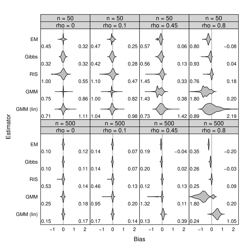
Figure 1: The distribution of the bias of the estimators of the autocorrelation parameter $\rho$ obtained from Monte Carlo simulations on 1,000 samples. Numbers represent minimum and maximum values of the bias.

The primary focus of this paper is on the estimation of the level of spatial autocorrelation in a binary spatial autoregressive model specification. Since we have the study of the diffusion of policies and regimes in mind, the level of diffusion is typically of key interest. The autocorrelation in the residuals is thus not treated as a mere nuisance, but as a structural factor of substantive interest. Figure 1 provides the distribution of the bias ofthe estimators of the spatial autocorrelation parameter $\rho$ in the BSAR model described in equation (3). Table 1 provides the mean and standard deviation of the bias of the above-mentioned estimators..

	$\rho=0$		$\rho=0.1$		$\rho=0.45$		$\rho=0.8$
	50	500	50	500	50	500	50	500
EM	-0.002	-0.002	-0.038	-0.016	-0.148	-0.104	-0.311	-0.272
	(0.108)	(0.034)	(0.108)	(0.030)	(0.107)	(0.022)	(0.098)	(0.023)
Gibbs	-0.017	-0.003	-0.050	-0.023	-0.114	-0.058	-0.140	-0.104
	(0.108)	(0.032)	(0.109)	(0.030)	(0.120)	(0.028)	(0.117)	(0.030)
RIS	-0.051	-0.002	-0.044	-0.003	-0.027	0.003	-0.015	-0.005
	(0.235)	(0.056)	(0.219)	(0.053)	(0.158)	(0.034)	(0.093)	(0.039)
GMM	0.019	-0.001	-0.049	-0.001	-0.243	-0.097	-0.547	-0.775
	(0.165)	(0.055)	(0.173)	(0.060)	(0.228)	(0.245)	(0.336)	(0.458)
GMM (lin)	0.011	-0.001	-0.037	-0.001	-0.075	0.080	0.028	0.468
	(0.149)	(0.043)	(0.166)	(0.044)	(0.232)	(0.072)	(0.528)	(0.205)

Table 1: The mean bias and the standard deviation (between parentheses) of the estimators of the autocorrelation parameter $\rho$ obtained from Monte Carlo simulations on 1,000 samples.

It is clear from Figure 1 that the performance of the estimators varies depending on the level of autocorrelation in the data, with particularly large differences between estimators under high levels of autocorrelation. As can be seen in Table 1, in the absence of spatial autocorrelation ($\rho=0$), the Gibbs and the EM estimators are the best estimators of $\rho$ in terms of both the distortion and the dispersion. The linearized GMM estimator also does particularly well, which is unsurprising, since $\rho=0$ is the value used as the starting point for the linearization. When looking at the distribution as a whole, however, it is clear that while this estimator performs generally well, there are clear outliers among the estimates. The RIS estimator shows the worst performance and it tends to underestimate $\rho$ for both small ($n=50$) and large ($n=500$) samples, with in particular some negative outliers. The Pinkse and Slade (1998) estimator, on the other hand, tends to overestimate $\rho$ in this scenario.

When the level of spatial autocorrelation is positive but still limited ($\rho=0.1$), the EM and Gibbs estimators still show good performance, even if the differences with the other estimators are less considerable in comparison with the scenario without spatial autocorrelation. Both the EM and the Gibbs estimators tend to underestimate the spatial autocorrelation parameter. As can be expected, the linearized GMM estimator is still performing well this close to the linearization point of $\rho=0$. The main disadvantage of this estimator is that it is not possible to put a reasonable constraint on $\hat{\rho}$, such that occasional estimates are obtained outside the $[-1,1]$ interval, visible in Figure 1. The RIS estimator is also prone to the occasional outlier in its estimate of the level of autocorrelation. It is striking that all estimators, with the exception of GMM with $n=50$, tend to underestimate $\rho$, often by over 50% of the true parameter value, when the sample size is low.

The next scenario contains significant levels of autocorrelation, with $\rho=0.45$. Under this level of autocorrelation, the RIS estimator starts to perform relatively well compared to the other estimators. While the absolute mean bias is the lowest, the variation is still relatively high, however, and the plot clearly shows the presence of some outliers. For the EM and the Gibbs estimators, the bias is significantly larger than for $\rho=0.1$ and for the linearized GMM, a clear increase in the dispersion is visible in Figure 1, although this is compensated by a reduction in extreme outliers. The distribution of the bias of the GMM estimator now shows a clear tendency to underestimate the amount of autocorrelation, with a tight distribution under $n=500$, but with some outliers.

For high spatial autocorrelation ($\rho=0.8$), the RIS estimator shows the best performance. The linearized GMM now clearly suffers from the large distance from the starting point of the linearization – the extrapolation from $\rho=0$ to $\rho=0.8$ leads to significant overestimation of the level of autocorrelation. The plot also shows that the estimator clearly suffers from the lack of a constraint on $\rho$. The GMM estimator shows rather significant underestimation of $\rho$, as well as a high level of variance. Furthermore, under this scenario, the simulations suggest asymptotically biased in mean results for the GMM and the linearized GMM estimators, with the mean bias increasing for the larger sample size. Following the trend already visible when moderately increasing $\rho$, the EM estimator clearly shows greater mean bias under this scenario, while for Gibbs, the results are similar to $\rho=0.45$.

	$\rho=0$		$\rho=0.1$		$\rho=0.45$		$\rho=0.8$
	50	500	50	500	50	500	50	500
EM	-59.23	-0.12	-43.12	-0.02	-5.52	1.03	1.42	1.69
	(507.24)	(0.34)	(356.69)	(0.33)	(56.98)	(0.11)	(3.64)	(0.03)
Gibbs	-0.95	-0.07	-0.86	-0.05	-0.63	0.09	0.30	0.79
	(1.12)	(0.28)	(1.09)	(0.29)	(1.02)	(0.24)	(0.70)	(0.19)
RIS	-8.05	0.01	-5.86	0.02	-6.86	0.13	-4.13	1.12
	(19.89)	(0.38)	(13.06)	(0.40)	(18.59)	(0.43)	(12.62)	(0.49)
GMM	-5035.95	-695.99	-4194.69	-576.70	-4777.75	-17864.07	-2818.31	-80663.45
	(28279.94)	(6344.00)	(23060.63)	(5841.52)	(15011.28)	(250693.49)	(11646.26)	(336721.33)
GMM (lin)	-64.15	-0.04	-41.08	0.07	-8.32	1.13	1.25	1.70
	(424.80)	(1.65)	(175.62)	(1.93)	(95.09)	(0.49)	(6.82)	(0.05)

Table 2: The mean bias and the standard deviation (between parentheses) of the estimators of the parameter $\beta_{1}$ obtained from Monte Carlo simulations on 1,000 samples.

Even with primary focus on the level of autocorrelation, the estimates of the effects of other independent variables can of course not be ignored. Table 2 provides the mean and the standard deviation of the estimates of $\beta_{1}$, the parameter for independent variable $X$. The differences in estimate accuracy between the estimators vary more dramatically than for $\rho$, with the Gibbs estimator clearly outperforming all other estimators under all conditions and the estimator proposed by Pinkse and Slade (1998) clearly providing the worst results for both the bias and the dispersion.

Under absence of spatial autocorrelation ($\rho=0$) and for $n=50$, the Gibbs estimator generates the least average bias on $\hat{\beta_{1}}$, with RIS, linearized GMM, and EM also performing well as long as the sample size is sufficiently large. Under $n=50$, the Gibbs estimator underestimates $\beta_{1}$ by about 50% on average of the value of $\beta_{1}$ and the other estimators well beyond that. The difference between the smaller and the larger sample sizes is more pronounced than for the estimates of $\rho$. The GMM estimator is the only estimator that is still significantly biased when the sample size is reasonably large. All estimators tend to underestimate $\beta_{1}$.

Under limited autocorrelation ($\rho=0.1$), the order of accuracy of the estimators remains more or less the same, with still only Gibbs performing the best under the small sample size and performing the well under the large sample size. The RIS performs similar to EM, Gibbs and GMMlin for large sample size. The GMM estimator shows the worst performance. Increasing the autocorrelation to $\rho=0.45$, the results for the Gibbs, the RIS and the GMM estimators are very similar to $\rho=0.1$, but the EM and the linearized GMM estimators show lower mean biases under small sample size.

For the estimation of $\rho$, we saw significant difference between the moderate and the high levels of autocorrelation – to what extent is this the case for the slope coefficients? Similar to the estimates of $\rho$, the GMM estimator of Pinkse and Slade (1998) starts to show very significant distortion and dispersion when the autocorrelation is high and, furthermore, shows a significant increase in the mean bias when the sample size increases. The linearized version of this estimator also reflects this increasing mean bias with sample size for high autocorrelation, but nevertheless performs remarkably well, with an average bias of approximately 50 to 75% of $\beta_{1}$, underestimating the magnitude of the negative effect of $X$. The Gibbs estimator outperforms all other estimators both with small and large sample sizes, followed by the RIS, the EM and the linearized GMM estimators as long as sample size is large. It should be noted that for all estimators, the bias is relatively large, which is an overestimate of the magnitude by slightly over 10%.

	$\rho=0$		$\rho=0.1$		$\rho=0.45$		$\rho=0.8$
	50	500	50	500	50	500	50	500
EM	121.85	0.24	85.58	0.05	12.52	-2.06	-3.02	-3.39
	(1120.25)	(0.70)	(689.86)	(0.69)	(127.40)	(0.23)	(11.82)	(0.11)
Gibbs	1.92	0.13	1.72	0.09	1.25	-0.19	-0.62	-1.58
	(2.44)	(0.59)	(2.34)	(0.60)	(2.21)	(0.50)	(1.68)	(0.39)
RIS	15.59	-0.01	11.62	-0.04	13.41	-0.26	8.14	-2.29
	(38.42)	(0.80)	(26.16)	(0.82)	(36.16)	(0.87)	(25.25)	(1.03)
GMM	10553.11	1497.72	8927.67	1215.51	9761.46	21968.93	5390.80	48233.04
	(57014.77)	(13763.26)	(46734.98)	(12202.29)	(30576.23)	(293214.42)	(26072.56)	(214363.69)
GMM (lin)	122.91	0.09	81.80	-0.13	17.71	-2.26	-2.72	-3.41
	(725.66)	(3.30)	(340.99)	(3.88)	(202.43)	(1.01)	(22.23)	(0.22)

Table 3: The mean bias and the standard deviation (between parentheses) of the estimators of the parameter $\beta_{0}$ obtained from Monte Carlo simulations on 1,000 samples.

Usually of least concern to applied researchers, but relevant for accurate prediction, is the estimate of the intercept of the model, in this case $\beta_{0}$. Table 3 provides the simulation results for this parameter of the model. Not unsurprisingly, the results are closely in line with those for $\beta_{1}$. Indeed, the mean of the bias of $\beta_{0}$ is roughly the bias in Table 2 multiplied by a factor $-2$. Relative to the size of $\beta$, the bias is thus the same on average. Similarly, the standard deviation of the bias is multiplied by a factor $2$, with the exception of the GMM estimator under higher levels of autocorrelation, where the dispersion under larger sample size is similar to that for $\beta_{1}$. The same relative results for the different estimators are therefore obtained.

5 Conclusion

In this paper we provide a comprehensive overview of estimators for spatial autoregressive models with binary dependent variables. These models are of particular interest to various applications in economics, political science, and related disciplines, where the outcome might be a policy, a decision, a transition, or otherwise binary outcome. Applications can also be imagined in the field of bioinformatics or neuroscience, although sample sizes tend to be magnitudes larger than those studied here. Many of these outcomes are interdependent through either spatial contiguity or any other form of proximity, including social networks or economic linkages, and ignoring the inherent spatial structure of the data generates inconsistent and inefficient estimates (McMillen, 1992). Furthermore, in many applications the researcher is explicitly concerned with estimating the level of interdependence – it is indeed this concern that is of primary interest in our discussion and simulation study.

This paper compares five estimators introduced to date for this specific type of model. An extensive simulation study compares the performance of these five estimators under conditions of relatively small sample sizes and varying levels of spatial autocorrelation. When taking both the estimation of the extend of spatial autocorrelation and the coefficients on the other explanatory variables into account, the Gibbs estimator (LeSage, 2000) clearly outperforms the other estimators. When the sample size increases, the difference between the different estimators becomes smaller. When focusing specifically on the spatial autoregressive component alone, the Gibbs estimator (LeSage, 2000) performs best for low spatial autocorrelation, while the Recursive Importance Sampler (Beron and Vijverberg, 2004) performs best for high spatial autocorrelation. The linearized GMM estimator (Klier and McMillen, 2008) is an interesting option when the sample size is large and the autocorrelation relatively low, in particular due to its high computational speed.

Appendix: Derivative for the linearization of the GMM BSAR model

The gradient (16) of interest to the linearization proposed in Klier and McMillen (2008) is the derivative of the logistic link function to the spatial autoregressive parameter $\rho$:

$$G_{\rho i}=\frac{\partial P_{i}}{\partial\rho}=\frac{\partial}{\partial\rho}\left[1+exp\left(q_{i}\right)\right]^{-1}=\frac{\partial}{\partial\rho}\left[1+exp\left(\frac{-{\bm{\Psi}}^{-1}{\mathbf{x}}_{i}^{\prime}{\bm{\beta}}}{\sigma_{ei}}\right)\right]^{-1},$$

where ${\bm{\Psi}}=({\mathbf{I}}-\rho{\mathbf{W}})$ and ${\mathbf{q}}$ as in equation (7). We derive the following gradient

$$G_{\rho i}=P_{i}(1-P_{i})\left(h_{i}+\frac{q_{i}}{\sigma_{ei}}\frac{\partial\sigma_{ei}}{\partial\rho}\right),$$

where ${\bm{h}}$ is defined in equation (16) and

$$\frac{\partial\sigma_{ei}}{\partial\rho} =\frac{\partial}{\partial\rho}\left[({\bm{\Psi}}^{\prime}{\bm{\Psi}})^{-1}\right]^{\frac{1}{2}}$$

$$=-\frac{1}{2\sigma_{ei}}({\bm{\Psi}}^{\prime}{\bm{\Psi}})^{-1}({\bm{\Psi}}+{\bm{\Psi}}^{\prime}){\mathbf{W}}({\bm{\Psi}}^{\prime}{\bm{\Psi}})^{-1}.$$ (17)

If ${\bm{\Psi}}$ is symmetric, equation (17) simplifies to:

$$\frac{\partial\sigma_{ei}}{\partial\rho} =-\frac{1}{\sigma_{ei}}{\bm{\Psi}}^{-1}{\mathbf{W}}{\bm{\Psi}}^{-1}{\bm{\Psi}}^{-1},$$

which leads to equation (16).

References

- (1)
- Albert and Chib (1993) Albert, J.H. and S. Chib. 1993. “Bayesian analysis of binary and polychotomous response data.” Journal of the American Statistical Association .
- Amemiya (1985) Amemiya, Takeshi. 1985. Advanced econometrics. Cambridge: Harvard University Press.
- Anselin (1982) Anselin, Luc. 1982. “A note on small sample properties of estimators in a first-order spatial autoregressive model.” Environment and Planning 14(1):1023–1030.
- Anselin (1988) Anselin, Luc. 1988. Spatial econometrics: methods and models. Dordrecht: Kluwer Academic Publishers.
- Anselin (2002) Anselin, Luc. 2002. “Under the hood. Issues in the specification and interpretation of spatial regression models.” Agricultural Economics 27:247–267.
- Anselin, Florax and Rey (2004) Anselin, Luc, Raymond J.G.M. Florax and Sergio J. Rey. 2004. Econometrics for Spatial Models: Recent Advances. In Advances in Spatial econometrics, ed. Luc Anselin, Raymond J.G.M. Florax and Sergio J. Rey. Berlin: Springer pp. 1–28.
- Autant-Bernard (2006) Autant-Bernard, Corinne. 2006. “Where do firms choose to locate their R&D? A spatial conditional logit analysis on French data.” European Planning Studies 14(9):1187–1208.
- Baturo and Gray (2009) Baturo, Alexander and Julia Gray. 2009. “Flatliners: Ideology and rational learning in the adoption of the flat tax.” European Journal of Political Research 48:130–159.
- Bee and Espa (2008) Bee, Marco and Giuseppe Espa. 2008. “A Monte Carlo EM algorithm for the estimation of a logistic auto-logistic model with missing data.” Letters in Spatial and Resource Sciences 1:45–54.
- Beron, Murdoch and Vijverberg (2003) Beron, Kurt J., James C. Murdoch and Wim P.M. Vijverberg. 2003. “Why cooperate? Public goods, economic power, and the Montreal protocol.” Review of Economics and Statistics 85(2):286–297.