Extensions of the time-dependent density functional based tight-binding approach

Abstract

The time-dependent density functional based tight-binding (TD-DFTB) approach is generalized to account for fractional occupations. In addition, an on-site correction leads to marked qualitative and quantitative improvements over the original method. Especially, the known failure of TD-DFTB for the description of $\sigma\rightarrow\pi^{*}$ and $n\rightarrow\pi^{*}$ excitations is overcome. Benchmark calculations on a large set of organic molecules also indicate a better description of triplet states. The accuracy of the revised TD-DFTB method is found to be similar to first principles TD-DFT calculations at a highly reduced computational cost. As a side issue, we also discuss the generalization of the TD-DFTB method to spin-polarized systems. In contrast to an earlier study [Trani et al., JCTC 7 3304 (2011)], we obtain a formalism that is fully consistent with the use of local exchange-correlation functionals in the ground state DFTB method.

I INTRODUCTION

During the last years, Density Functional Theory (DFT) has been one of the most utilized tools for the description of ground-state properties of a wide variety of molecular systems that range from small molecules to large periodic materials. While it lacks the accuracy typical of correlated wavefunction-based methods, it goes beyond Hartree-Fock (HF) as electron correlation is incorporated in a self-consistent-field (SCF) fashion. Thus, DFT has turned out to be a good compromise between accuracy and computational cost; affordable to study hundreds-of-atoms systems on most of the current work stations with fairly good precision. The field of application of this method was subsequently extended to the study of excited states properties with the development of time dependent density functional theory (TD-DFT).Runge and Gross (1984) This method has become the de facto standard for the computation of optical properties for molecules with several tens of atoms. Also the limitations of TD-DFT are now well documented in the literature (see e.g. Casida and Huix-Rotllant (2012)), which allows researchers to judge a priori whether a certain class of exchange-correlation functionals is sufficient for the predictive simulation of the problem at hand.

Still, many applications in photochemistry and nanophysics are not easily tractable in the current methodological frame. As an example, quantum molecular dynamics in the excited state require the evaluation of energies and forces at a large number of points along the trajectory. Also, the investigation of extended nanostructures like nanowires and -tubes with intrinsic defects or surface modifications can not be reliably performed with small models. For these kind of problems an approximate TD-DFT method might be advantageous. Such a scheme is the time dependent density functional based tight binding method (TD-DFTB).Niehaus et al. (2001) In the TD-DFTB method additional approximations beyond the choice of a given exchange-correlation functional are performed to enhance the numerical efficiency. These are mostly the neglect and simplification of two-electron integrals occurring in the linear response formulation of TD-DFT. In contrast to HF-based semi-empirical methods (like INDO/S or CIS-PM3), TD-DFTB approximates a reference method that already covers electronic correlation and does not include free parameters that are adjusted to reproduce experimental data.

After the original linear response implementation,Niehaus et al. (2001) TD-DFTB was extended in a number of different directions. Analytical excited state gradients have been derived,Heringer et al. (2007) as well as a real time propagation of Kohn-Sham (KS) orbitals that enables the computation of optical spectra using order-N algorithms.Yam et al. (2003) Several groups worked on non-adiabatic molecular dynamics simulations in the Ehrenfest Niehaus et al. (2005) or surface hopping Mitric et al. (2009); Jakowski et al. (2012) approach. More recent developments include a TD-DFTB approach for open boundary conditions in the field of quantum transport,Wang et al. (2011) as well as an implementation for open shell systems.Trani et al. (2011) A detailed review that summarizes advantages and limits of the method is also available.Niehaus (2009)

One of these limits is the rather poor description of $\sigma\rightarrow\pi^{*}$ and $n\rightarrow\pi^{*}$ excitations in many chromophores. In TD-DFTB these transitions show vanishing oscillator strengths although higher levels of theory clearly predict a finite (albeit small) transition probability. Moreover, singlet-triplet gaps for these kind of excitations are exactly zero in TD-DFTB, which is again in disagreement with more accurate methods. Although $\pi\rightarrow\pi^{*}$ transitions usually dominate the absorption spectrum, such low-lying excitations may play a significant role in the luminescence properties that are of key importance in many technological applications.

In this paper, we present extensions of the TD-DFTB method in order to improve its description of the absorption spectra of molecules. In the first section, the spin-unrestricted DFTB formulation for the ground state is briefly reviewed. Afterwards, we generalize the TD-DFTB approach for the study of open-shell systems with fractional occupancy. In IV, a refinement to overcome important deficiencies within the method is formulated. In order to highlight the qualitative improvement due to these extensions, we report results for selected diatomic molecules in V. Additionally, a comparison between results obtained with the proposed formalism and the original TD-DFTB approach for a large set of benchmark molecules is presented. Our findings are further compared to TD-DFT, the best theoretical estimates from the literature and experimental observations.

II Spin-unrestricted DFTB for the ground state

This section contains a brief summary of the spin-unrestricted DFTB method in order to establish the required notation for the later parts. More details on the derivation and application of the method are given in the original article by Köhler and co-workers.Köhler et al. (2001)

DFTB is based on a expansion of the DFT-KS energy up to the second order in the charge density fluctuations, $\delta\rho=\delta\rho_{\uparrow}+\delta\rho_{\downarrow}$, around a reference density, $\rho_{0}=\left[\rho_{0\uparrow},\rho_{0\downarrow}\right]$. The latter is given by a superposition of pre-calculated densities for neutral spin-unpolarized atoms. The DFTB energy reads:

$$E = \sum_{\sigma}\sum_{i}n_{i\sigma}\langle\psi_{i\sigma}|\hat{H}^{0}|\psi_{i\sigma}\rangle$$ (1)

$$+\frac{1}{2}\sum_{\sigma\tau}\iint\delta\rho_{\sigma}(\mathbf{r})\,f^{\text{hxc}}_{\rho_{\sigma}\rho_{\tau}}[\rho_{0}](\mathbf{r},\mathbf{r^{\prime}})\,\delta\rho_{\tau}(\mathbf{r}^{\prime})\,d\mathbf{r}d\mathbf{r}^{\prime}+E_{\text{rep}},$$

where the $n_{i\sigma}$ denote occupation numbers, $E_{\text{rep}}$ is a sum of pair potentials independent of the electronic density,Frauenheim et al. (2002) and $f^{\text{hxc}}=f^{\text{h}}+f^{\text{xc}}$ with

$$f^{\text{h}}(\mathbf{r},\mathbf{r^{\prime}}) = \frac{1}{|\mathbf{r}-\mathbf{r}^{\prime}|}$$

$$f^{\text{xc}}_{\rho_{\sigma}\rho_{\tau}}[\rho](\mathbf{r},\mathbf{r^{\prime}}) = \frac{\delta^{2}E_{xc}[\rho]}{\delta\rho_{\sigma}(\mathbf{r})\delta\rho_{\tau}(\mathbf{r}^{\prime})},$$ (2)

denote the Coulomb and exchange-correlation kernel, respectively.

In the first (zeroth-order) term of 1, $\hat{H}^{0}$ is the KS Hamiltonian evaluated at $\rho_{0}$ and the sum runs over the spin variables $\sigma=\uparrow,\downarrow$ and the KS orbitals $\psi_{i\sigma}$. For the succeeding formulation, the Roman indices $s,t,u,v,$ denote KS orbitals, whereas Greek indices $\mu,\nu,\kappa,\lambda$ will denote atomic orbitals (AO). Let us also abbreviate a general two-point integral over a kernel $g(\mathbf{r},\mathbf{r^{\prime}})$ in the following form:

$$\left(f|g|h\right)=\iint f(\mathbf{r})g(\mathbf{r},\mathbf{r^{\prime}})h(\mathbf{r^{\prime}})\,d\mathbf{r}d\mathbf{r}^{\prime}.$$ (3)

For atomic orbital products $f(\mathbf{r})=\phi_{\mu}(\mathbf{r})\phi_{\nu}(\mathbf{r})$ and $h(\mathbf{r}^{\prime})=\phi_{\kappa}(\mathbf{r}^{\prime})\phi_{\lambda}(\mathbf{r}^{\prime})$ the shorthand $\left(\mu\nu|g|\kappa\lambda\right)$ will be also used. Expanding the KS orbitals (which we choose to be real) into a suitable set of such localized atom-centered AO, $\psi_{i\sigma}=\sum_{\mu}c_{\mu i}^{\sigma}\phi_{\mu}$, the second term in 1, labeled $E^{(2)}$ in the following, can be written as

$$E^{(2)}=\frac{1}{2}\sum_{\sigma\tau}\sum_{\mu\nu\kappa\lambda}\Delta P_{\mu\nu}^{\sigma}\left(\mu\nu|f^{\text{hxc}}_{\rho_{\sigma}\rho_{\tau}}[\rho_{0}]|\kappa\lambda\right)\Delta P_{\kappa\lambda}^{\tau},$$ (4)

where $\Delta P_{\mu\nu}^{\sigma}=P_{\mu\nu}^{\sigma}-P_{\mu\nu}^{0,\sigma}$ denotes the AO density matrix of the difference density $\delta\rho_{\sigma}(\mathbf{r})$, with

$$P_{\mu\nu}^{\sigma}=\sum_{st}c_{\mu s}^{\sigma}P_{st}^{\sigma}c_{\nu t}^{\sigma},~{}~{}~{}P_{\mu\nu}^{0,\sigma}=\sum_{st}c_{\mu s}^{\sigma}P_{st}^{0,\sigma}c_{\nu t}^{\sigma}.$$ (5)

Here $P_{st}^{\sigma}=\langle\Psi|\hat{a}_{t\sigma}^{\dagger}\hat{a}_{s\sigma}|\Psi\rangle$ are the MO density matrix elements, $\Psi$ being the ground state KS determinant. The term $P_{st}^{0,\sigma}$ designates the MO density matrix of the reference system.

To evaluate the appearing integrals, the Mulliken approximation is applied. This amounts to set $\phi_{\mu}\phi_{\nu}\approx\frac{1}{2}S_{\mu\nu}(|\phi_{\mu}|^{2}+|\phi_{\nu}|^{2})$, using the known AO overlap integrals $S_{\mu\nu}$. Thus, the general four-center integrals are written in terms of two-center integrals,

$$\left(\mu\nu|f^{\text{hxc}}_{\rho_{\sigma}\rho_{\tau}}[\rho_{0}]|\kappa\lambda\right)\approx\frac{1}{4}S_{\mu\nu}S_{\kappa\lambda}\sum_{\alpha\in\{\mu,\nu\}}\sum_{\beta\in\{\kappa,\lambda\}}\left(\alpha\alpha|f^{\text{hxc}}_{\rho_{\sigma}\rho_{\tau}}[\rho_{0}]|\beta\beta\right).$$ (6)

By substituting 6 into 4, the second order contribution to the energy reads,

$$E^{(2)}=\frac{1}{2}\sum_{\sigma\tau}\sum_{\mu\nu}\Delta\tilde{P}_{\mu\mu}^{\sigma}\left(\mu\mu|f^{\text{hxc}}_{\rho_{\sigma}\rho_{\tau}}[\rho_{0}]|\nu\nu\right)\Delta\tilde{P}_{\nu\nu}^{\tau},$$ (7)

where $\tilde{P}_{\mu\nu}^{\sigma}$ are the elements of the dual density matrix defined as

$$\tilde{\mathbf{P}}=\frac{1}{2}\left(\mathbf{P}\cdot\mathbf{S}+\mathbf{S}\cdot\mathbf{P}\right).$$ (8)

By using 5, the dual density matrix can be expressed with respect to the MO density matrix as

$$\tilde{P}_{\mu\nu}^{\sigma}=\sum_{st}P_{\mu\nu}^{st\sigma}P_{st}^{\sigma}.$$ (9)

The matrix $P_{\mu\nu}^{st\sigma}$ represents the Kohn-Sham transition density for an excitation from orbital s to t, and is defined as follows:

$$P_{\mu\nu}^{st\sigma}=\frac{1}{4}\left(c_{\mu s}^{\sigma}\tilde{c}_{\nu t}^{\sigma}+c_{\mu t}^{\sigma}\tilde{c}_{\nu s}^{\sigma}+c_{\nu s}^{\sigma}\tilde{c}_{\mu t}^{\sigma}+c_{\nu t}^{\sigma}\tilde{c}_{\mu s}^{\sigma}\right),~{}~{}\tilde{\mathbf{c}}_{s}=\mathbf{c}_{s}\cdot\mathbf{S}.$$ (10)

A further simplification to 7 is obtained by spherical averaging over AO products. This ensures that the final total energy expression is invariant with respect to arbitrary rotations of the molecular frame. To this end, the functions $F_{Al}$ are introduced

$$F_{Al}(|{\bf r}-\mathbf{R}_{A}|)=\frac{1}{2l+1}\sum_{m=-l}^{m=l}|\phi_{\mu}({\bf r}-\mathbf{R}_{A})|^{2},$$ (11)

where $l$ and $m$ denote the angular momentum and magnetic quantum number of AO $\phi_{\mu}$, centered on atom $A$. We then have for $\mu=\{Alm\}$, $\nu=\{Bl^{\prime}m^{\prime}\}$:

$$\left(\mu\mu|f^{\text{hxc}}_{\rho_{\sigma}\rho_{\tau}}[\rho_{0}]|\nu\nu\right)\approx\left(F_{Al}|f^{\text{hxc}}_{\rho_{\sigma}\rho_{\tau}}[\rho_{0}]|F_{Bl^{\prime}}\right)=\Gamma_{Al,Bl^{\prime}}^{\sigma\tau}$$ (12)

introducing the shorthand notation $\Gamma$.

The traditional DFTB energy expression is now obtained after transformation from the set $\{\rho_{\uparrow},\rho_{\downarrow}\}$ to the total density $\rho=\rho_{\uparrow}+\rho_{\downarrow}$ and magnetization $m=\rho_{\uparrow}-\rho_{\downarrow}$. By this change of variables, the exchange-correlation kernel can be split and one arrives at

$$\Gamma_{Al,Bl^{\prime}}^{\sigma\tau}=\gamma_{Al,Bl^{\prime}}+\delta_{\sigma}\delta_{\tau}\delta_{AB}W_{Al,l^{\prime}},$$ (13)

where $\delta_{\sigma}=2\delta_{\sigma\uparrow}-1$ and the parameters $\gamma_{Al,Bl^{\prime}}=\left(F_{Al}|f^{\text{hxc}}_{\rho\rho}[\rho_{0}]|F_{Bl^{\prime}}\right)$ and $W_{Al,l^{\prime}}=\left(F_{Al}|f^{\text{xc}}_{mm}[\rho_{0}]|F_{Al^{\prime}}\right)$. Please note that the constants $W_{Al,l^{\prime}}$ depend only on the exchange-correlation kernel, but not on the long-range Coulomb interaction. Moreover, as the reference density $\rho_{0}$ is built from neutral spin-unpolarized atomic densities, there are no integrals which involve mixed derivatives of the exchange-correlation energy with respect to both density and magnetization. The parameters $\gamma_{Al,Bl^{\prime}}$ and $W_{Al,l^{\prime}}$ are known in the DFTB method as the $\gamma$-functional and spin coupling constants, respectively.Frauenheim et al. (2002) The spin coupling constants are treated as strictly on-site parameters, whereas $\gamma$ is calculated for every atom pair using an interpolation formula, that depends on the distance between the atoms $A$ and $B$ and the atomic Hubbard-like parameters $\gamma_{Al,Al}$ and $\gamma_{Bl,Bl}$. Traditionally, the latter are not computed directly from the integral 12, but from total energy derivatives according to $\gamma_{Al,Al}=\delta^{2}E/\delta n^{2}$. In this expression, $E$ denotes the DFT total energy of atom $A$ and $n$ refers to the occupation of the shell with angular momentum $l$. The derivative is then evaluated numerically by full self-consistent field calculations at perturbed occupations. Due to orbital relaxation, parameters obtained in this way are roughly 10-20 % smaller than the ones from a direct integral evaluation. This point will become important later.

Finally, by substituting 9 in 7 while using 12, the second order energy term can be expressed as

$$E^{(2)}=\frac{1}{2}\sum_{\sigma\tau}\sum_{stuv}\sum_{ABll^{\prime}}\Delta P_{st}^{\sigma}q_{Al}^{st\sigma}\Gamma_{Al,Bl^{\prime}}^{\sigma\tau}q_{Bl^{\prime}}^{uv\tau}\Delta P_{uv}^{\tau},$$ (14)

where $q_{Al}^{st\sigma}=\sum_{\mu\in A,l}P_{\mu\mu}^{st\sigma}$ are the angular-momentum-resolved transition charges for atom $A$. For later reference, we next define a matrix $\bar{\mathbf{K}}$:

$$\bar{K}_{st\sigma,uv\tau}=\sum_{ABll^{\prime}}q_{Al}^{st\sigma}\Gamma_{Al,Bl^{\prime}}^{\sigma\tau}q_{Bl^{\prime}}^{uv\tau}.$$ (15)

Using this abbreviation, the DFTB total energy can then be written in the following simple form,

$$E = \sum_{\sigma}\sum_{st}H_{st\sigma}^{0}P_{st}^{\sigma}+\frac{1}{2}\sum_{\sigma\tau}\sum_{stuv}\Delta P_{st}^{\sigma}\bar{K}_{st\sigma,uv\tau}\Delta P_{uv}^{\tau}+E_{\text{rep}}.$$ (16)

By applying the variational principle to the energy functional, the DFTB KS equations are obtained

$$H_{st\sigma}-\epsilon_{s\sigma}\delta_{st}=0,~{}~{}\forall s,t,\sigma$$ (17)

where the KS Hamiltonian is expressed as

$$H_{st\sigma}=\frac{\partial E}{\partial P_{st}^{\sigma}}=H_{st\sigma}^{0}+\sum_{\tau}\sum_{uv}\bar{K}_{st\sigma,uv\tau}\Delta P_{uv}^{\tau}.$$ (18)

These equations are subsequently transformed into a set of algebraic equations by expanding the KS orbitals into the AO basis, and are solved self-consistently. For the converged ground state density we have $P_{st}^{\sigma}=n_{s\sigma}\delta_{st}$. Using also the identity $\sum_{st}c_{\mu s}^{\sigma}P_{st}^{0,\sigma}c_{\nu t}^{\sigma}=n^{0}_{\mu\sigma}\delta_{\mu\nu}~{}(\forall\mu,\nu,\sigma)$, $n^{0}_{\mu\sigma}$ being the occupation numbers for the reference atoms, it is straightforward to recover the expression for the spin-unrestricted DFTB Hamiltonian given in Köhler et al. (2001); Frauenheim et al. (2002).

III Spin-unrestricted TD-DFTB

Once the KS orbitals $\psi_{i\sigma}$ and energies $\epsilon_{i\sigma}$ are obtained, a linear density-response treatment directly applies as a natural extension to DFTB. Following Casida,Casida (1995) the excitation energies $\omega_{I}$ and eigenvectors $F_{I}$ can be calculated by solving the eigenvalue problem

$$\boldsymbol{\Omega}\mathbf{F}_{I}=\omega_{I}^{2}\mathbf{F}_{I},$$ (19)

where the response matrix $\boldsymbol{\Omega}$ is defined as

$$\boldsymbol{\Omega}=\mathbf{S}^{-1/2}\left(\mathbf{A}+\mathbf{B}\right)\mathbf{S}^{-1/2}$$ (20)

$$\mathbf{S}=-\mathbf{C}\left(\mathbf{A}-\mathbf{B}\right)^{-1}\mathbf{C}.$$ (21)

The matrices $\mathbf{A}$, $\mathbf{B}$ and $\mathbf{C}$ are defined according to

$$A_{ia\sigma,jb\tau} = \frac{\delta_{ij}\delta_{ab}\delta_{\sigma\tau}\omega_{jb\tau}}{n_{j\tau}-n_{b\tau}}+K_{ia\sigma,jb\tau}$$

$$B_{ia\sigma,jb\tau} = K_{ia\sigma,bj\tau}$$

$$C_{ia\sigma,jb\tau} = \frac{\delta_{ij}\delta_{ab}\delta_{\sigma\tau}}{n_{j\tau}-n_{b\tau}},$$ (22)

where $\omega_{jb\tau}=\epsilon_{b\tau}-\epsilon_{j\tau}$ and the indexes $i,j,a,b$ stand for KS orbitals such that $n_{i\sigma}>n_{a\sigma}$ and $n_{j\tau}>n_{b\tau}$. We explicitly allow for fractional occupations at this point in order to be able to simulate also metallic or near-metallic systems at elevated electronic temperature.

The coupling matrix elements $K_{ia\sigma,jb\tau}$ are generally defined as the derivative of the KS Hamiltonian with respect to the density matrix elements. For the special case of DFTB (see 18), this leads to the matrix $\bar{\mathbf{K}}$ defined in 15

$$K_{ia\sigma,jb\tau}:=\frac{\partial H_{ia\sigma}}{\partial P_{jb}^{\tau}}=\bar{K}_{ia\sigma,jb\tau}.$$ (23)

This quantity depends only on the $\gamma$ and $W$ parameters, as well as on the Mulliken transitions charges obtained from the previous ground state DFTB calculation.

An important feature of the coupling matrix for local or semi-local exchange-correlation functionals is its invariance with respect to the permutation of any connected (real orbital) indices (e.g. $K_{ia\sigma,jb\tau}=K_{ia\sigma,bj\tau}=K_{ai\sigma,jb\tau}$). This symmetry does not hold for functionals involving Hartree-Fock exchange.Casida (1995) In contrast to an earlier derivation,Trani et al. (2011) we find that the DFTB coupling matrix is in fact symmetric. This can be traced back to the transition density matrix, 10, that evidently has this property. Since the ground state DFTB method is derived as an approximation to local or semi-local DFT only, this is an expected and necessary property and implies that the orbital rotation Hessian $\mathbf{A}-\mathbf{B}$ becomes strictly diagonal. Thus, the expression for the response matrix elements is conveniently simplified to read

$$\Omega_{ia\sigma,jb\tau}=\delta_{ij}\delta_{ab}\delta_{\sigma\tau}\omega_{jb\tau}^{2}+2\sqrt{\left(n_{i\sigma}-n_{a\sigma}\right)\omega_{ia\sigma}}K_{ia\sigma,jb\tau}\sqrt{\left(n_{j\tau}-n_{b\tau}\right)\omega_{jb\tau}}.$$ (24)

It is worth formulating the method for closed shell systems as a particular case, in order to make contact with the original derivation of TD-DFTB . In this special case the Mulliken transition charges have the property $q_{Al}^{ia\uparrow}=q_{Al}^{ia\downarrow}=q_{Al}^{ia}$. If, in addition, the dependence of the $\gamma$-functional and $W$ constants on the angular momentum is neglected, the coupling matrix simplifies to

$$K_{ia\sigma,jb\tau}=\sum_{AB}q_{A}^{ia}\left(\gamma_{AB}+\delta_{\sigma}\delta_{\tau}\delta_{AB}W_{A}\right)q_{B}^{jb},$$ (25)

with $q_{A}^{ia}=\sum_{l}q_{Al}^{ia}$, in full agreement with the expression derived previously for spin-unpolarized densities.Niehaus et al. (2001)

Once the eigenvalue problem is solved within TD-DFTB, the oscillator strength related to excitation $I$ can be calculated as

$$f^{I}=\frac{2}{3}\sum_{k=1}^{3}\left|\sum_{ia\sigma}\langle\psi_{i\sigma}|\hat{r}_{k}|\psi_{a\sigma}\rangle\sqrt{\left(n_{i\sigma}-n_{a\sigma}\right)\omega_{ia\sigma}}F_{ia\sigma}^{I}\right|^{2},$$ (26)

where $\hat{r}_{k}$ denotes the $k$-th component of the position operator. The transition-dipole matrix elements are also subjected to a Mulliken approximation ($\mathbf{R}_{A}$ is the position of atom $A$):

$$\langle\psi_{i\sigma}|\hat{\mathbf{r}}|\psi_{a\sigma}\rangle\approx\sum_{A}\mathbf{R}_{A}q_{A}^{ia\sigma}.$$ (27)

IV Beyond the Mulliken approximation

While in general the Mulliken approximation accounts, at least approximately, for the differential overlap of atomic orbitals, there is an important exception. If orbitals $\phi_{\mu}$ and $\phi_{\nu}$ with $\mu\neq\nu$ reside on the same atom, their product vanishes since the overlap matrix reduces to the identity. As a consequence, the transition charges are underestimated or often vanish identically for excitations that feature localized MO, e.g. $n\to\pi^{*}$ transitions. This in turn means that the coupling matrix vanishes and hence no correction of the ground state KS energy differences occurs in the linear response treatment. More importantly, the singlet-triplet gap is zero for such excitations.

A next level of approximation demands therefore the evaluation of all one-center integrals of the exchange type, i.e., $\left(\mu\nu|f^{\text{hxc}}_{\rho_{\sigma}\rho_{\tau}}[\rho_{0}]|\mu\nu\right)$ with $\mu\neq\nu$. This is how Pople et al. proceeded in the development of the intermediate neglect of differential overlap model (INDO) Pople et al. (1967) to overcome the deficiencies encountered within the complete neglect of differential overlap method (CNDO).Pople et al. (1965) Under the INDO model, the one-center, two-electron integrals are fitted to atomic spectroscopic data. In this work, the corresponding one-center integrals are calculated by numerical integration.

After inclusion of every onsite exchange-like integral within the DFTB formalism (see A), the second-order energy takes the new form:

$$E^{(2)} = \frac{1}{2}\sum_{\sigma\tau}\sum_{A}\sum_{\mu\nu\in A}\Delta\tilde{P}_{\mu\mu}^{\sigma}\left(\mu\mu|f^{\text{hxc}}_{\rho_{\sigma}\rho_{\tau}}[\rho_{0}]|\nu\nu\right)\Delta\tilde{P}_{\nu\nu}^{\tau}$$ (28)

$$+ \sum_{\sigma\tau}\sum_{A}\sum_{\mu\nu\in A}^{\mu\neq\nu}\Delta\tilde{P}_{\mu\nu}^{\sigma}\left(\mu\nu|f^{\text{hxc}}_{\rho_{\sigma}\rho_{\tau}}[\rho_{0}]|\mu\nu\right)\Delta\tilde{P}_{\mu\nu}^{\tau}$$

$$+ \frac{1}{2}\sum_{\sigma\tau}\sum_{AB}^{A\neq B}\sum_{\mu\in A}\sum_{\nu\in B}\Delta\tilde{P}_{\mu\mu}^{\sigma}\left(\mu\mu|f^{\text{hxc}}_{\rho_{\sigma}\rho_{\tau}}[\rho_{0}]|\nu\nu\right)\Delta\tilde{P}_{\nu\nu}^{\tau},$$

where the onsite integrals appear in the second term and the previous energy expression (7) has been split into on-site (first term) and off-site (third term) contributions.

By substituting 9 in 28 while using 12 for the off-site component, $E^{(2)}$ can be finally written as

$$E^{(2)}=\frac{1}{2}\sum_{\sigma\tau}\sum_{stuv}\Delta P_{st}^{\sigma}K_{st\sigma,uv\tau}\Delta P_{uv}^{\tau},$$ (29)

with the refined coupling matrix $\mathbf{K}$ being expressed as

$$K_{st\sigma,uv\tau} = \sum_{A}\sum_{\mu\nu\in A}P_{\mu\mu}^{st\sigma}\left(\mu\mu|f^{\text{hxc}}_{\rho_{\sigma}\rho_{\tau}}[\rho_{0}]|\nu\nu\right)P_{\nu\nu}^{uv\tau}$$ (30)

$$+ 2\sum_{A}\sum_{\mu\nu\in A}^{\mu\neq\nu}P_{\mu\nu}^{st\sigma}\left(\mu\nu|f^{\text{hxc}}_{\rho_{\sigma}\rho_{\tau}}[\rho_{0}]|\mu\nu\right)P_{\mu\nu}^{uv\tau}$$

$$+ \sum_{ABll^{\prime}}^{A\neq B}q_{Al}^{st\sigma}\Gamma_{Al,Bl^{\prime}}^{\sigma\tau}q_{Bl^{\prime}}^{uv\tau}.$$

With inclusion of the exchange integrals, the spherical averaging over AO products described in 12 will in general not lead to an expression which is invariant under a rotation of the atomic axes. This has been discussed by Figeys et. al,Figeys et al. (1977) who analyzed the rotational invariance (RI) of the INDO model. Taking p-type orbitals as an example, the following identity must hold to preserve RI:

$$(pp|f^{\text{hxc}}_{\rho_{\sigma}\rho_{\tau}}[\rho_{0}]|pp)-(pp|f^{\text{hxc}}_{\rho_{\sigma}\rho_{\tau}}[\rho_{0}]|p^{\prime}p^{\prime})=2(pp^{\prime}|f^{\text{hxc}}_{\rho_{\sigma}\rho_{\tau}}[\rho_{0}]|pp^{\prime}),~{}\forall p,p^{\prime}\,.$$ (31)

In the original DFTB formulation this requirement is fulfilled, as both integrals on the left-hand side of 31 are approximated to have the same value, $\Gamma_{Ap,Ap}^{\sigma\tau}$, while the integral on the right-hand side is neglected. To retain RI within the present scheme, one could evaluate all on-site integrals exactly so that 31 holds automatically. As detailed in II, the corresponding averaged $\Gamma$-parameters would then differ from the ones usually employed in ground state DFTB simulations, which are obtained from total energy derivatives. Instead, we use 31 to calculate all required parameters, taking the exact exchange integrals and the traditional $\Gamma$-parameters as input. In this way the modifications of the original method are kept as small as possible, while RI is still exactly preserved.

The eqs 29 and 30 represent a correction to the conventional DFTB energy expression, whose implication for various ground state properties certainly warrants a deeper investigation. Since we are mainly interested in an improvement of the TD-DFTB scheme at this point, we keep with the traditional DFTB scheme for the ground state and employ the modified coupling matrix only in the response part of the calculation, i.e. in 22.

In a similar manner as the refinement of the coupling matrix was achieved, the approximation for the dipole matrix elements eq 27, and hence the oscillator strength, can be improved by including all non-vanishing one-center dipole integrals (see B),

$$\langle\psi_{i\sigma}|\mathbf{\hat{r}}|\psi_{a\sigma}\rangle=\sum_{A}\mathbf{R}_{A}q_{A}^{ia\sigma}+\sum_{A}\sum_{\mu\nu\in A}^{\mu\neq\nu}P_{\mu\nu}^{ia\sigma}\langle\mu|\mathbf{\hat{r}}|\nu\rangle.$$ (32)

According to the dipole selection rules only $s$-$p$ and $p$-$d$ dipole integrals are non-zero. Among the $s$-$p$ integrals, only those of the type $D_{sp}=\langle s|r_{k}|p_{k}\rangle$ do not vanish, all of them being equal. With regards to the $p$-$d$ integrals, eleven of them are non-vanishing:

$$D_{pd} = \langle p_{y}|x|d_{xy}\rangle=\langle p_{x}|y|d_{xy}\rangle=\langle p_{y}|z|d_{yz}\rangle=\langle p_{z}|y|d_{yz}\rangle=\langle p_{z}|x|d_{xz}\rangle=\langle p_{x}|z|d_{xz}\rangle$$

$$D_{pd} = \langle p_{x}|x|d_{x^{2}-y^{2}}\rangle=-\langle p_{y}|y|d_{x^{2}-y^{2}}\rangle$$

$$D_{pd}^{\prime} = \langle p_{y}|y|d_{z^{2}}\rangle=\langle p_{x}|x|d_{z^{2}}\rangle$$

$$D_{pd}^{\prime\prime} = \langle p_{z}|z|d_{z^{2}}\rangle.$$ (33)

We would like to stress that the required additional atomic integrals in our correction to the coupling matrix and oscillator strength are neither freely adjustable parameters nor fitted to experiment. Instead, they are calculated numerically with a special-purpose DFT code that was recently developed in our group.

Like in earlier studies with the DFTB method, the Perdew-Burke-Ernzerhof (PBE) Perdew et al. (1996) functional was used in the calculation of Hamiltonian and overlap matrices, as well as the computation of reference densities and basis functions. This also holds for the new parameters, which are calculated once for every atom type, stored in a file, and read when needed during the calculation.

The presented extensions of the TD-DFTB method have been implemented in a development version of the DFTB+ code.Aradi et al. (2007)

V RESULTS

V.1 Diatomic molecules

To show the performance of our corrections to the coupling and dipole matrices (hereafter referred to as the onsite correction), we calculated the low-lying vertical excitation energies and their corresponding oscillator strengths of three diatomic molecules for which the improvements over traditional TD-DFTB are especially noticeable. It is important to point out that only valence excited states can be treated within TD-DFTB due to the employed minimal basis set. 1 shows the excitation energies of NO, N₂ and O₂ calculated within both the corrected and the original formulation of TD-DFTB. For NO and O₂, spin-unrestricted TD-DFTB calculations have been performed, where doublet and triplet ground states have been considered, respectively. In order to identify the excited state multiplicity of the open-shell systems, the expectation value of the square of the total spin operator, $\langle S^{2}\rangle$, is evaluated. We apply the expression derived in Ref. Maurice and Head-Gordon (1995) for unrestricted configuration interaction singles (UCIS) wave functions for this purpose. In 1, a multiplicity is only assigned to those excited states with low spin contamination. This covers the most important excitations in the absorption spectrum.

As a reference, we computed vertical excitation energies to valence states of these compounds by using TD-DFT as implemented in the TURBOMOLE package TUR . The PBE exchange-correlation functional as well as triple-zeta plus polarization (TZP) basis set has been used. All ground state geometries were previously optimized at the corresponding level of theory. Some experimental findings taken from the literature are also included for comparison Oddershede et al. (1985); Krupenie (1972). The oscillator strength for each excitation is indicated to the right of the corresponding excitation energy and in the first column of the table the symmetry and type of the transition is specified.

Molecule/Trans.	TD-DFT				TD-DFTB					Exp.
	$\omega_{I}$	$f_{I}$	$\omega_{\text{KS}}$		$\omega_{I}^{\text{new}}$	$f_{I}^{\text{new}}$	$\omega_{I}^{\text{old}}$	$f_{I}^{\text{old}}$	$\omega_{\text{KS}}$
NO
$~{}~{}~{}\Sigma^{+}$ ($\pi\rightarrow\pi^{*}$)	6.46	$<$0.01	8.36		7.22	$<$0.01	7.49	$<$0.01	8.53
$~{}~{}~{}\Pi^{~{}}$ ($\sigma\rightarrow\pi^{*}$)	6.49	$<$0.01	7.23		7.29	$<$0.01	7.77	0.00	7.80/7.77
$~{}~{}~{}\Delta_{~{}}$ ($\pi\rightarrow\pi^{*}$)	7.26	0.00	8.36		7.74	0.00	8.53	0.00	8.64/8.53
$~{}~{}~{}\Sigma^{-}$ ($\pi\rightarrow\pi^{*}$)	8.36	0.00	8.36		8.53	0.00	8.53	0.00	8.53
$~{}^{2}\Pi_{~{}}$ ($\sigma\rightarrow\pi^{*}$)	8.61	0.02	7.84		8.33	0.01	7.80	0.00	7.77/7.80
$~{}~{}~{}\Sigma^{-}$ ($\pi\rightarrow\pi^{*}$)	8.74	0.00	8.74		8.64	0.00	8.64	0.00	8.64
$~{}^{2}\Delta_{~{}}$ ($\pi\rightarrow\pi^{*}$)	9.11	0.00	8.74		9.09	0.00	8.64	0.00	8.64
$~{}~{}~{}\Pi_{~{}}$ ($\sigma^{*}\rightarrow\pi^{*}$)	11.64	$<$0.01	12.45		12.68	$<$0.01	13.19	0.00	13.19
$~{}^{2}\Sigma^{+}$ ($\pi\rightarrow\pi^{*}$)	14.00	0.35	8.47		11.90	0.63	11.65	0.50	8.64
$~{}^{2}\Pi_{~{}}$ ($\sigma^{*}\rightarrow\pi^{*}$)	14.82	0.38	12.87		14.64	0.24	13.23	0.00	13.23
N2
$~{}^{3}\Pi_{g}$ ($\sigma_{g}\rightarrow\pi_{g}$)	7.30		8.20		7.48		8.12		8.12	8.04
$~{}^{3}\Sigma_{u}^{+}$ ($\pi_{u}\rightarrow\pi_{g}$)	7.42		9.60		6.91		7.36		9.01	7.75
$~{}^{3}\Delta_{u}$ ($\pi_{u}\rightarrow\pi_{g}$)	8.24		9.60		7.76		9.01		9.01	8.88
$~{}^{3}\Sigma_{u}^{-}$ ($\pi_{u}\rightarrow\pi_{g}$)	9.60		9.60		9.01		9.01		9.01	9.67
$~{}^{3}\Pi_{u}$ ($\sigma_{u}\rightarrow\pi_{g}$)	10.37		11.49		11.30		12.06		12.06	11.19
$~{}^{1}\Pi_{g}$ ($\sigma_{g}\rightarrow\pi_{g}$)	9.05	0.00	8.20		8.71	0.00	8.12	0.00	8.12	9.31
$~{}^{1}\Sigma_{u}^{-}$ ($\pi_{u}\rightarrow\pi_{g}$)	9.60	0.00	9.60		9.01	0.00	9.01	0.00	9.01	9.92
$~{}^{1}\Delta_{u}$ ($\pi_{u}\rightarrow\pi_{g}$)	10.03	0.00	9.60		9.66	0.00	9.01	0.00	9.01	10.27
$~{}^{1}\Pi_{u}$ ($\sigma_{u}\rightarrow\pi_{g}$)	13.53	0.42	11.49		13.82	0.33	12.06	0.00	12.06	12.78
$~{}^{1}\Sigma_{u}^{+}$ ($\pi_{u}\rightarrow\pi_{g}$)	14.84	0.77	9.60		13.02	0.98	12.75	0.80	9.01	12.96
O2
$~{}^{3}\Delta_{u}$ ($\pi_{u}\rightarrow\pi_{g}$)	6.39	0.00	6.90		6.21	0.00	6.35	0.00	6.35	6.0-6.2
$~{}^{3}\Sigma_{u}^{-}$ ($\pi_{u}\rightarrow\pi_{g}$)	6.90	0.00	6.90		6.35	0.00	6.35	0.00	6.35	6.3-6.5
$~{}^{3}\Pi_{g}$ ($\sigma_{g}\rightarrow\pi_{g}$)	7.84	0.00	7.91		6.80	0.00	6.79	0.00	6.79
$~{}^{3}\Sigma_{u}^{+}$ ($\pi_{u}\rightarrow\pi_{g}$)	9.00	0.18	6.90		8.36	0.32	8.21	0.24	6.35	$\sim$8.6
$~{}^{3}\Pi_{u}$ ($\sigma_{u}\rightarrow\pi_{g}$)	14.85	0.18	14.16		15.35	0.18	14.52	0.00	14.52

Table 1: Comparison of vertical excitation energies $\omega_{I}$ and oscillator strengths $f_{I}$ for TD-DFT with TZP basis set, the traditional TD-DFTB method (old) and TD-DFTB with onsite correction (new). The PBE functional is used throughout. $\omega_{\text{KS}}$ denotes the KS orbital energy difference corresponding to the most dominant single particle transition in the many body wavefunction, as discussed by Casida in Ref. Casida (1995). Experimental data for N₂ and O₂ were taken from Ref. Oddershede et al. (1985) and inferred from the potential energy curves in Ref. Krupenie (1972), respectively. Oscillator strengths are only provided for excitations that are not trivially spin-forbidden. All energies are expressed in eV.

These molecules have as a common feature that they all possess low-lying $\sigma\rightarrow\pi^{*}$ excitations playing an important role in their absorption spectra. As stated above, a wrong description of these transitions is a known issue in current TD-DFTB. Below, we identify yet another failure in the description of some $\pi\rightarrow\pi^{*}$ transitions of these compounds.

NO belongs to the symmetry point group C_∞v for which $\Pi$ and $\Sigma^{+}$ transitions are electric dipole allowed. However, TD-DFTB describes the former as forbidden. This is due to the mentioned vanishing of the corresponding transition charge which leads to an equality of the KS energy difference $\omega_{\text{KS}}$ (termed $\omega_{jb\tau}$ in 22) and the excited state energy $\omega_{I}$. Within the refined formulation this failure is successfully overcome as shown in 1. This improvement is specially important for the second and fourth $\Pi$ transitions with oscillator strengths of 0.01 and 0.24, respectively, which are in agreement with the TD-DFT values of 0.02 and 0.38. Our correction is in this case, essential for providing a correct absorption spectrum (see 1) where traditional TD-DFTB is able to describe only the $\Sigma^{+}$ peak.

The onsite correction also improves the description of $\Pi$ transitions quantitatively. For example, the first $\Pi$ excitation energy is clearly overestimated with respect to first-principle results. When using our correction the overestimation is reduced by almost 0.5 eV. Oppositely, the second $\Pi$ excitation energy is strongly underestimated within traditional TD-DFTB whereas the corrected calculations return a value (8.33 eV) close to that from TD-DFT (8.61 eV). The $\Sigma^{+}$ ($\pi\rightarrow\pi^{*}$) transitions are also found to be better described within our correction, although the first (second) $\Sigma^{+}$ excitation energy is still significantly overestimated (underestimated). The $\Sigma^{-}$ ($\pi\rightarrow\pi^{*}$) excitations energies are on the other hand unaffected by our correction. For these transitions no shift from their KS energy differences are seen, which agrees with first-principle observations. More importantly, the onsite correction rectifies the wrong degeneracy of the transitions $\Sigma^{-}$ and $\Delta$, which we identify as another important qualitative issue within traditional TD-DFTB. The correction also reduces the spin contamination of the doublet $~{}^{2}\Pi$ states.

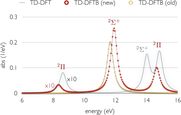
Figure 1: Absorption spectrum of nitric oxide as obtained with full TD-DFT (PBE/TZP), traditional TD-DFTB (old) and TD-DFTB with on-site corrections (new).

The electric-dipole-allowed transitions $~{}^{1}\Pi_{u}$ and $~{}^{3}\Pi_{u}$ of the homonuclear molecules N₂ and O₂ (point group D_∞h), respectively, are neither correctly described by traditional TD-DFTB as shown in 1. When applying the onsite correction, these excitations become allowed with oscillator strengths in agreement with ab-initio results. However, it is necessary to indicate that the excitation energy of the latter transition is somewhat overestimated, being in better agreement within the non-corrected formalism. In contrast, the onsite correction greatly improves the agreement of the excitation energy of N${}_{2}~{}^{1}\Pi_{u}$ with the TD-DFT result. This transition and the $~{}^{3}\Pi_{u}$ state are degenerate according to traditional results whereas such degeneracy is broken at the corrected TD-DFTB level. This degeneracy breaking is in total correspondence with the results obtained at a higher level of theory.

The original formalism also predicts the degeneracy of the singlet and triplet $\Sigma^{-}_{u}$ and $\Delta_{u}$ states of N₂ with excitation energy equal to 9.01 eV. This is however only partially confirmed by the ab-initio results and in total disagreement with the experimental findings. According to TD-DFT, the triplet and singlet $\Sigma_{u}^{-}$ states are degenerate with corresponding excitation energy of 9.60 eV but the triplet and singlet $\Delta_{u}$ degeneracy is not observed. On the other hand, experiments report nearly degenerate $\Sigma_{u}^{-}$ states with excitation energies of 9.67 and 9.92 eV for the triplet and singlet states, respectively, in contrast with TD-DFT findings. This apparent failure of TD-DFT has been also reproduced elsewhere. Grabo et al. (2000); Bauernschmitt and Ahlrichs (1996). In a recent letter it was shown that excited states like N₂ $\Sigma_{u}^{-}$ cannot be described by linear-response TD-DFT as their corresponding excitation energies do not correspond to poles of the response function Hesselmann and Goerling (2009). TD-DFTB as an approximation to TD-DFT unavoidably inherits this issue and our correction is unable to fix it. However, it does break the wrong degeneracy of the triplet and singlet $\Delta_{u}$ states. For O₂, a similar degeneracy breaking of the transitions $\Sigma_{u}^{-}$ and $\Delta_{u}$ within the corrected TD-DFTB can be observed. This is again in total agreement with first-principle results.

V.2 General benchmark

To assess the general performance of the corrected TD-DFTB method in terms of vertical excitation energies we have chosen a large benchmark set defined elsewhere Schreiber et al. (2008) and recently used for the validation of TD-DFTB Trani et al. (2011). This set covers $\pi\rightarrow\pi^{*}$, $n\rightarrow\pi^{*}$ and $\sigma\rightarrow\pi^{*}$ excitations for 28 organic compounds comprising unsaturated aliphatic hydrocarbons (group 1), aromatic hydrocarbons and heterocycles (group 2), carbonyl compounds (group 3) and nucleobases (group 4), and intends to embrace the most important chromophores in organic photochemistry. For comparison we have calculated singlet and triplet vertical excitation energies at the TD-DFT (PBE, TZP) level. To disentangle the accuracy of the TD-DFTB approximation itself from the quality of DFTB ground state geometries, the same optimized structures were used along the benchmark. These geometries were previously obtained at a MP2 level Schreiber et al. (2008). In the Supporting Information, an extended table containing all our calculation results can be consulted. For further comparison, we also provide the theoretical best estimates (TBE) for this benchmark set, calculated at the CASPT2 level and reported by Schreiber and co-workers.Schreiber et al. (2008). Reported experimental values for some vertical excitation energies are additionally given. We also include the KS energy difference of the corresponding dominant single-particle transition, which is useful for the analysis of the relative displacement of the excitation energies with respect to the KS energy difference as compared to ab-initio TD-DFT.

In 2 and 3, we present a statistical analysis of the collected data for the groups of compounds previously mentioned, for singlet-to-singlet and singlet-to-triplet transitions, respectively. In 4 the global statistics for the benchmark set is summarized. Here the analysis has been also split into triplet and singlet excitations. The mean signed difference (MSD) as well as the root-mean-square deviation (RMS) of the TD-DFTB excitation energies with respect to the experiment, the TBE and TD-DFT are reported. Statistics on ab-initio TD-DFT results are also provided to indicate its degree of correspondence with higher level of theory and experiment.

		count	TD-DFT	TD-DFTB
				$new$	$old$
Group 1
MSD	(TD-DFT)	13		0.15	0.07
	(TBE)	13	-0.52	-0.37	-0.45
	(Exp.)	12	-0.35	-0.20	-0.26
RMS	(TD-DFT)	13		0.28	0.25
	(TBE)	13	0.62	0.47	0.53
	(Exp.)	12	0.56	0.39	0.46
Group 2
MSD	(TD-DFT)	53		0.23	0.12
	(TBE)	53	-0.35	-0.12	-0.23
	(Exp.)	42	-0.06	0.13	0.02
RMS	(TD-DFT)	53		0.41	0.36
	(TBE)	53	0.54	0.37	0.43
	(Exp.)	42	0.39	0.35	0.34
Group 3
MSD	(TD-DFT)	19		0.56	0.37
	(TBE)	19	-0.81	-0.25	-0.44
	(Exp.)	13	-0.67	0.07	-0.08
RMS	(TD-DFT)	19		1.06	0.93
	(TBE)	19	0.96	0.88	0.88
	(Exp.)	13	0.88	0.70	0.64
Group 4
MSD	(TD-DFT)	19		0.09	0.03
	(TBE)	19	-0.84	-0.75	-0.81
	(Exp.)	13	-0.51	-0.37	-0.29
RMS	(TD-DFT)	19		0.32	0.30
	(TBE)	19	0.89	0.91	0.96
	(Exp.)	13	0.63	0.61	0.64

Table 2: Mean signed difference (MSD) and root-mean-square deviation (RMS) of singlet-singlet vertical excitation energies (in eV) calculated within TD-DFTB and TD-DFT (along the rows) with respect to TD-DFT, TBE and experiment (along the columns) where possible.

		count	TD-DFT	TD-DFTB
				$new$	$old$
Group 1
MSD	(TD-DFT)	13		0.21	0.71
	(TBE)	13	-0.32	-0.11	0.39
	(Exp.)	11	-0.21	0.00	0.54
RMS	(TD-DFT)	13		0.32	0.78
	(TBE)	13	0.38	0.18	0.48
	(Exp.)	11	0.25	0.21	0.61
Group 2
MSD	(TD-DFT)	36		0.28	0.55
	(TBE)	36	-0.52	-0.24	0.03
	(Exp.)	12	-0.19	0.26	0.59
RMS	(TD-DFT)	36		0.41	0.63
	(TBE)	36	0.63	0.41	0.45
	(Exp.)	12	0.33	0.38	0.69
Group 3
MSD	(TD-DFT)	14		0.42	0.79
	(TBE)	14	-0.61	-0.20	0.17
	(Exp.)	7	-0.53	-0.13	0.27
RMS	(TD-DFT)	14		0.47	0.83
	(TBE)	14	0.67	0.41	0.47
	(Exp.)	7	0.57	0.39	0.57

Table 3: Mean signed difference (MSD) and root-mean-square deviation (RMS) of singlet-triplet vertical excitation energies (in eV) calculated within TD-DFTB and TD-DFT (along the rows) with respect to TD-DFT, TBE and experiment (along the columns) where possible.

		count	TD-DFT	TD-DFTB
				$new$	$old$
Singlets
MSD	(TD-DFT)	104		0.25	0.14
	(TBE)	104	-0.55	-0.29	-0.40
	(Exp.)	80	-0.28	-0.01	-0.12
RMS	(TD-DFT)	104		0.57	0.50
	(TBE)	104	0.71	0.63	0.66
	(Exp.)	80	0.56	0.48	0.47
Triplets
MSD	(TD-DFT)	63		0.29	0.63
	(TBE)	63	-0.50	-0.20	0.14
	(Exp.)	30	-0.27	0.07	0.50
RMS	(TD-DFT)	63		0.40	0.71
	(TBE)	63	0.59	0.38	0.46
	(Exp.)	30	0.38	0.33	0.63
Total
MSD	(TD-DFT)	167		0.27	0.33
	(TBE)	167	-0.53	-0.26	-0.20
	(Exp.)	110	-0.28	0.01	0.05
RMS	(TD-DFT)	167		0.51	0.59
	(TBE)	167	0.67	0.55	0.59
	(Exp.)	110	0.52	0.44	0.52

Table 4: Global statistics for vertical excitation energies (in eV) calculated within TD-DFTB and TD-DFT (along the rows) with respect to TD-DFT, TBE and experiment (along the columns) where possible.

To assess the validity of our approximation, we focus on the comparison with the TD-DFT (PBE) data set. It is important to recall that TD-DFTB parameters are calculated at this level of theory and the main aim of our approach is to improve its agreement with respect to the TD-DFT description. Since TD-DFT at the PBE level is of course an approximation itself, we are also interested in examining the accuracy of our method compared to a higher level of theory and experiment. It is worth mentioning that the subset of singlet-triplet excitations for which experimental observations are provided is around 50% smaller than the original set, but we consider it still suitable to perform a statistical analysis. The TBEs are available for the complete benchmark set on the other hand and they are fairly close to their corresponding experimental values, with a RMS error of 0.24 eV for triplet states and 0.38 eV for singlet states. On average, both singlet and triplet TBEs are slightly overestimated (MSD = 0.15 eV and 0.20 eV, respectively) which should be taken into account in the further analysis. Consistent with earlier studies,Jacquemin et al. (2009, 2010) TD-DFT excitation energies at the PBE level appear to be somewhat underestimated with regard to experimental findings as a general trend (MSD = -0.28 eV and -0.27 eV for singlet and triplet states, respectively).

It can bee seen from 4 that with respect to TD-DFT, traditional TD-DFTB performs better for singlet-singlet than for singlet-triplet excitations. It should be pointed out however, that triplet states are in better agreement with the TBE values as it has been previously noticed Trani et al. (2011). Nevertheless, compared to the collected experimental findings, singlet states also appear to be better described. In fact, 4 shows a significant overestimation of triplet state energies compared to experiment (MSD = 0.50 eV) within traditional TD-DFTB. One of the main effects of our correction is the significant improvement of singlet-triplet excitation energies taking TD-DFT and experimental values as a reference. Within the refined formulation, the RMS error is reduced by 0.3 eV with respect to both TD-DFT and experiment. More importantly, the RMS error with respect to the latter (0.33 eV) is slightly lower than that for TD-DFT (0.38 eV). A similar accuracy for both TD-DFT and refined TD-DFTB can be seen for the first two group of compounds whereas for the third group, the agreement with experimental data is somewhat better for our method (see 3). In addition, whereas 4 still indicates some overestimation of the corrected TD-DFTB results with respect to TD-DFT, the MSD of our refined approach compared to experiment becomes very small, which shows that the corrected excitation energies are scattered around the experimental values. Specifically, in the group of aromatic hydrocarbons and heterocycles, excitation energies are overestimated whereas there is some underestimation for the carbonyl compounds. Only with regard to TBE, the refined excitation energies appear to be underestimated for every group of compounds.

In contrast to the observations for singlet-triplet transitions, the traditional TD-DFTB method is, on average, in slightly better agreement with TD-DFT. The RMS deviations of the corrected and non-corrected methods from TD-DFT are 0.57 eV and 0.50 eV, respectively. On the other hand, regarding the experimental references and the TBEs, both approaches perform with similar accuracy. The refined formalism returns overestimated excitation energies according to TD-DFT results, although with respect to experiment they are again spread around the reference values. In this case, the overestimation for the second group of compounds is compensated with the underestimation for the aliphatic hydrocarbons and the nucleobases, thus leading to an almost vanishing MSD (-0.01 eV). The results for the latter mentioned group of compounds are the least overestimated with respect to TD-DFT, with a MSD of only 0.09 eV. By contrast, the underestimation with respect to experiment is significant (MSD = -0.37 eV) and increases even more by taking the TBEs as the reference, for which the MSD amounts to -0.75 eV. For this group, the RMS error of TD-DFTB with respect to TBEs is remarkably high (0.91 eV and 0.96 eV for the corrected and non-corrected approaches, respectively). The limited agreement between the TD-DFTB excitation energies of the nucleobases and their TBE counterparts has been already pointed out by Trani and co-workers.Trani et al. (2011) However, it is necessary to notice that this failure should be rather attributed to TD-PBE itself and not to TD-DFTB as an approximation. In fact, the worst agreement between TD-DFT and TBE along the benchmark set is found for the carbonyl compounds and the nucleobases, with RMS errors of 0.96 eV and 0.89 eV, respectively. A very recent study by Foster and Wong indeed shows that conventional semi-local functionals fail in the description of the optical properties of nucleobases, while tuned range-separated functionals offer significant improvements.Foster and Wong (2012)

The overall analysis (see bottom of 4) leads to somewhat smaller RMS errors for corrected TD-DFTB compared to the non-corrected formalism. It should be indicated, that despite the important improvements for the triplets states within the corrected formulation, the benchmark set for singlet-singlet excitations is comparatively larger, conceding more importance to these kind of transitions within the total balance. As a general behavior, it can be stated that TD-DFTB singlet excited states are shifted up in energy when the onsite correction is switched on. Inversely, our correction tends to shift triplet states down. This effect is particularly noticeable for $n\rightarrow\pi^{*}$ and $\sigma\rightarrow\pi^{*}$ excitations. The excitation energies for these transitions are either identically equal or (for few cases) very close to their corresponding KS energy differences at the non-corrected TD-DFTB level, resulting in degenerate or nearly-degenerate singlet and triplet states (see Supporting Information). The only exception for this statement are the triplet $B_{1u}$ states of tetrazine, for which an energy displacement occurs also for traditional TD-DFTB, although clearly underestimated with respect to the TD-DFT results. Within the onsite correction the excitation energies are either shifted down for triplets or shifted up for singlets with respect to the KS energy difference, leading to a singlet-triplet gap in accordance with the observations at the TD-DFT level. A similar degeneracy breaking was shown earlier for N₂.

Considering only $n\rightarrow\pi^{*}$ and $\sigma\rightarrow\pi^{*}$ transitions, the RMS error of singlet-triplet excitation energies at the corrected (non-corrected) TD-DFTB level as compared to TD-DFT is 0.58 (0.82) eV. These kind of excitations are evidently difficult cases for the traditional formalism and an important improvement is obtained with the onsite correction, although the major quantitative enhancement of the latter approach is for singlet-triplet $\pi\rightarrow\pi^{*}$ transitions. Indeed, $n\rightarrow\pi^{*}$ and $\sigma\rightarrow\pi^{*}$ excitation energies are still strongly overestimated at the corrected TD-DFTB level with respect to TD-DFT, with MSD of 0.49 and 0.32 eV for triplet and singlet states, respectively. However, if we compare our findings with the TBEs, those are by contrast, significantly underestimated (MSD = -0.21 and -0.40 eV for singlet-triplet and singlet-singlet transitions, respectively) and the RMS deviations for both corrected and non-corrected formalisms are similar.

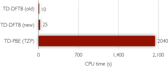
Figure 2: Total computational time required for calculating the low-lying excitation energies of a set of 28 molecules with traditional TD-DFTB (old), refined TD-DFTB (new) and full TD-DFT (PBE/TZP).

VI CONCLUSIONS

We have introduced and implemented new extensions of the time-dependent density functional based tight binding (TD-DFTB) method. By taking the formalism beyond a mere Mulliken approximation, we have been able to surpass the wrong description of $n\rightarrow\pi^{*}$ and $\sigma\rightarrow\pi^{*}$ excitations within TD-DFTB. It was shown that particularly for the molecules O₂, NO and N₂ these kind of transitions play an important role in the low energy optical spectra. Our refined formulation is in this case essential to obtain a qualitatively correct spectrum. Moreover, for the close-shell molecule N₂, the wrong $\sigma\rightarrow\pi^{*}$ triplet-singlet degeneracy encountered by using the original approach was successfully overcome. We additionally identified the erroneous degeneracy of $\pi\rightarrow\pi^{*}$ excitations with irreducible representations $\Sigma^{-}$ and $\Delta$ for the investigated diatomic molecules as another failure of traditional TD-DFTB. The new formulation now delivers the correct behavior as compared to TD-DFT observations. Along with the qualitative improvement, a better numerical agreement with TD-DFT results can also be perceived for these systems.

To extend the analysis of the performance of our correction, we calculated the low-lying vertical excitation energies for a set of 28 benchmark compounds. We found a considerable improvement in the agreement with TD-DFT and experiment in terms of singlet-triplet excitation energies, whereas singlet-singlet energies have the same overall quality as in the traditional scheme. The accuracy of the corrected formalism is similar to that of TD-DFT for both triplet and singlet states, whereas the computational time of the former method is roughly eighty times smaller (see 2).

VII ACKNOWLEDGEMENT

Financial support from the Deutsche Forschungsgemeinschaft (GRK 1570 and SPP 1243) and the DAAD is gratefully acknowledged.

Appendix A Onsite correction to the total energy

Let $\{\phi_{\alpha}\}$ and $\{\phi_{\beta}\}$ be a complete set of real orbitals placed at atom $A$ and $B$, respectively. The orbitals are assumed to be orthonormal within each set, while the overlap between orbitals on different atoms is given by $S_{\alpha\beta}$. Let also $\mu\in A$, $\nu\in B$, $\kappa\in C$ and $\lambda\in D$ unless otherwise specified. Then, the orbitals $\phi_{\mu}$ and $\phi_{\nu}$ can be expanded as

$$\phi_{\mu}(\mathbf{r})=\sum_{\beta\in B}S_{\beta\mu}\phi_{\beta}(\mathbf{r}),~{}~{}~{}\phi_{\nu}(\mathbf{r})=\sum_{\alpha\in A}S_{\alpha\nu}\phi_{\alpha}(\mathbf{r}).$$ (34)

Hence, the orbital product can be expressed as

$$\phi_{\mu}(\mathbf{r})\phi_{\nu}(\mathbf{r})=\frac{1}{2}\left(\sum_{\alpha\in A}S_{\alpha\nu}\phi_{\alpha}(\mathbf{r})\phi_{\mu}(\mathbf{r})+\sum_{\beta\in B}S_{\beta\mu}\phi_{\beta}(\mathbf{r})\phi_{\nu}(\mathbf{r})\right),$$ (35)

and more conveniently as

$$\phi_{\mu}(\mathbf{r})\phi_{\nu}(\mathbf{r})=\frac{1}{2}S_{\mu\nu}\left(|\phi_{\mu}(\mathbf{r})|^{2}+|\phi_{\nu}(\mathbf{r})|^{2}\right)+\frac{1}{2}\left(\sum_{\alpha\in A}^{\alpha\neq\mu}S_{\alpha\nu}\phi_{\alpha}(\mathbf{r})\phi_{\mu}(\mathbf{r})+\sum_{\beta\in B}^{\beta\neq\nu}S_{\beta\mu}\phi_{\beta}(\mathbf{r})\phi_{\nu}(\mathbf{r})\right),$$ (36)

where the first term accounts for the Mulliken approach. Let us now denote with $(\mu\nu|\kappa\lambda)$ a two-electron integral with an arbitrary kernel. Using 36, the integrals $(\mu\nu|\kappa\lambda)$ can then be expanded as

$$(\mu\nu|\kappa\lambda) = \frac{1}{4}S_{\mu\nu}S_{\kappa\lambda}\left[(\mu\mu|\kappa\kappa)+(\mu\mu|\lambda\lambda)+(\nu\nu|\kappa\kappa)+(\nu\nu|\lambda\lambda)\right]$$ (37)

$$+ \frac{1}{4}S_{\mu\nu}\left(\sum_{\gamma\in C}^{\gamma\neq\kappa}S_{\gamma\lambda}\left[(\mu\mu|\kappa\gamma)+(\nu\nu|\kappa\gamma)\right]+\sum_{\delta\in D}^{\delta\neq\lambda}S_{\delta\kappa}\left[(\mu\mu|\delta\lambda)+(\nu\nu|\delta\lambda)\right]\right)$$

$$+ \frac{1}{4}S_{\kappa\lambda}\left(\sum_{\alpha\in A}^{\alpha\neq\mu}S_{\alpha\nu}\left[(\mu\alpha|\kappa\kappa)+(\mu\alpha|\lambda\lambda)\right]+\sum_{\beta\in B}^{\beta\neq\nu}S_{\beta\mu}\left[(\beta\nu|\kappa\kappa)+(\beta\nu|\lambda\lambda)\right]\right)$$

$$+ \frac{1}{4}\left(\sum_{\alpha\in A}^{\alpha\neq\mu}\sum_{\gamma\in C}^{\gamma\neq\kappa}S_{\alpha\nu}S_{\gamma\lambda}(\mu\alpha|\kappa\gamma)+\sum_{\alpha\in A}^{\alpha\neq\mu}\sum_{\delta\in D}^{\delta\neq\lambda}S_{\alpha\nu}S_{\delta\kappa}(\mu\alpha|\delta\lambda)\right)$$

$$+ \frac{1}{4}\left(\sum_{\beta\in B}^{\beta\neq\nu}\sum_{\gamma\in C}^{\gamma\neq\kappa}S_{\beta\mu}S_{\gamma\lambda}(\beta\nu|\kappa\gamma)+\sum_{\beta\in B}^{\beta\neq\nu}\sum_{\delta\in D}^{\delta\neq\lambda}S_{\beta\mu}S_{\delta\kappa}(\beta\nu|\delta\lambda)\right).$$

Note that the expression 37 is exact as long as the AO sets $\{\phi_{\alpha}\}$, $\{\phi_{\beta}\}$, $\{\phi_{\gamma}\}$ and $\{\phi_{\delta}\}$ are complete. The first line in eq 37 contains the leading terms, which include Coulomb-like integrals. Truncation of the expansion up to the first line accounts for the Mulliken approach. A next level of approximation demands the inclusion of fully-onsite exchange-like integrals, i.e. $(\mu\nu|\mu\nu)$, with $\mu,\nu\in A$ and $\mu\neq\nu$. At this level of theory the general four-center integrals can be expressed as

$$(\mu\nu|\kappa\lambda)\approx(\mu\nu|\kappa\lambda)_{\text{mull}}+(\mu\nu|\kappa\lambda)_{\text{ons}},$$ (38)

where

$$(\mu\nu|\kappa\lambda)_{\text{mull}}=\frac{1}{4}S_{\mu\nu}S_{\kappa\lambda}\left[(\mu\mu|\kappa\kappa)+(\mu\mu|\lambda\lambda)+(\nu\nu|\kappa\kappa)+(\nu\nu|\lambda\lambda)\right],$$ (39)

and

$$(\mu\nu|\kappa\lambda)_{\text{ons}} = \frac{1}{4}\sum_{\alpha\in A}^{\alpha\neq\mu}S_{\alpha\nu}S_{\alpha\lambda}(\mu\alpha|\mu\alpha)\delta_{\mu\kappa}+\frac{1}{4}\sum_{\alpha\in A}^{\alpha\neq\mu}S_{\alpha\nu}S_{\alpha\kappa}(\mu\alpha|\mu\alpha)\delta_{\mu\lambda}$$ (40)

$$+ \frac{1}{4}\sum_{\beta\in B}^{\beta\neq\nu}S_{\beta\mu}S_{\beta\lambda}(\beta\nu|\beta\nu)\delta_{\nu\kappa}+\frac{1}{4}\sum_{\beta\in B}^{\beta\neq\nu}S_{\beta\mu}S_{\beta\kappa}(\beta\nu|\beta\nu)\delta_{\nu\lambda}$$

$$+ \frac{1}{4}S_{\kappa\nu}S_{\mu\lambda}(\mu\kappa|\mu\kappa)\delta_{AC}(1-\delta_{\mu\kappa})+\frac{1}{4}S_{\lambda\nu}S_{\mu\kappa}(\mu\lambda|\mu\lambda)\delta_{AD}(1-\delta_{\mu\lambda})$$

$$+ \frac{1}{4}S_{\kappa\mu}S_{\nu\lambda}(\nu\kappa|\nu\kappa)\delta_{BC}(1-\delta_{\nu\kappa})+\frac{1}{4}S_{\lambda\mu}S_{\nu\kappa}(\nu\lambda|\nu\lambda)\delta_{BD}(1-\delta_{\nu\lambda})\,.$$

The contribution to the DFTB total energy originating from this correction is written as

$$E_{\text{ons}}=\frac{1}{2}\sum_{\sigma\tau}\sum_{\mu\nu\kappa\lambda}\Delta P_{\mu\nu}^{\sigma}\left(\mu\nu|f^{\text{hxc}}_{\rho_{\sigma}\rho_{\tau}}[\rho_{0}]|\kappa\lambda\right)_{\text{ons}}\,\Delta P_{\kappa\lambda}^{\tau}.$$ (41)

After substituting 40 in 41, we finally arrive at

$$E_{\text{ons}}=\sum_{\sigma\tau}\sum_{A}\sum_{\mu\nu\in A}^{\mu\neq\nu}\Delta\tilde{P}_{\mu\nu}^{\sigma}\left(\mu\nu|f^{\text{hxc}}_{\rho_{\sigma}\rho_{\tau}}[\rho_{0}]|\mu\nu\right)\Delta\tilde{P}_{\mu\nu}^{\tau},$$ (42)

where $\tilde{P}_{\mu\nu}^{\sigma}$ are the matrix elements of the dual density matrix defined in 8.

Appendix B Onsite correction to dipole matrix elements

To derive an expression for the KS dipole matrix elements, we expand the KS orbitals into a set of localized atom-centered AO, $\psi_{s\sigma}=\sum_{\mu}c_{\mu s}^{\sigma}\phi_{\mu}$. Thus, the dipole matrix elements read

$$\langle\psi_{s\sigma}|\mathbf{\hat{r}}|\psi_{t\sigma}\rangle=\sum_{\mu\nu}c_{\mu s}^{\sigma}\langle\mu|\mathbf{\hat{r}}|\nu\rangle c_{\nu t}^{\sigma}$$ (43)

Let $\mu\in A$ and $\nu\in B$ unless otherwise indicated. Using the orbital product expansion 36, the AO dipole matrix elements, $\langle\mu|\mathbf{\hat{r}}|\nu\rangle$, can be expressed as follows,

$$\langle\mu|\mathbf{\hat{r}}|\nu\rangle=\frac{1}{2}S_{\mu\nu}\left(\mathbf{R}_{A}+\mathbf{R}_{B}\right)+\frac{1}{2}\left(\sum_{\alpha\in A}^{\alpha\neq\mu}S_{\alpha\nu}\langle\alpha|\mathbf{\hat{r}}|\mu\rangle+\sum_{\beta\in B}^{\beta\neq\nu}S_{\beta\mu}\langle\beta|\mathbf{\hat{r}}|\nu\rangle\right),$$ (44)

where $\mathbf{R}_{A}=\langle\mu|\mathbf{\hat{r}}|\mu\rangle$ and $\mathbf{R}_{B}=\langle\nu|\mathbf{\hat{r}}|\nu\rangle$ denote the positions of centers A and B, respectively. After substituting 44 in 43, we finally have

$$\langle\psi_{s\sigma}|\mathbf{\hat{r}}|\psi_{t\sigma}\rangle=\sum_{A}\mathbf{R}_{A}q_{A}^{st\sigma}+\sum_{A}\sum_{\mu\nu\in A}^{\mu\neq\nu}P_{\mu\nu}^{st\sigma}\langle\mu|\mathbf{\hat{r}}|\nu\rangle,$$ (45)

where the definition 10 was additionally employed.

References

- Runge and Gross (1984) Runge, E.; Gross, E. K. U. Phys. Rev. Lett. 1984, 52, 997–1000.
- Casida and Huix-Rotllant (2012) Casida, M. E.; Huix-Rotllant, M. Annu. Rev. Phys. Chem. 2012, 63, 287.
- Niehaus et al. (2001) Niehaus, T. A.; Suhai, S.; Della Sala, F.; Lugli, P.; Elstner, M.; Seifert, G.; Frauenheim, T. Phys. Rev. B 2001, 63, 085108.
- Heringer et al. (2007) Heringer, D.; Niehaus, T. A.; Wanko, M.; Frauenheim, T. J. Comp. Chem. 2007, 28, 2589–601.
- Yam et al. (2003) Yam, C. Y.; Yokojima, S.; Chen, G. H. Physical Review B 2003, 68, 153105.
- Niehaus et al. (2005) Niehaus, T. A.; Heringer, D.; Torralva, B.; Frauenheim, T. Eur. Phys. J. D 2005, 35, 467–477.
- Mitric et al. (2009) Mitric, R.; Werner, U.; Wohlgemuth, M.; Seifert, G.; Bonacic-Kouteckỳ, V. J. Phys. Chem. A 2009, 113, 12700.
- Jakowski et al. (2012) Jakowski, J.; Irle, S.; Morokuma, K. Phys. Chem. Chem. Phys. 2012, 14, 6273.
- Wang et al. (2011) Wang, Y.; Yam, C.-Y.; Frauenheim, T.; Chen, G.; Niehaus, T. Chem. Phys. 2011, 391, 69, ¡ce:title¿Open problems and new solutions in time dependent density functional theory¡/ce:title¿.
- Trani et al. (2011) Trani, F.; Scalmani, G.; Zheng, G.; Carnimeo, I.; Frisch, M.; Barone, V. J. Chem. Theory Comput. 2011, 7, 3304.
- Niehaus (2009) Niehaus, T. A. J. Mol. Struct.: THEOCHEM 2009, 914, 38.
- Köhler et al. (2001) Köhler, C.; Seifert, G.; Gerstmann, U.; Elstner, M.; Overhof, H.; Frauenheim, T. Phys. Chem. Chem. Phys. 2001, 3, 5109–5114.
- Frauenheim et al. (2002) Frauenheim, T.; Seifert, G.; Elstner, M.; Niehaus, T.; Kohler, C.; Amkreutz, M.; Sternberg, M.; Hajnal, Z.; Di Carlo, A.; Suhai, S. Journal Of Physics-Condensed Matter 2002, 14, 3015–3047.
- Casida (1995) Casida, M. E. In Recent Advances in Density Functional Methods, Part I; Chong, D., Ed.; World Scientific, 1995; Chapter Time-dependent Density Functional Response Theory for Molecules, pp 155–192.
- Niehaus and Della Sala (2012) Niehaus, T.; Della Sala, F. physica status solidi (b) 2012, 249, 237.
- Pople et al. (1967) Pople, J. A.; Beveridge, D. L.; Dobosh, P. A. J. Chem. Phys. 1967, 47, 2026.
- Pople et al. (1965) Pople, J. A.; Santry, D. P.; Segal, G. A. J. Phys. Chem. 1965, 43, S129.
- Figeys et al. (1977) Figeys, H.; Geerlings, P.; Van Alsenoy, C. Int. J. Quantum Chem. 1977, 11, 705–713.
- Perdew et al. (1996) Perdew, J.; Burke, K.; Ernzerhof, M. Phys. Rev. Lett. 1996, 77, 3865–3868.
- Elstner et al. (1998) Elstner, M.; Porezag, D.; Jungnickel, G.; Elsner, J.; Haugk, M.; Frauenheim, T.; Suhai, S.; Seifert, G. Phys. Rev. B 1998, 58, 7260–7268.
- Niehaus et al. (2001) Niehaus, T. A.; Elstner, M.; Frauenheim, T.; Suhai, S. J. Mol. Struct. - Theochem 2001, 541, 185–194.
- Aradi et al. (2007) Aradi, B.; Hourahine, B.; Frauenheim, T. J. Phys. Chem. A 2007, 111, 5678–5684.
- Maurice and Head-Gordon (1995) Maurice, D.; Head-Gordon, M. Int. J. Quantum Chem. Symp. 1995, 29, 361.
-
(24)
TURBOMOLE V6.4 2012, a development of University of Karlsruhe and
Forschungszentrum Karlsruhe GmbH, 1989-2007, TURBOMOLE GmbH, since 2007;
available from
http://www.turbomole.com. - Oddershede et al. (1985) Oddershede, J.; Gruener, N. E.; Diercksen, G. H. F. Chem. Phys. 1985, 97, 303.
- Krupenie (1972) Krupenie, P. H. J. Phys. Chem. Ref. Data 1972, 1(2), 423.
- Grabo et al. (2000) Grabo, T.; Petersilka, M.; Gross, E. K. U. J. Mol. Struc.-THEOCHEM 2000, 501-502, 353.
- Bauernschmitt and Ahlrichs (1996) Bauernschmitt, R.; Ahlrichs, R. Chem. Phys. Lett. 1996, 256, 454.
- Hesselmann and Goerling (2009) Hesselmann, A.; Goerling, A. Phys. Rev. Lett. 2009, 102, 233003.
- Schreiber et al. (2008) Schreiber, M.; Silva-Junior, M.; Sauer, S.; Thiel, W. J. Chem. Phys. 2008, 128, 134110.
- Jacquemin et al. (2009) Jacquemin, D.; Wathelet, V.; Perpete, E. A.; Adamo, C. J. Chem. Theory Comput. 2009, 5, 2420–2435.
- Jacquemin et al. (2010) Jacquemin, D.; Perpete, E. A.; Ciofini, I.; Adamo, C. J. Chem. Theory Comput. 2010, 6, 1532–1537.
- Foster and Wong (2012) Foster, M. E.; Wong, B. M. J. Chem. Theory Comput. 2012, 8, 2682–2687.