DEMONic Dominoes
Measuring the Speed of the Domino Effect from Sound Recordings

Abstract.

In response to a challenge in a recent paper to measure the propagation speed of the wave of collapse of an array of dominoes (the Domino Effect), a novel method of measuring the speed of such waves has been developed using sound recordings of the collapse and DEMON (Detection of Modulation on Noise) analysis to extract the frequency of domino impacts and hence the speed of propagation of the domino wave. This paper presents this method and a discussion of the other published measurements and models and some comments on the precess of mathematical modelling.

1. Introduction

Recent interest in the speed of propagation of the domino effect seems to originate with a question by Daykin [1] in the problems section of SCIAM review, and the initial response from McLachlan and Beaupre [7] where they presented a dimensional analysis of the wave speed and some experimental results. Subsequently a number of authors have presented mathematical models of the propagation of domino waves of varying levels of detail and complexity (a partial list includes [2] [3] [4] [5] [6] [8]). Also there have been additional measurements reported [3] [4] (which may also be found in [5])

In a recent paper on the modelling of the propagation speed of domino waves [2] a challenge was thrown down to actually measure the speed. This seemed an interesting problem, and my initial thoughts were of videoing the collapse of a domino array using a digital camera(a prime consideration was that the experiment should have near zero impact on my household finances so where possible use should be made of equipment that I already owned or cost very little). After a start had been made on collecting materials for the experiment and conducting some preliminary trials with the dominoes, it occurred to me that the noise of the domino wave should encode the frequency of dominoes impacting one another, and hence the speed of the wave. As I has an old laptop computer with a sound recorder built in and a spare computer microphone, recording the sound would entail zero equipment cost, and would be less fiddly than videoing (extracting and analysing the frames of a video is very time consuming, I know because I have used the technique before when looking at the kinematics of bouncing).

All the results reported here used the same set/s of dominoes, their dimensions are given in Section 5 .

What this paper does is demonstrate the application of some interesting techniques of signal processing, some ideas from mathematical modelling and in particular the need for model validation (that is the comparison of model prediction with real data on the phenomena modelled to demonstrate that at least for such cases the model is in acceptable agreement with the model)

2. Dimensional Theory

McLachlan et al. [7] conclude from dimensional analysis that the limiting wave speed $V$ for thin dominoes satisfies:

$$\frac{v}{\sqrt{gH}}=G(L/H)$$

for some function $G$. Which for thin dominoes is the same as:

$$\frac{v}{\sqrt{gH}}=G_{1}(d/H)$$

Where $H$ is the height of the dominoes, $d$ the gap between adjacent dominoes, and $L$ the distance between equivalent points on neighbouring dominoes (that is the pitch of the domino array) (see figure 1 for the significance of the variables). McLachlan et al. do not give their analysis that leads to these results, but it is easy enough to reconstruct.

Notes: There are additional dimensionless parameters hidden in functions $G$ and $G_{1}$ as the normalised speed also depend on the dimensionless constants characteristic of the materials involved, in this case these include the coefficient of friction between dominoes, and the coefficient of restitution for inter domino impacts. The coefficient of friction between the surface and the dominoes is of lesser relevance as in domino experiments it is usual to arrange things so that there is no slipping between the dominoes and the surface. The models in Stonge [3], Strong and Shu [4] and Van Leeuwen [6] represent the effects of these, but as the experimental results show the material properties of the dominoes for the materials tested have a minor influence on the wave speed.

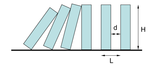
Figure 1. Geometry of Domino Array

3. Data Generation and Collection

Initially I had toyed with the idea of videoing domino waves, then extracting the speed from an analysis of the video’s frames. I abandoned this approach when I realised that audio recording would be more convenient. The way that I decided to measure the domino wave speed was to use the sound recorder and microphone on an old laptop to record the sound of a domino array collapse. (This is far less demanding in terms of cost of equipment than the high speed photography reported in [3], [4] and [5]). Then to analyse the recording to extract the frequency of dominoes hitting the their adjacent domino (which is a simpler process than manually analysing frames of a video).

The experimental set up is shown in figure 2 (in any future experiments the computer will be moved away from the rest of the set up as in retrospect it seems that the computer fan was probably the limiting noise source for the experiments).

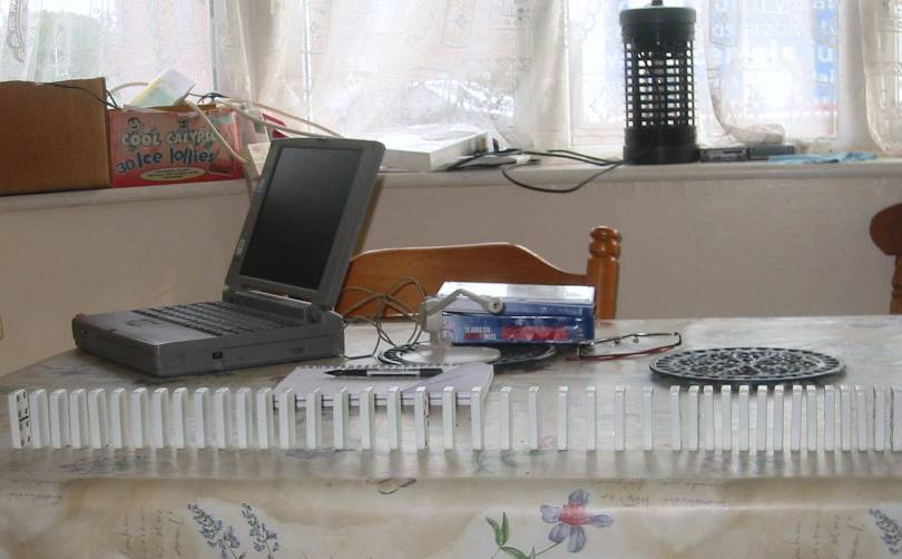
Figure 2. Photo of Experimental Set Up for an Early Pilot Run

The signal of interest is encoded in the envelope of the recording so analysis techniques analogous to the processing in a crystal AM radio receiver, or a simple form of DEMON (Detection of Envelope Modulation On Noise) analysis similar to that used in passive Sonar processing is required (unclassified references for DEMON, other than publicity releases for equipment that uses it, are difficult to find but Kummert [9] includes a description). The initial sections of each recording were progressively discarded to identify and eliminate any start up transients. For most of the recordings the transients were at most slight and easily eliminated, but four must be regarded with caution (the two with the closest and the two with the widest relatively spacing of the dominoes) as the results for these were inconsistent (they could be repeated more carefully).

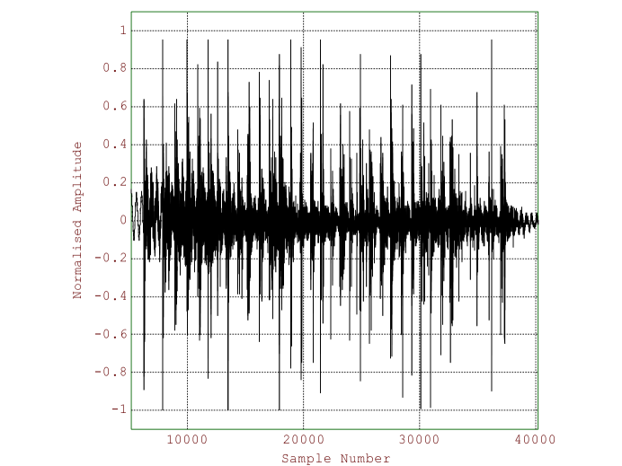
Figure 3. Plot of the Sound Recording of a Domino Wave

4. Processing of Acoustic Data

The Windows sound recorder produces a .wav file as its output which contains the recorded data. This (in our case) was sampled at $\sim 22$ kHz (about 22000 samples per second) with 1 byte (8 bits) per sample, which in principle gives $2^{8}\ (256)$ different levels. For analysis the data is shifted to have zero mean and normalised to the range $(-1,1)$.

There are several artefacts in the recordings due to the way the sound recorder operates, and the lack of controls on the version used. The most conspicuous artefact is the result of the recorder’s Automatic Gain Control (AGC) which leads to the general decay amplitude visible in figure 3 (The plots shown in figures 3 - 6 are for a domino array with $d/H=0.62$). Also just visible in figure 3 is the zero offset in the short segment of data visible before the sound of the dominoes starts to dominate. For the analyses that are applied to the data these artefacts are of little to no importance, effectively introducing additional “noise” which we will see is not a real problem.

Looking at figure 3 or the plot of the rectified data shown in figure 4 we see a series of spikes that look as though they are near periodic, these are predominantly the clicks of the dominoes hitting one another. It is the average frequency of occurrence of these clicks together with the nominal domino spacing that allows us to deduce the speed of the domino wave.

In order to extract the “average” frequency of the spikes we perform a frequency analysis of the rectified waveform shown figure 4. We use the rectified data for this because the spectrum of the unrectified data shows no obvious features at the spike frequency, the dominant low frequency feature is hum at around 50 Hz. The spike frequency if present will appear as a modulating frequency on tones (of phase random from spike to spike) or on noise. If we look at the full spectrum our suspicion that there will be no features that are easily identifiable as such are confirmed. Figure 5 shows the low frequency part of the spectrum of the rectified signal. Here we see a large spike at zero frequency due to the positivity of the signal, the next peak at $\sim 25$ Hz is the frequency we seek, there are also faint signs of harmonics of this frequency (these are more obvious in equivalent plots for some of the other domino spacings). We also see that the hum (which should now appear at $\sim 100$ Hz) is small compared to the feature of interest. That the feature identified in figure 5 corresponds to the spike spacing in figure 4 can be shown by measuring the spacing of the spikes in figure 4.

The use of the FFT algorithm to perform the required frequency analysis is discussed in Appendix A.

The above explains the main ideas of our analysis, but to make the feature of interest clearer we filter to a band that includes the majority of the energy in the spikes and also filter out the low frequency components below $\sim 10$ Hz after rectification. This gives us the much clearer signature shown in figure 6. It is these plots of the processed data that I use to take measurements from. The data in this paper was extracted from such plots essentially by measuring semi-manually from such plots. This could be automated, and the centroid of the peaks computed rather than manually measuring the position of the tip of the peak, but I have not done that for this paper.

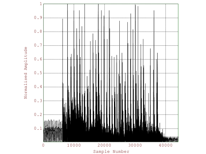
Figure 4. Plot of Rectified Recording of Domino Wave

5. Results

The experiments were all conducted with dominoes of dimensions $\approx 0.0516\times 0.0255\times 0.0079$ meters. The results shown in table 1 are for dominoes with a vertical orientation (standing on their smallest faces), and those in table 2 are for dominoes with a horizontal orientation (standing on their second smallest face).

Table 1. Experimental Results With Dominoes Vertical (italic script indicates less reliable data)

$d/H$	0.04	0.14	0.23	0.33	0.43	0.53	0.62	0.72	0.82
$V/\sqrt{gH}$	1.07	1.33	1.53	1.51	1.47	1.50	1.40	1.33	1.23

Table 2. Experimental Results With Dominoes Horizontal (italic script indicates less reliable data)

$d/H$	0.28	0.47	0.67	0.87
$V/\sqrt{gH}$	1.15	1.19	1.15	0.68

Notes The last entry in table 2 has a spacing greater than the maximum for which one would expect the domino wave to propagate. At a value of $d/H>\sqrt{3}/2$ a domino strikes its neighbour below its’ mid point, and under these conditions it may well not topple in the expected manner, this is van Leeuwen’s practical upper limit for the wave to propagate. So it is no surprise that the data for this point is unreliable and this was the largest spacing at which I could get the wave to propagate. Presumably it did propagate in this case as a result of the irregularities in the domino geometry and spacing, or some other unidentified reason.

All of the papers that report domino wave speed measurements report speeds $\sim 0.9$ to $1.7\times\sqrt{gH}$. These are in broad agreement with my own measurements, my and other published measurements are shown in figure 7.

As the results shown in table 2 are systematically lower that those in table 1 so we may suspect that one or more assumptions underlying the dimensional analysis are invalid.

Given the usual shapes of dominoes I would hope that the thin domino approximation would be not unreasonable down to values of $d/H\sim 0.2$.

As can also be seen in figure 8 the measured data are comparable to the predictions of [2] over a rather limited range of $d/H$. This is in contradistinction to the models the predictions of Bank’s [8] which in general give rather better agreement with experiment. The models which represent the effects of multiple dominoes being involved in the collapse wave being rather better than Bank’s model. Even so the reasonable agreement between the experimental data and the model predictions from Banks [8] is worth noting as it indicates that the single neighbour domino interaction assumption is not entirely misleading.

The spectral features corresponding to the wave speeds are often split into two or three closely spaced features (typically a few Hertz apart). This may be due to irregularities of the surface used for the experiments, or to some irregularity in the dominoes. When checked with a spirit level the table surface appears to be flat, but close examination of the dominoes seems to indicate that opposite short edges are not parallel. The irregularity in the dominoes appears to be substantially the same for all the dominoes, and so may be responsible for the splitting of the spectral features.

To gain some idea of the errors associated with the better data points the domino wave speed was measured multiple times for one value of domino spacing and the mean and standard deviation or the wave speed computed. This give the result that for $d/H=0.62$ we have a mean non-dimensional wave speed $V/\sqrt{gH}$ of $1.37$ with standard deviation estimated from the sample of $\sim 0.07$.

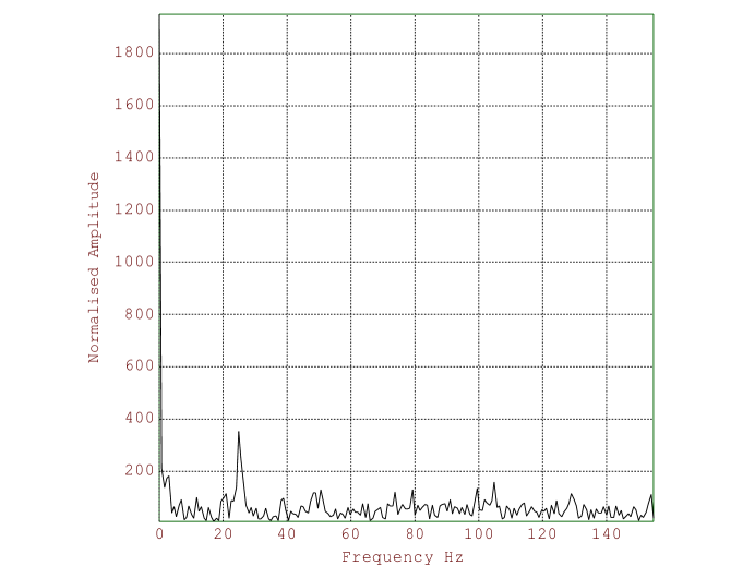
Figure 5. DEMON Amplitude Spectrum of Signal

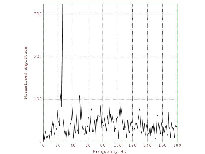
Figure 6. Processed DEMON Amplitude Spectrum of Signal

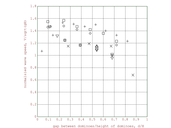
Figure 7. Domino Wave Speed Data; $+$ measurements by the current author with the dominoes vertical, $\times$ with them horizontal, $\square$ and $\lozenge$ measurements from Strong and Shu [4], $\triangledown$ (normal dominoes) and $\vartriangle$ (double height dominoes) measurements from McLachlan et al. [7]

6. Discussion

The experimental data may be summarised as telling us that to a fair (hand-waving) approximation for common dominoes the normalised wave speed is a relatively weak function of the normalised inter domino interval for practical intervals (or at most shows a slight downward trend with increasing domino spacing). Also that the normalised wave speed is of the $\sim 1$.

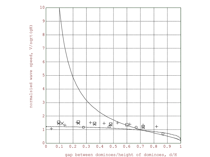
Figure 8. Domino Wave Speed Plot; the solid line is the model prediction from Efthimiou and Johnson [2], dashed line from Banks [8], $+$ measurements by the current author with the dominoes vertical, $\circ$ with them horizontal, $\times$ and $\Box$ measurements from Strong and Shu [4]

From figure 7 we can see that all the reliable data points measured in this study give normalised wave speeds in the range $\sim 1-1.6$ which is in reasonable agreement with other measurements.

It could be interesting to do some further work to improve the measurements for closely spaced dominoes with $d/H\sim 0.05-0.2$ as the current data is poor here but may with more careful work be capable of improvement. This would be interesting even if only to see how far the technique can be pushed. It would also be worthwhile to see if the quality of all the data can be improved by being careful to arrange for all the dominoes to have the best orientation.

7. Summary

From the comparison of the model of Efthimiou and Johnson [2] and experiment we see that the area of agreement of experiment and model is rather limited. Had the model been part of a project with some economic impact we would have been at risk of being found to not have shown due diligence, which could result in unfavourable consequences for us and/or our employers in the event of a failure.

Validation of models is not a chore that we may do after the interesting parts of a study are completed but an essential activity if our work is not to be nugatory.

It is also worth while comparing the predictions in the literature with ones current models predictions, the differences may be important and in need of explanation

Appendix A The Fast Fourier Transform and Frequency Analysis

When doing a frequency analysis we want to look for significant frequencies in the given signal. To do this we look at the frequency spectrum of the signal which is the square absolute value or just the absolute value (or amplitude) of the Fourier Transform (FT) of the signal. The FT breaks our signal $x(t)$ down into a linear combination of sinusoidal components, where the component at frequency $f$ is given by:

$$X(f)=\mathfrak{F}x|_{f}=\kappa\int_{-\infty}^{\infty}x(t)e^{-i(2\pi ft)}\ dt\ \ \ ...(1)$$

where $\kappa$ is a normalising factor the value of which I will not worry about as every area of application of the FT uses a different convention for normalising factors. Also the negative sign in the exponential term may in some versions of the FT be a positive sign, but none of this matters for what I am going to do, also at some point I will use library software and I don’t want to have to worry about the conventions in use, if necessary I will normalise the spectrum to have the same energy as the signal (that is the normalisation will make the integrals of their square magnitudes equal) . There is an additional ambiguity in the definition of the FT and that is over the use of angular frequency $\omega$ or plain frequency $f$, for now I will stick with $f$.

Now because we have a finite recording of the signals of interest the range of integration may be reduced to a finite interval which contains the recording:

$$X(f)=\mathfrak{F}x|_{f}=\kappa\int_{a}^{b}x(t)e^{-i(2\pi ft)}\ dt\ \ \ ...(2)$$

which is now equivalent to the computation of the coefficients of a Fourier Series and all the information in $X(f)$ is contained in $X(n/(b-a)),\ n=0,\ \pm 1,\ \pm 2...$ (in fact since $x(t)$ is a real signal $X(f)$ has complex conjugate symmetry and so everything about $x(t)$ is encoded in $X(n/(b-a)),\ n=0,\ +1,\ +2,\ ...$)

There are several problems with $(2)$ but the main one is that while the actual signal of interest is a function of the continuous time variable $t$ we only know its value at discrete sample points. To get around this problem we can use a numerical integration scheme to compute the Fourier coefficients. The scheme that I adopt is the simplest so I approximate:

$$X(k/(b-a))\approx\kappa\sum_{k}x(t_{k})\Delta te^{-i(2\pi nt_{k}/(b-a))}\ \ \ ...(3)$$

where $t_{k}=a+k\Delta t,\ \ k=0,\ ...,\ \lfloor(b-a)/\Delta t\rfloor$ which with a bit of jiggery pokery will allow the use of Fast Fourier Transform (FFT) algorithms to do our computations (for simplicity we will generally work with $b-a$ being an integer multiple of $\Delta t$). This is a desirable result because of the almost incredible efficiency of FFT algorithms. This approach is known to work well if the signal has negligible energy at frequencies above half the sampling rate (Nyquist frequency or rate) used, which is usually the case as the recording hardware will generally filter the signal to the required band before sampling.

Appendix B Data Analysis Software

The data analysis package used to to the processing described in this note was Euler Math Toolbox (EuMathT) (or rather my version of an earlier incarnation simply called Euler) This required minor modifications to the function for reading wav files to correct for a difference in the file format produced by the recorder and that expected by the function, the current version of EuMathT may have fixed this problem. In addition to the built in facilities of the data analysis package additional code to do the specific analysis and plotting required is written in the packages own BASIC like matrix language.

Alternatives to EuMathT exist and any of them would be an equally suitable tool for this job. The obvious commercial alternative is Matlab, with other freeware or Open Source packages being: SciLab, FreeMat, Octave (which to a greater of lesser extent use syntax compatible with Matlab) and Yorick. Some of the alternatives may need tweaking to get them to read wav files, but generally if the package does not have this facility built in code to implement it can usually be downloaded from the Internet. A simple search with your favourite Internet search engine will turn up links to the websites for all of these packages.

References

- [1] D. E. Daykin, Falling Dominoes, Problem 71-19 SIAM Review 17 (1971)569
- [2] C. J. Efthimiou, M. D. Johnson, Domino Waves, SIAM Review 49 (2007) 111-120.
- [3] W. J. Stronge, The domino effect: a wave of destabilizing collisions in a periodic array, Proc R. Soc Lond. A 409 (1987), 199-208
- [4] W. J. Stronge, D. Shu, The Domino Effect: Successive Destabilisation by Cooperative Neighbours, Proc R. Soc Lond. A 418 (1988), 155-163
- [5] W. J. Stronge, Impact Mechanics, Cambridge University Press 2004.
- [6] J. M. J van Leeuwen, The Domino Effect, arXiv:physics/0401018v1 (2004)
- [7] B. G. McLachlan, G. Beaupre, A. B. Cox, L. Gore, SIAM Review 25 (1983) 403-404
- [8] R. B. Banks, Towing Icebergs, Falling Dominoes, and Other Adventures in Applied Mathematics, Princeton University Press 1998.
- [9] A. Kummert, Fuzzy technology implemented in sonar systems, IEEE Journal of Oceanic Engineering 18 (1993), 483-490. (Also available at: http://www.fuzzytech.com/e/e_a_kumm.html )