Asymptotic power of likelihood ratio tests for high dimensional data

Abstract

This paper considers the asymptotic power of likelihood ratio test (LRT) for the identity test when the dimension $p$ is large compared to the sample size $n$. The asymptotic distribution of LRT under alternatives is given and an explicit expression of the power is derived when $\rm{tr}(\Sigma_{p})-\log|\Sigma_{p}|-p$ tends to a constant. A simulation study is carried out to compare LRT with other tests. All these studies show that LRT is a powerful test to detect eigenvalues around zero.

Key words and phrases: Covariance matrix, High dimensional data, Identity test, Likelihood ratio test, Power

1 Introduction

In multivariate analysis for high dimensional data, testing the structure of population covariance matrices is an important problem. See, for example, Johnstone (2001), Ledoit and Wolf (2002), Srivastava (2005), Schott (2006), Chen et al. (2010), Cai and Jiang (2011) and Li and Chen (2012), among many others. Let $X_{1},\cdots,X_{n}$ be $n$ independent and identically distributed (i.i.d.) $p$-variate random vectors following a multivariate normal distribution $N_{p}(\mu,\Sigma_{p})$ where $\mu$ is the mean vector and $\Sigma_{p}$ is the covariance matrix. In many studies, a hypothesis test of significant interest is to test

$$H_{0}:~{}\Sigma_{p}=I_{p}~{}~{}vs~{}~{}H_{1}:~{}\Sigma_{p}\neq I_{p},$$ (1)

where $I_{p}$ is the $p$-dimensional identity matrix. Note that the identity matrix in (1) can be replaced by any other positive definite matrix $\Sigma_{0}$ through multiplying the data by $\Sigma_{0}^{-1/2}$.

A natural approach to test (1) is to conduct estimations for some distance measures between $\Sigma_{p}$ and $I_{p}$ and there are two types of measures which are widely used in literature. The first is based on the likelihood function:

$$L_{l}(\Sigma_{p})=\rm{tr}(\Sigma_{p})-\log{|\Sigma_{p}|}-p,$$ (2)

and the second is based on quadratic loss function:

$$L_{q}(\Sigma_{p})=\rm{tr}(\Sigma_{p}-I_{p})^{2}.$$ (3)

Each of these is 0 when $\Sigma_{p}=I_{p}$ and positive when $\Sigma_{p}\neq I_{p}$. For $L_{l}(\Sigma_{p})$, it is referred to the likelihood ratio test (LRT) and the classic LRT for fixed $p$ and large $n$ can be found in Anderson (2003). For high dimensional data ($p$ is large), the failure of classical LRT was firstly observed by Dempster (1958) and later in a pioneer work by Bai et al. (2009), authors proposed corrections to LRT when $p/n\to c\in(0,1)$ and $\mu=0$. Successive works included Jiang et al. (2012) which extended the results of Bai et al. (2009) to Gaussian data with general $\mu$ and our work Wang et al. (2012) where we studied the LRT for general $\mu$ and non-Gaussian data. For the quadratic loss function $L_{q}(\Sigma_{p})$, there are many works since the seminal paper Nagao (1973). These included Ledoit and Wolf (2002), Birke and Dette (2005), Srivastava (2005), Chen et al. (2010) and Cai and Ma (2012). Other works which considered question (1) are referred to Johnstone (2001), Cai and Jiang (2011) and Onatski et al. (2011).

The existing results about LRT (Bai et al., 2009; Jiang et al., 2012; Wang et al., 2012) have only derived asymptotic null distribution and we know little about the asymptotic point-wise power of LRT under the alternative hypothesis. Recently, Onatski et al. (2011) studied the asymptotic power of several tests including LRT under the special alternative of rank one perturbation to the identity matrix as both $p$ and $n$ go to infinity. Cai and Ma (2012) investigated the testing problem (1) in the high-dimensional settings from a minimax point of view. The results in Onatski et al. (2011) and Cai and Ma (2012) showed that LRT was a sub-optimal test when there was a rank one perturbation to the identity matrix .

In this work, we will consider the power of LRT under general alternatives. The asymptotic distribution of LRT will be studied when $\Sigma_{p}\neq I_{p}$ and an explicit expression of the power will also be derived when $L_{l}(\Sigma_{p})$ tends to a constant. From these results, we find that in relation to LRT it is not fair that Onatski et al. (2011) and Cai and Ma (2012) only focused on the alternatives whose eigenvalues were larger than 1. Furthermore, our results show that LRT is powerful to detect eigenvalues around zero. Simulations will also be conducted to compare LRT with two tests based on $L_{q}(\Sigma_{p})$ (Chen et al., 2010; Cai and Ma, 2012).

The paper is structured as follows: Section 2 introduces the basic data structure and establishes the asymptotic power of LRT while Section 3 reports simulation studies. All the proofs are presented in the Appendix.

2 Main Results

To relax the Gaussian assumptions, we assume that the observations $X_{1},\cdots,X_{n}$ satisfy a multivariate model (Chen et al., 2010)

$$X_{i}=\Sigma_{p}^{1/2}Y_{i}+\mu,~{}for~{}i=1,\cdots,n$$ (4)

where $\mu$ is a $p$-dimensional constant vector and the entries of $\mathcal{Y}_{n}=(Y_{ij})_{p\times n}=(Y_{1},\cdots,Y_{n})$ are i.i.d. with $EY_{ij}=0$, $EY^{2}_{ij}=1$ and $EY^{4}_{ij}=3+\Delta$. The sample covariance matrix is defined as

$$S_{n}=\frac{1}{n-1}\sum_{k=1}^{n}(X_{k}-\bar{X})(X_{k}-\bar{X})^{\prime},$$

where $\bar{X}=\frac{1}{n}\sum_{k=1}^{n}X_{k}$.

Writing $y_{n}=p/n<1$, the LRT statistic is defined as

$$L_{n}=\frac{1}{p}\rm{tr}(S_{n})-\frac{1}{p}\log{|S_{n}|}-1-d(y_{n})$$ (5)

where $\rm{tr}$ denotes the trace and $d(x)=1+(1/x-1)\log{(1-x)},~{}0<x<1$. Under the null hypothesis, Wang et al. (2012) derived the following asymptotic normality of $L_{n}$ by using random matrix theories.

Theorem 1 (Theorem 2.1 of Wang et al. (2012))

When $\Sigma_{p}=I_{p}$ and $y_{n}=p/y\to y\in(0,1)$,

$$\frac{pL_{n}-\mu_{n}}{\sigma_{n}}\stackrel{{\scriptstyle D}}{{\rightarrow}}N(0,1),$$

where $\mu_{n}=y_{n}(\Delta/2-1)-3/2\log(1-y_{n})$, $\sigma_{n}^{2}=-2y_{n}-2\log{(1-y_{n})}$ and $\stackrel{{\scriptstyle D}}{{\rightarrow}}$ denotes convergence in distribution.

When $X_{1},\cdots,X_{n}$ be i.i.d. multivariate normal distributions $N_{p}(\mu,\Sigma_{p})$ where $\Delta=0$, Jiang et al. (2012) derived a similar result as Theorem 1 by using the Selberg integral and they also considered the special situation where $p/n\to 1$. Based on the asymptotic normality under the respective null hypothesis, an asymptotic level $\alpha$ test based on $L_{n}$ is given by

$$\phi=I(\frac{pL_{n}-\mu_{n}}{\sigma_{n}}>z_{1-\alpha}),$$ (6)

where $I(\cdot)$ is the indicator function, and $z_{1-\alpha}$ denotes the $100\times(1-\alpha)$th percentile of the standard normal distribution. In the following theorem, we establish the convergence of $L_{n}$ under the alternative $\Sigma_{p}\neq I_{p}$.

Theorem 2

When $\rm{tr}(\Sigma_{p}-I_{p})^{2}/p\to 0$ and $y_{n}=p/y\to y\in(0,1)$,

$$\frac{pL_{n}-L_{l}(\Sigma_{p})-\mu_{n}}{\sigma_{n}}\stackrel{{\scriptstyle D}}{{\rightarrow}}N(0,1),$$

where $\mu_{n}=y_{n}(\Delta/2-1)-3\log(1-y_{n})/2$ and $\sigma_{n}^{2}=-2y_{n}-2\log{(1-y_{n})}$.

In particular, when $L_{l}(\Sigma_{p})$ tends to a constant, we have the following result.

Theorem 3

When $L_{l}(\Sigma_{p})\to b\in(0,\infty)$ and $y_{n}=p/y\to y\in(0,1)$,

$$\lim_{n\to\infty}P_{\Sigma_{p}}(\phi~{}rejects~{}H_{0})=1-\Phi(z_{1-\alpha}-\frac{b}{\sqrt{-2y-2\log{(1-y)}}}),$$

where $\Phi(\cdot)$ is the cumulative distribution function of the standard normal distribution.

It can be seen from Theorems 2 and 3 that the expression

$$1-\Phi(z_{1-\alpha}-\frac{L_{l}(\Sigma_{p})}{\sigma_{n}}),$$ (7)

gives good approximation to the power of the test in (6) until the power is extremely close to 1. In particular, when $L_{l}(\Sigma_{p})$ is large, the power of the test $\phi$ will be close to 1 and it is hard for $\phi$ to distinguish between the two hypotheses if $L_{l}(\Sigma_{p})$ tends to zero.

To derive the asymptotic power, a special covariance matrix was used in Cai and Ma (2012) and Onatski et al. (2011) as follows

$$\Sigma_{p}^{*}=I_{p}+h\sqrt{\frac{p}{n}}vv^{\prime},$$ (8)

where $h$ is a constant and $v$ is an arbitrarily fixed unit vector. For this special spiked matrix (Johnstone, 2001), the true $\Sigma_{p}$ has a perturbation in a single unknown direction and in Cai and Ma (2012) and Onatski et al. (2011), the authors focused on situations where $h>0$ that is one eigenvalue of $\Sigma_{p}$ is larger than 1 while others are still unitary. Here, by Theorem 3, we know that the asymptotic power of the LRT test (5) is

$$1-\Phi(z_{1-\alpha}-\frac{h\sqrt{y}-\log(1+h\sqrt{y})}{\sqrt{-2y-2\log{(1-y)}}}).$$

Therefore, compared with the tests based on $L_{q}(\Sigma_{p})$ (Ledoit and Wolf, 2002; Chen et al., 2010; Cai and Ma, 2012) whose power for $\Sigma_{p}^{*}$ is $1-\Phi(z_{1-\alpha}-h^{2}/2)$, LRT is more sensitive to small eigenvalues ($h<0$), not any bigger than one ($h>0$). In particular, when $1+h\sqrt{y}$ is close to 0 that is $\Sigma_{p}^{*}$ has a very small eigenvalue, the power will tend to 1. A numerical experiment will be conducted in the next section to show the performances of LRT (6) and the tests based on $L_{q}(\Sigma_{p})$.

3 Simulations

In this section, we conduct several simulation studies to compare the power of the LRT in (6) with that of the tests based on $L_{q}(\Sigma_{p})$. When $X_{1},\cdots,X_{n}$ i.i.d from $N_{p}(0,\Sigma_{p})$, Cai and Ma (2012) proposed an estimator of $L_{q}(\Sigma_{p})$ as

$$T_{1,n}=\frac{2}{n(n-1)}\sum_{1\leq i<\leq n}h(X_{i},X_{j}),$$ (9)

where $h(X_{1},X_{2})=(X_{1}^{\prime}X_{2})^{2}-(X_{1}^{\prime}X_{1}+X_{2}^{\prime}X_{2})+p$ and an asymptotic level $\alpha$ test based on $T_{1,n}$ is given by

$$\phi_{1}=I(T_{1,n}>z_{1-\alpha}2\sqrt{\frac{p(p+1)}{n(n-1)}}).$$ (10)

Similarly, for general data structure, Chen et al. (2010) gave an estimator for $L_{q}(\Sigma_{p})$ as

$$T_{2,n}= \frac{1}{P_{n}^{2}}\sum_{i,j}^{*}(X_{i}^{\prime}X_{j})^{2}-\frac{2}{P_{n}^{3}}\sum_{i,j,k}^{*}X_{i}^{\prime}X_{j}X_{j}^{\prime}X_{k}$$

$$+\frac{1}{P_{n}^{4}}\sum_{i,j,k,l}^{*}X_{i}^{\prime}X_{j}X_{k}^{\prime}X_{l}-2tr(S_{n})+p,$$

where $P_{n}^{r}=n!/(n-r)!$ and $\sum^{*}$ denotes summation over mutually different indices. And the level $\alpha$ test is

$$\phi_{2}=I(\frac{n}{2p}T_{2,n}>z_{1-\alpha}).$$ (11)

To evaluate the power of the tests, the alternative population covariance matrix will be set as $\Sigma^{*}=diag(\rho,1,\cdots,1)$ where $\rho$ will range from $0.01$ to 4. Here, we only focus on this simple matrix to investigate the features of each test and simulations for more general alternatives can be found in our previous work Wang et al. (2012). All the results are based on $10^{4}$ replications.

Figure 1 reports empirical powers of the LRT and the test of Cai and Ma (2012) (CM test) for $N_{p}(0,\Sigma_{p})$ distributions. We observe from Figure 1 that LRT had a better performance for $\rho<1$ while the CM test performed better if $\rho>1$. When $\rho$ is around 1 that is the true $\Sigma_{p}$ is very close to an identity matrix, both tests had similar empirical sizes which were quite close to the nominal 5%. For the fixed sample size $n=200$, when $p$ was increased from $50$ to $100$, the performances of both tests became poor which could be understood as the estimators get worse as $p$ is increased for the fixed sample size.

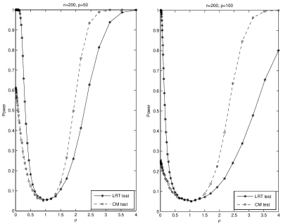
Figure 1: Empirical performances of LRT and CM tests for Gaussian data with known means.

For general data, due to the CM test is only applicable for $N_{p}(0,\Sigma_{p})$, we conduct comparisons between LRT and the test of Chen et al. (2010) (CZZ test) where $Y_{ij}$ comes from Gamma(4, 0.5) distribution in data (4). Figure 2 reports the empirical powers of the LRT and CZZ tests and the conclusions follow very similar patterns to those of Figure 1 which shows that LRT is a powerful test to detect eigenvalues around zero.

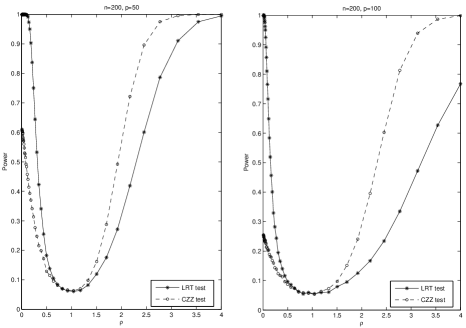
Figure 2: Empirical performances of LRT and CZZ tests for non-Gaussian data with unknown means

4 Appendix

4.1 Proof of Theorem 2

Writing

$$B_{n}=\frac{1}{n-1}\sum_{k=1}^{n}(Y_{k}-\bar{Y})(Y_{k}-\bar{Y})^{\prime},$$ (12)

where $\bar{Y}=\sum_{k=1}^{n}Y_{k}$. Noting $S_{n}=\Sigma_{p}^{1/2}B_{n}\Sigma_{p}^{1/2}$, we have

$$L_{n} = \frac{1}{p}\rm{tr}(S_{n})-\frac{1}{p}\log{|S_{n}|}-1-d(y_{n})$$

$$= \frac{1}{p}\rm{tr}(\Sigma_{p}B_{n})-\frac{1}{p}\rm{tr}(B_{n})-\frac{1}{p}\log{|\Sigma_{p}|}+BL_{n}$$

$$= BL_{n}+\frac{1}{p}L_{l}(\Sigma_{p})+\frac{1}{p}\rm{tr}((\Sigma_{p}-I_{p})B_{n})-\frac{1}{p}\rm{tr}(\Sigma_{p}-I_{p}),$$

where $BL_{n}=\frac{1}{p}\rm{tr}(B_{n})-\frac{1}{p}\log{|B_{n}|}-1-d(y_{n})$. By Theorem 1,

$$\frac{pBL_{n}-\mu_{n}}{\sigma_{n}}\stackrel{{\scriptstyle D}}{{\rightarrow}}N(0,1).$$

Therefore, to prove Theorem 2, it is enough to show

$$\epsilon_{n}:=\rm{tr}((\Sigma_{p}-I_{p})B_{n})-\rm{tr}(\Sigma_{p}-I_{p})=o_{p}(1).$$

Rewriting $B_{n}$ as

$$B_{n}=\frac{1}{n}\sum_{k=1}^{n}Y_{k}Y_{k}^{\prime}-\frac{1}{n(n-1)}\sum_{i\neq j}Y_{i}Y_{j}^{\prime},$$ (13)

we can get $E[\epsilon_{n}]=0$ and by Proposition A.1 of Chen et al. (2010),

$$E[\epsilon_{n}^{2}] = E[(\frac{1}{n}\sum_{k=1}^{n}Y_{k}^{\prime}(\Sigma_{p}-I_{p})Y_{k}-\frac{1}{n(n-1)}\sum_{i\neq j}Y_{i}^{\prime}(\Sigma_{p}-I_{p})Y_{j})^{2}]-(\rm{tr}(\Sigma_{p}-I_{p}))^{2}$$

$$= \frac{2}{n-1}\rm{tr}((\Sigma_{p}-I_{p})^{2})+\frac{\Delta}{n}tr((\Sigma_{p}-I_{p})\circ(\Sigma_{p}-I_{p}))$$

$$\leq \frac{2+\Delta}{n-1}\rm{tr}((\Sigma_{p}-I_{p})^{2})$$

where $\circ$ denotes Hadamard product. Above all, when $p/n\to y$ and $\rm{tr}((\Sigma_{p}-I_{p})^{2})/p\to 0$, we come to $\epsilon_{n}=o_{p}(1)$.

The proof is completed.

4.2 Proof of Theorem 3

To prove the theorem, we need some inequalities.

Lemma 1

For any $x>0$,

• If $0<x\leq 1$, $(x-1)^{2}\leq 2(x-1-\log{x})$;

• If $1<x<M$, $(x-1)^{2}\leq 2M(x-1-\log{x})$.

Since $L_{l}(\Sigma_{p})\to b\in(0,\infty)$, for large enough $p$, we will always have $D_{1}(\Sigma_{p})<2b$. Denoting the eigenvalues of $\Sigma_{p}$ as $\lambda_{1,p},\cdots,\lambda_{p,p}$,

$$L_{l}(\Sigma_{p})=\sum_{k=1}^{p}(\lambda_{k,p}-\log{\lambda_{k,p}}-1)<2b,$$

which implies that there is a constant $c_{0}=c_{0}(b)>1$ satisfying

$$c_{0}^{-1}\leq\lambda_{1,p},\cdots,\lambda_{p,p}\leq c_{0}.$$

By Lemma 1, $(\lambda_{k,p}-1)^{2}\leq 2c_{0}(\lambda_{k,p}-\log{\lambda_{k,p}}-1)$ which means

$$L_{q}(\Sigma_{p})=\sum_{k=1}^{p}(\lambda_{k,p}-1)^{2}\leq 2c_{0}L_{l}(\Sigma_{p})<4c_{0}b=o(p).$$

By Theorem 2 and Slutsky’s lemma,

$$\frac{pL_{n}-\mu_{n}}{\sigma_{n}}-\frac{b}{\sqrt{-2y-2\log{(1-y)}}}\stackrel{{\scriptstyle D}}{{\rightarrow}}N(0,1).$$

Now, we can calculate the power of the test

$$P_{\Sigma_{p}}(\phi~{}rejects~{}H_{0})=P(\frac{pL_{n}-\mu_{n}}{\sigma_{n}}>z_{1-\alpha})$$

$$= P(\frac{pL_{n}-\mu_{n}}{\sigma_{n}}-\frac{b}{\sqrt{-2y-2\log{(1-y)}}}>z_{1-\alpha}-\frac{b}{\sqrt{-2y-2\log{(1-y)}}})$$

$$\to 1-\Phi(z_{1-\alpha}-\frac{b}{\sqrt{-2y-2\log{(1-y)}}}).$$

The proof is completed.

References

• Anderson (2003) Anderson, T. (2003). An introduction to multivariate statistical analysis. Hoboken, NJ:Wiley.
• Bai etΒ al. (2009) Bai, Z., Jiang, D., Yao, J., and Zheng, S. (2009). Corrections to LRT on large-dimensional covariance matrix by rmt. The Annals of Statistics, 37(6B), 3822–3840.
• Birke and Dette (2005) Birke, M. and Dette, H. (2005). A note on testing the covariance matrix for large dimension. Statistics & Probability Letters, 74(3), 281–289.
• Cai and Jiang (2011) Cai, T. and Jiang, T. (2011). Limiting laws of coherence of random matrices with applications to testing covariance structure and construction of compressed sensing matrices. The Annals of Statistics, 39(3), 1496–1525.
• Cai and Ma (2012) Cai, T. and Ma, Z. (2012). Optimal hypothesis testing for high dimensional covariance matrices. arXiv:1205.4219.
• Chen etΒ al. (2010) Chen, S., Zhang, L., and Zhong, P. (2010). Tests for high-dimensional covariance matrices. Journal of the American Statistical Association, 105(490), 810–819.
• Dempster (1958) Dempster, A. (1958). A high dimensional two sample significance test. The Annals of Mathematical Statistics, 29(4), 995–1010.
• Jiang etΒ al. (2012) Jiang, D., Jiang, T., and Yang, F. (2012). Likelihood ratio tests for covariance matrices of high-dimensional normal distributions. Journal of Statistical Planning and Inference.
• Johnstone (2001) Johnstone, I. (2001). On the distribution of the largest eigenvalue in principal components analysis. The Annals of Statistics, 29(2), 295–327.
• Ledoit and Wolf (2002) Ledoit, O. and Wolf, M. (2002). Some hypothesis tests for the covariance matrix when the dimension is large compared to the sample size. The Annals of Statistics, pages 1081–1102.
• Li and Chen (2012) Li, J. and Chen, S. (2012). Two sample tests for high-dimensional covariance matrices. The Annals of Statistics, 40(2), 908–940.
• Nagao (1973) Nagao, H. (1973). On some test criteria for covariance matrix. The Annals of Statistics, pages 700–709.
• Onatski etΒ al. (2011) Onatski, A., Moreira, M., and Hallin, M. (2011). Asymptotic power of sphericity tests for high-dimensional data. Manuscript.
• Schott (2006) Schott, J. (2006). A high-dimensional test for the equality of the smallest eigenvalues of a covariance matrix. Journal of Multivariate Analysis, 97(4), 827–843.
• Srivastava (2005) Srivastava, M. (2005). Some tests concerning the covariance matrix in high dimensional data. J. Japan Statist. Soc, 35(2), 251–272.
• Wang etΒ al. (2012) Wang, C., Yang, J., Miao, B., and Cao, L. (2012). On identity tests for high dimensional data using rmt. arXiv:1203.3278.