Constraint-based reachability

Abstract

Iterative imperative programs can be considered as infinite-state systems computing over possibly unbounded domains. Studying reachability in these systems is challenging as it requires to deal with an infinite number of states with standard backward or forward exploration strategies. An approach that we call Constraint-based reachability, is proposed to address reachability problems by exploring program states using a constraint model of the whole program. The keypoint of the approach is to interpret imperative constructions such as conditionals, loops, array and memory manipulations with the fundamental notion of constraint over a computational domain. By combining constraint filtering and abstraction techniques, Constraint-based reachability is able to solve reachability problems which are usually outside the scope of backward or forward exploration strategies. This paper proposes an interpretation of classical filtering consistencies used in Constraint Programming as abstract domain computations, and shows how this approach can be used to produce a constraint solver that efficiently generates solutions for reachability problems that are unsolvable by other approaches.

1 Introduction

Modern automated program verification can be seen as the convergence of three distinct approaches, namely Software Testing, Model-Checking and Program Proving. Even if the general verification problems are often undecidable, investigations on these approaches have delivered the most efficient automated techniques to show that a given property is satisifed or not by all the reachable states of an infinite-state system.

Several authors have advocated the usage of constraints to represent an infinite set of states and the usage of constraint solvers to efficiently address reachability problems [7, 14, 17, 5]. In automated program verification problems, the goal is to find a state of the program which violates a given safety property, i.e., an unsafe state. Two distinct strategies have been investigated to explore programs with constraints, namely the forward analysis and the backward analysis strategies. In forward analysis, a set of reachable states is explored by computing the transition from the initial states of a program to the next states in forward way. If an unsafe state is detected to belong to the set of reachable states during this exploration then a property violation is reported. In backward analysis, states are computed from an hypotetical unsafe state in a backward way with the hope to discover that one of those is actually an initial state. One advantage of backward analysis over forward analysis is its usage of the targeted unsafe state to refine the state search space. However, both strategies are quite powerful and have been implemented into several software model checkers based on constraint solving [26, 17] and automated test case generators [30, 19, 18, 9, 4].

In this paper, we present an integrated constraint-based strategy that can benefit from the strengths of both forward and backward analysis. The keypoint of the approach, that we have called Constraint-Based Reachability (CBR), is to interpret imperative constructions such as conditionals, loops, array and memory manipulations with the fundamental notion of constraint over a computational domain. By combining constraint filtering and abstraction techniques, CBR is able to solve reachability problems which are usually outside the scope of backward or forward exploration strategies. A main difference is that CBR does not sequentially explore the execution paths of the program ; the exploration is driven by the constraint solver which picks-up the constraint to explore depending on the priorities that are attached to them. It is worth noticing that applying CBR to program exploration results in a semi-correct procedure only, meaning that there is no termination guarantee. CBR has been mainly applied in automatic test data generation for iterative programs [22, 23], programs that manipulate pointers towards named locations of the memory [24, 25], programs on dynamic data structures and anonymous locations [8], programs containing floating-point computations [6]. A major improvement of the approach was brought by the usage of Abstract Interpretation techniques to enrich the filtering capabilities of the constraints used to represent conditionals and loops [15, 16]. This approach permitted us to build efficient test data generator tools for a subset of C [20] and Java Bytecode [9].

The first contribution of this paper is the interpretation of classical filtering consistencies notions in terms of abstract domain computations. Constraint filtering is the main approach behind the processing of constraints in a finite domains constraint solver. We show in general the existence of tight links between classical filtering techniques and abstract domain computations that were not pointed out elsewhere. We also give the definition of a new consistency filtering inspired from the Polyhedral abstract domain, as consequence of these links.

The second contribution is the description of a special constraint handling any iterative construction. The constraint w captures iterative reasoning in a constraint solver and as such, is able to deduce information which is outside the scope of any pure forward or backward abstract analyzer. Its filtering capabilities combines both constraint reasoning and abstract domain computations in order to propagate informations to the rest of the constraint system. In this paper, we focus on the theoretical foundations of the constraints, while giving examples of its usage for test case generation over iterative programs.

Outline of the paper. The rest of the paper is organized as follows. Sec.2 introduces the necessary background in Abstract Interpretation to understand the contributions of the paper. Sec.3 establishes the link between classical constraint filtering and abstract domain computations. Sec.4 describes the theoretical foundation of the w constraint for handling iterative constructions while Sec.5 concludes the paper.

2 Background

Abstract Interpretation (AI) is a theoretical framework introduced by Cousot and Cousot in [11] to manipulate abstractions of program states. An abstraction can be used to simplify program analysis problems otherwise not computable in realistic time, to manageable problems more easily solvable. Instead of working on the concrete semantics of a program, AI computes results over an abstract semantics allowing so to produce over-approximating properties of the concrete semantics. In the following we introduce the basic notions required to understand AI.

Definition 1 (Partially ordered set (poset))

Let $\sqsubseteq$ be a partial order law, then the pair $(\mathcal{D},\sqsubseteq)$ is called a poset iff

$$\begin{array}[]{ll}\forall x\in\mathcal{D},x\sqsubseteq x&\textrm{{(reflexive)}}\\ \forall x,y\in\mathcal{D},x\sqsubseteq y\land y\sqsubseteq x\implies x=y&\textrm{{(anti-symmetry)}}\\ \forall x,y,z\in\mathcal{D},x\sqsubseteq y\land y\sqsubseteq z\implies x\sqsubseteq z&\textrm{{(transitive)}}\\ \end{array}$$

Definition 2 (Complete lattice)

A complete lattice is a 4-tuple $(\mathcal{D},\sqsubseteq,\bigsqcup,\bigsqcap)$ such that

• $(\mathcal{D},\sqsubseteq)$ is a poset

• $\bigsqcup$ is a upper bound: $\forall\mathcal{S}\subseteq\mathcal{D}$, we have

  $$\forall x\in\mathcal{S},x\sqsubseteq\bigsqcup\mathcal{S}$$

  $$\forall y\in\mathcal{D},(\forall x\in\mathcal{S},x\sqsubseteq y)\implies\bigsqcup\mathcal{S}\sqsubseteq y$$

• $\bigsqcap$ is a lower bound: $\forall\mathcal{S}\subseteq\mathcal{D}$, we have

  $$\forall x\in\mathcal{S},\bigsqcap\mathcal{S}\sqsubseteq x$$

  $$\forall y\in\mathcal{D},(\forall x\in\mathcal{S},y\sqsubseteq x)\implies y\sqsubseteq\bigsqcap\mathcal{S}$$

Complete lattices have a single smallest element $\bot=\bigsqcap\mathcal{D}$ and a single greatest element $\top=\bigsqcup\mathcal{D}$. Program semantics can usually be expressed as the least fix point of a monotonic and continuous function. A function $f$ from a complete lattice $(\mathcal{D},\sqsubseteq,\bigsqcup,\bigsqcap)$ to itself is monotonic iff $\forall l_{1},l_{2}\in\mathcal{D},l_{1}\sqsubseteq l_{2}\implies f(l_{1})\sqsubseteq f(l_{2})$. It is continuous iff $\forall\mathcal{S}\subseteq\mathcal{D},f(\bigsqcup\mathcal{S})=\bigsqcup_{s\in\mathcal{S}}(f(s))$ and $f(\bigsqcap\mathcal{S})=\bigsqcap_{s\in S}(f(s))$.

The following Theorem guarantees the existence of the fix points of a monotonic function.

Theorem 1 (Knaster-Tarski)

In a complete lattice $(\mathcal{D},\sqsubseteq,\bigsqcup,\bigsqcap)$, for all monotonic functions
$f:\mathcal{D}\rightarrow\mathcal{D}$,

• the least fix point of $f$ (i.e., $lfp(f)$) exists and $lfp(f)=\bigsqcap\{x\leavevmode\nobreak\ |\leavevmode\nobreak\ f(x)\sqsubseteq x\}$

• the greatest fix point of $f$ (i.e., $gfp(f)$) exists and $gfp(f)=\bigsqcup\{x\leavevmode\nobreak\ |\leavevmode\nobreak\ f(x)\sqsubseteq x\}$

In addition, when the functions are continuous, these fix points can be computed using an algorithm derived from the following theorem:

Theorem 2 (Kleene)

In a complete lattice $(\mathcal{D},\sqsubseteq,\bigsqcup,\bigsqcap)$, for all monotonic and continuous functions $f:\mathcal{D}\rightarrow\mathcal{D}$, the least fix point of $f$ is equal to $\bigsqcup\{f^{n}(\bot)\leavevmode\nobreak\ |\leavevmode\nobreak\ n\in\mathbb{N}\}$ and the greatest fix point of $f$ is equal to $\bigsqcap\{f^{n}(\top)\leavevmode\nobreak\ |\leavevmode\nobreak\ n\in\mathbb{N}\}$

As $\bot,f(\bot),\ldots,f^{n}(\bot),\ldots$ is an increasing suite, we get $\bigsqcup\{f^{n}(\bot)\leavevmode\nobreak\ |\leavevmode\nobreak\ n\leq k\}=f^{k}(\bot)$. Hence, $\textrm{lfp}(f)=\lim_{k\rightarrow+\infty}f^{k}(\bot)$ and $\textrm{gfp}(f)=\lim_{k\rightarrow+\infty}f^{k}(\top)$.

For reaching the least fix point of a monotonic and continuous function in a complete lattice, it suffices to iterate $f$ from $\bot$ until a fix point is reached.

Let $(\mathcal{D},\sqsubseteq,\bigsqcup,\bigsqcap)$ be a complete lattice called the concrete lattice and $f$ a function that defines some concrete semantics over this lattice, let $(\mathcal{D}^{\sharp},\sqsubseteq^{\sharp})$ be a poset called the abstract poset, and $f^{\sharp}:\mathcal{D}^{\sharp}\rightarrow\mathcal{D}^{\sharp}$ be a continuous function, then Abstract Interpretation aims at computing a fix point of $f^{\sharp}$ in order to over-approximate the computation performed by $f$.

Depending on whether the abstract poset is a complete lattice or not, we have distinct theoretical results regarding the abstraction. Proofs of the following theorems can be found in [12].

Galois connection

When the abstract poset is a complete lattice, the notion of Galois connection is available to link the abstract computations with the concrete lattice.

Definition 3 (Galois connection)

Let $(\mathcal{D},\sqsubseteq,\bigsqcup,\bigsqcap)$ and $(\mathcal{D}^{\sharp},\sqsubseteq^{\sharp},\bigsqcup^{\sharp},\bigsqcap^{\sharp})$ be two complete lattices, then a pair of functions $\alpha:\mathcal{D}\rightarrow\mathcal{D}^{\sharp}$ and $\gamma:\mathcal{D}^{\sharp}\rightarrow\mathcal{D}$ is a Galois connection iff $\forall x\in\mathcal{D},\forall y\in\mathcal{D}^{\sharp},\alpha(x)\sqsubseteq^{\sharp}y\iff x\sqsubseteq\gamma(y)$ noted:

$(\mathcal{D},\sqsubseteq,\bigsqcup,\bigsqcap)\overset{\gamma}{\underset{\alpha}{\leftrightarrows}}(\mathcal{D}^{\sharp},\sqsubseteq^{\sharp},\bigsqcup^{\sharp},\bigsqcap^{\sharp})$

Next definition establishes the correction property of an analysis.

Definition 4 (Sound approximation)

Let $(\mathcal{D},\sqsubseteq,\bigsqcup,\bigsqcap)\overset{\gamma}{\underset{\alpha}{\leftrightarrows}}(\mathcal{D}^{\sharp},\sqsubseteq^{\sharp},\bigsqcup^{\sharp},\bigsqcap^{\sharp})$ be a Galois connection, then a function $f^{\sharp}:\mathcal{D}^{\sharp}\rightarrow\mathcal{D}^{\sharp}$ is a sound approximation of $f:\mathcal{D}\rightarrow\mathcal{D}$ iff

$$\forall y\in\mathcal{D}^{\sharp},f\circ\gamma(y)\sqsubseteq\gamma\circ f^{\sharp}(y)$$

Consquently, we have the following notion:

Theorem 3 (Smallest sound approximation)

Let $(\mathcal{D},\sqsubseteq,\bigsqcup,\bigsqcap)\overset{\gamma}{\underset{\alpha}{\leftrightarrows}}(\mathcal{D}^{\sharp},\sqsubseteq^{\sharp},\bigsqcup^{\sharp},\bigsqcap^{\sharp})$ be a Galois connection, and a function $f:\mathcal{D}\rightarrow\mathcal{D}$, then the smallest sound approximation of $f$ is $\alpha\circ f\circ\gamma$

This theorem implies that any function greater than $\alpha\circ f\circ\gamma$ is a sound approximation of $f$ and the following theorem characterizes the results of fixpoint computations:

Theorem 4 (Fixpoint computations with sound approximation)

Let $(\mathcal{D},\sqsubseteq,\bigsqcup,\bigsqcap)\overset{\gamma}{\underset{\alpha}{\leftrightarrows}}(\mathcal{D}^{\sharp},\sqsubseteq^{\sharp},\bigsqcup^{\sharp},\bigsqcap^{\sharp})$ be a Galois connection, let $f^{\sharp}:\mathcal{D}^{\sharp}\rightarrow\mathcal{D}^{\sharp}$ and $f:\mathcal{D}\rightarrow\mathcal{D}$ be two monotonic functions such that $f^{\sharp}$ is a sound approximation of $f$, then, we have:

$$\textrm{lfp}(f)\sqsubseteq\gamma(\textrm{lfp}(f^{\sharp}))\leavevmode\nobreak\ \textrm{and}$$

$$\textrm{gfp}(f)\sqsubseteq\gamma(\textrm{gfp}(f^{\sharp}))$$

Intuitively, this theorem gives a process to compute an over-approximation by Abstract Interpretation, as shown in Fig 1.

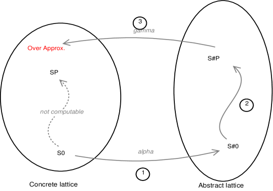
Figure 1: Static approximations of fixed point computations in complete lattices

The left part shows the concrete lattice where the concrete computation of $f$ is performed starting from initial state $S_{0}$. The right part shows the abstract lattice that is used to over-approximate the computation. This computation is undertaken in three steps:

• initial state abstraction;

• fixpoint computation in the abstract lattice;

• result concretization.

Without Galois connection

When the abstract lattice is not complete, there does not exist necessarily a best abstraction for all elements of the concrete lattice. The notion of Galois connection is no more available and the abstract lattice is just linked with the concrete lattice through a monotonic function $\gamma:\mathcal{D}^{\sharp}\rightarrow\mathcal{D}$. The definition of sound approximation needs to be adapted:

Definition 5 (Sound approximation without a Galois connection)

Let $(\mathcal{D},\sqsubseteq)$ and $(\mathcal{D}^{\sharp},\sqsubseteq^{\sharp})$ be two posets, let $\gamma:\mathcal{D}^{\sharp}\rightarrow\mathcal{D}$ be a monotonic function and $f:\mathcal{D}\rightarrow\mathcal{D}$ a function, then the function $f^{\sharp}:\mathcal{D}^{\sharp}\rightarrow\mathcal{D}^{\sharp}$ is a sound approximation of $f$ iff

$$\forall x\in\mathcal{D}^{\sharp},f\circ\gamma(x)\sqsubseteq\gamma\circ f^{\sharp}(x)$$

In such an (not complete) abstract lattice, nothing guarantees the existence of the least fix point: $\textrm{lfp}(f)$ is not necessarily approximated by $\textrm{lfp}(f^{\sharp})$. However, any fix point of $f^{\sharp}$ can be used:

Theorem 5

Let $(\mathcal{D},\sqsubseteq,\bigsqcup,\bigsqcap)$ be a complete lattice, and $(\mathcal{D}^{\sharp},\sqsubseteq^{\sharp})$ be a poset, let $\gamma:\mathcal{D}^{\sharp}\rightarrow\mathcal{D}$, $f:\mathcal{D}\rightarrow\mathcal{D}$ and $f^{\sharp}:\mathcal{D}^{\sharp}\rightarrow\mathcal{D}^{\sharp}$ be three monotonic functions then if $f^{\sharp}$ is a sound approximation of $f$, then we have:

$$\forall x\in\mathcal{D}^{\sharp},f^{\sharp}(x)=x\implies\textrm{lfp}(f)\sqsubseteq\gamma(x)$$

Next theorem is useful to compute an over-approximation of $\textrm{gfp}(f)$ when the lattice is not complete:

Theorem 6

Let $(\mathcal{D},\sqsubseteq,\bigsqcup,\bigsqcap)$ be a complete lattice, let $(\mathcal{D}^{\sharp},\sqsubseteq^{\sharp})$ be a poset with a greatest element $\top$ and let $\gamma:\mathcal{D}^{\sharp}\rightarrow\mathcal{D}$, $f:\mathcal{D}\rightarrow\mathcal{D}$ and $f^{\sharp}:\mathcal{D}^{\sharp}\rightarrow\mathcal{D}^{\sharp}$ be three monotonic functions, then
if $f^{\sharp}$ is a sound approximation of $f$ and $a$ is an element of $\mathcal{D}^{\sharp}$ such that there exists $k$ such as $a={f^{\sharp}}^{k}(\top)$, then

$$\textrm{gfp}(f)\sqsubseteq\gamma(a)$$

Consequently, when the abstract lattice is not complete, instead of abstracting the initial state, one selects an element of the abstract lattice that over-approximates the initial state. And, a fix point is computed in the abstract lattice from this element. The fix point is still an over-approximation of the concrete semantics.

2.1 Examples of abstract domains

In this section, we briefly describe two abstract domains: the Interval [13] and the Polyhedral [12] domains.

2.1.1 The Interval abstract domain

Interval analysis aims at approximating a set of values by an interval of possible values. If $\mathcal{I}_{\mathbb{N}}=\{[a,b]\leavevmode\nobreak\ |\leavevmode\nobreak\ a,b\in\mathbb{N}\cup\{-\infty,+\infty\}\}$, then the Interval abstract domain is the Cartesian product $\mathcal{I}_{\mathbb{N}}\times...\times\mathcal{I}_{\mathbb{N}}$ equipped with inclusion, union and intersection over intervals. This abstract domain is a complete lattice.

State abstraction is performed by computing an interval that over-approximates the set of possible values for each variable. If the concrete state is an unbounded set of tuples $\{(x_{11},\ldots,x_{n1}),(x_{12},\ldots,x_{n2}),\ldots\}$ then:

$$\alpha(\{(x_{11},\ldots,x_{n1}),(x_{12},\ldots,x_{n2}),\ldots\})=([m_{1},M_{1}],\ldots,[m_{n},M_{n}])\\ \leavevmode\nobreak\ \textrm{with}\leavevmode\nobreak\ m_{i}=\left\{\begin{array}[]{ll}min_{j}(x_{ij})\leavevmode\nobreak\ \textrm{if it exists}\\ -\infty\leavevmode\nobreak\ \textrm{else}\end{array}\right.\leavevmode\nobreak\ \textrm{and}\leavevmode\nobreak\ M_{i}=\left\{\begin{array}[]{ll}max_{j}(x_{ij})\leavevmode\nobreak\ \textrm{if it exists}\\ +\infty\leavevmode\nobreak\ \textrm{else}\end{array}\right.$$

The concretization of an abstract state is obtained by computing the Cartesian product of the intervals. These functions define a Galois connection between the concrete domain and the abstract domain of intervals.

The approximation of transfert functions is realized by using their structure and classical results from Interval Analysis [28]. For example, functions $[x\leq y]$ and $[x=y+z]$ are abstracted by the following (sound) approximations: $[x\leq y]^{\sharp}:([a,b],[c,d])\rightarrow([a,min(b,d)],[max(a,c),d]))$ and $[x=y+z]^{\sharp}:([a,b],[c,d],[e,f])\rightarrow([c+e,d+f]\cap^{\sharp}[a,b],[a-f,e-b]\cap^{\sharp}[c,d],[a-d,c-b]\cap^{\sharp}[e,f])$.

2.1.2 The Polyhedral abstract domain

In Polyhedral analyses, each concrete state is abstracted by a conjunction of linear constraints that defines a convex polyhedron. Indeed, a convex polyhedron is a region of an n-dimensional space that is bounded by a finite set of hyperplanes ${x\in IR^{n}|ax\geq c}$ where $a\in IR^{n}$ and $c\in IR$. The abstract lattice equiped with inclusion, convex hull, and intersection of polyhedra is not a complete lattice as there is no upper bound to the convex union of all the convex polyhedra that can be written in a circle.

Abstract functions can be defined to deal with polyhedra. For example:

$$[x\geq y]^{\sharp}(\{z\leq x+y\}) = \{z\leq x+y,y\leq x\}$$ (1)

$$[x>y]^{\sharp}(\{x\leq y\}) = \{0=1\}$$ (2)

$$[x=y*z]^{\sharp}(\{1\leq y\leq 10\}) = \{x\leq z,x\leq 10*z\}$$ (3)

If the expression is a linear condition, then it is just added to the polyhedron (case 1). If the expression is contradictory with the current polyhedron, then it is reduced to $1=0$ meaning that there is no abstract (and concrete) state in the approximation (case 2). If the expression is non-linear, then a linear approximation is derived when available and added to the polyhedron (case 3).

3 Filtering consistencies as abstract domain computations

As noticed by Apt [2], constraint propagation algorithms can be seen as instances of algorithms that deal with chaotic iteration. In this context, chaotic means fair application of propagators until saturation. In this section, we elaborate on a bridge between two unrelated notions: filtering consistencies and abstract domains. In particular, we show that arc– and bound– consistency are instances of chaotic iterations over two distinct abstract domains. Classical AI notions of sound approximation and abstract domain computations, not used in [2], allows to show that filtering consistencies compute sound over-approximations of the solutions set of a constraint system. Thanks to the bridge, we also propose new filtering consistency algorithms based on the polyhedral abstract domain.

3.1 Notations

Let $ZZ$ be the set of integers and $\cal V$ be a finite set of integer variables, where each variable $x$ in $\cal V$ is associated with a finite domain $D(x)$. The domain $\mathcal{D}$ is the Cartesian product of each variable domain: $D(x_{1})\times\ldots\times D(x_{m})$ and $\mathcal{P(D)}$ denotes the powerset of $\mathcal{D}$. $inf_{\mathcal{D}}x$ and $sup_{\mathcal{D}}x$ denote respectivelly the inferior and the superior bounds of $D(x)$ in $\mathcal{D}$. A constraint $c$ is a relation between variables of $\cal V$. The language of (elementary) constraints is built over arithmetical operators $\{+,-,*,\,...\}$ and relational operators $\{<,\leq,>,\geq,=,\neq,...\}$ but any relation over a subset of $\cal V$ can be considered. Let vars$(c)$ be the function that returns the variables of $\cal V$ appearing in a constraint $c$. A valuation $\sigma$ is a mapping of variables to values, noted $\{x_{1}\mapsto d_{1},...,x_{n}\mapsto d_{n}\}$. $CS$ denotes a constraint system $CS$, i.e., a finite set of constraints.

3.2 Exact filtering

Let $\{c_{1},..,c_{m}\}$ be a $CS$ over $\{x_{1},..,x_{n}\}$ and let $\mathcal{D}=D(x_{1})\times..\times D(x_{n})$, then the solution-set of $CS$ is an element of $\mathcal{P(D)}$, noted $sol(CS)$.

The exact filtering operator of a constraint $c_{i}$ is computed with the function $f_{i}:\mathcal{P}(\mathcal{D})\rightarrow\mathcal{P}(\mathcal{D})$ which maps an element $S\in\mathcal{P}(\mathcal{D})$ to $f_{i}(S)=\{s\leavevmode\nobreak\ |\leavevmode\nobreak\ s\in S\land c_{i}(s)\}$. The exact filtering operator of $c_{i}$ removes all the tuples of $\mathcal{D}$ that violate $c_{i}$. Hence, by using an iterating procedure, it permits to compute $sol(CS)$: if $f_{C}=f_{1}\circ\ldots\circ f_{m}$ then $sol(C)=\textrm{gfp}(f_{C})$. By noticing that $f_{C}$ is continuous (as each $f_{i}$ is continuous) and monotonic and thanks to Theorem 2 we get $sol(CS)=\lim_{k\rightarrow+\infty}{f_{C}}^{k}(\mathcal{D})$.

Example 1

Consider $CS=\{x\neq y,y\neq z,z\neq x\}$ where $x\in 1..2,y\in 1..2,z\in 1..2$. The exact filtering operator associated with $x\neq y$ will remove the tuples $(1,1,1),(1,1,2),(2,2,1),(2,2,2)$ from $\{1,2\}\times\{1,2\}\times\{1,2\}$. Iterating over all the constraints of $CS$ will eventually exhibit the inconsistency of this example.

In fact, this shows that exact filtering of a CS over $D(x_{1})\times..\times D(x_{n})$ can be reached if one computes over a complete lattice built over the set of possible valuations: $(\mathcal{P}(D(x_{1})\times..\times D(x_{n})),\subseteq,\bigcup,\bigcap)$. This lattice will be called the concrete lattice in the rest of the paper. Of course, computing over the concrete lattice is usually unreasonable, as it requires to examine every tuple of the Cartesian product $D(x_{1})\times..\times D(x_{n})$ w.r.t. consistency of each constraint.

3.3 Domain-consistency filtering

For binary constraint systems, the most successful local consistency filtering is arc-consistency, which ensures that every value in the domain of one variable has a support in the domain of the other variable. The standard extension of arc-consistency for constraints of more than two variables is domain-consistency (also called hyper-arc consistency [27]). Roughly speaking, the abstraction that underpins domain-consistency filtering aims at considering each variable domain separately, instead of considering the Cartesian product of each individual domain. More formally,

Definition 6 (Domain-consistency)

A domain $\mathcal{D}$ is domain-consistent for a constraint $c$ where $vars(c)=\{x_{1},..,x_{n}\}$ iff for each variable $x_{i}$, $1\leq i\leq n$ and for each $d_{i}\in D(x_{i})$ there exist integers $d_{j}$ with $d_{j}\in D(x_{j})$, $1\leq j\leq n,j\neq i$ such that $\sigma=\{x_{1}\mapsto d_{1},..,x_{n}\mapsto d_{n}\}$ is an integer solution of $c$.

Consider the domains $\mathcal{D}=D(x_{1})\times..\times D(x_{n})$ and $\mathcal{D}^{\sharp}_{arc}=\mathcal{P}(D(x_{1}))\times\ldots\times\mathcal{P}(D(x_{n}))$ and the abstraction function $\alpha_{arc}:\mathcal{P}(\mathcal{D})\rightarrow\mathcal{D}^{\sharp}_{arc}$ which maps $S\in\mathcal{P}(\mathcal{D})$ to

$$\alpha_{arc}(S)=(\{x_{1}\leavevmode\nobreak\ |\leavevmode\nobreak\ x\in S\},\ldots,\{x_{n}\leavevmode\nobreak\ |\leavevmode\nobreak\ x\in S\})$$

The concretization function is a function $\gamma_{arc}:\mathcal{D}^{\sharp}_{arc}\rightarrow\mathcal{P}(\mathcal{D})$ such that

$$\gamma_{arc}((S_{1},\ldots,S_{n}))=S_{1}\times\ldots\times S_{n}$$

If $\sqsubseteq^{\sharp}_{arc}$, $\bigsqcup^{\sharp}_{arc}$ and $\bigsqcap^{\sharp}_{arc}$ denote respectivelly the inclusion, union and intersection of two tuples of sets, then we got the following Galois connection:

$(\mathcal{P}(\mathcal{D}),\subseteq,\bigcup,\bigcap)\overset{\gamma_{arc}}{\underset{\alpha_{arc}}{\leftrightarrows}}(\mathcal{D}^{\sharp}_{arc},\sqsubseteq^{\sharp}_{arc},\bigsqcup^{\sharp}_{arc},\bigsqcap^{\sharp}_{arc})$

The proof follows comes the monotonicity of the projection and Cartesian product. From Theorem 3, we get:

Definition 7

The best sound approximation of the exact filtering operator $f_{i}$ is

$$f_{i\_arc}^{\sharp}\overset{\operatorname{def}}{=}\alpha_{arc}\circ f_{i}\circ\gamma_{arc}$$

Theorem 7

Let $p$ be a filtering operator associated with constraint $c_{i}$, then $p$ computes domain-consistency iff $p=f_{i\_arc}^{\sharp}$.

This theorem implies that domain-consistency is the strongest property that can be guaranteed by a filtering operator using the abstraction $\alpha_{arc}$. A proof is given in the Appendix of the paper.

Let us consider now the function $f^{\sharp}_{arc}$ such that $f^{\sharp}_{arc}=f_{1\_arc}^{\sharp}\circ\ldots\circ f_{n\_arc}^{\sharp}$. As $f^{\sharp}_{arc}$ is a sound approximation of $f_{C}$ then

$$sol(C)=\textrm{gfp}(f_{C})\subseteq\gamma_{arc}(\textrm{gfp}(f^{\sharp}_{arc}))$$

This result shows if necessary that constraint propagation over domain-consistency filtering operators computes an over-approximation of the solution set of $C$.

3.4 Bound-consistency filtering

Following the same scheme, AI can be used to show the abstraction that underpins constraint propagation with bound-consistency filtering (also called interval-consistency). But, firstly, let us recall the definition of bound-consistency we consider in this paper, as several definitions exist in the literature [10] :

Definition 8 (Bound-consistency)

A domain $\mathcal{D}$ is bound-consistent for a constraint $c$ where $vars(c)=\{x_{1},..,x_{n}\}$ iff for each variable $x_{i}$, $1\leq i\leq n$ and for each $d_{i}\in\{inf_{\mathcal{D}}x_{i},sup_{\mathcal{D}}x_{i}\}$ there exist integers $d_{j}$ with $inf_{\mathcal{D}}x_{j}\leq d_{j}\leq sup_{\mathcal{D}}x_{j}$, $1\leq j\leq n,j\neq i$ such that $\sigma=\{x_{1}\mapsto d_{1},..,x_{n}\mapsto d_{n}\}$ is an integer solution of $c$.

Roughly speaking, this approximation considers only the bounds of the domain of each variable and approximates each domain with an interval. Let $\mathcal{I}(S)=[min(S),max(S)]$ be the smallest interval that contains all the elements of a finite set of integers $S$. Similarly, $\mathcal{I}^{-1}(I)$ denotes the set of integers of an interval $I$ : $\mathcal{I}^{-1}([a,b])=\{x\in\mathbb{Z}\leavevmode\nobreak\ |\leavevmode\nobreak\ a\leq x\leq b\}$.

The abstract domain we consider for bound-consistency is $\mathcal{D}^{\sharp}_{bound}=\mathcal{I}(\mathcal{P}(D(x_{1})))\times\ldots\times\mathcal{I}(\mathcal{P}(D(x_{n})))$.

Given a tuple of sets $(S_{1},\ldots,S_{n})$ and a tuple of intervals $(I_{1},\ldots,I_{n})$, we consider the functions $\alpha_{inter}$ and $\gamma_{inter}$ such that:

$$\alpha_{inter}(S_{1},\ldots,S_{n})=(\mathcal{I}(S_{1}),\ldots,\mathcal{I}(S_{n}))$$

$$\gamma_{inter}(I_{1},\ldots I_{n})=(\mathcal{I}^{-1}(I_{1}),\ldots,\mathcal{I}^{-1}(I_{n}))$$

Let $\alpha_{bound}:\mathcal{P}(\mathcal{D})\rightarrow\mathcal{D}^{\sharp}_{bound}$ be an abstraction function such that

$$\alpha_{bound}=\alpha_{inter}\circ\alpha_{arc}$$

and $\gamma_{bound}:\mathcal{D}^{\sharp}_{bound}\rightarrow\mathcal{P}(\mathcal{D})$ be a concretization function such that

$$\gamma_{bound}=\gamma_{arc}\circ\gamma_{inter}$$

If $\sqsubseteq^{\sharp}_{bound}$, $\bigsqcup^{\sharp}_{bound}$ and $\bigsqcap^{\sharp}_{bound}$ respectively denote inclusion, union and intersection of intervals (component by component) then we get the following Galois connection:

$(\mathcal{P}(\mathcal{D}),\subseteq,\bigcup,\bigcap)\overset{\gamma_{bound}}{\underset{\alpha_{bound}}{\leftrightarrows}}(\mathcal{D}^{\sharp}_{bound},\sqsubseteq^{\sharp}_{bound},\bigsqcup^{\sharp}_{bound},\bigsqcap^{\sharp}_{bound})$

Let $f_{i\_bound}^{\sharp}$ be the most accurate sound approximation of $f_{i}$, then we get:

$$f_{i\_bound}^{\sharp} = \alpha_{bound}\circ f_{i}\circ\gamma_{bound}$$

$$= \alpha_{inter}\circ f_{i\_arc}^{\sharp}\circ\gamma_{inter}$$

Theorem 8

If $p$ is a filtering operator associated to constraint $c_{i}$, then $p$ computes bound-consistency iff $p=f_{i\_bound}^{\sharp}$.

This theorem, proved in Appendix, implies that bound-consistency is the strongest property that can be reached with an operator based on the $\alpha_{bound}$ abstraction.

Consider now the function $f^{\sharp}_{bound}$ such that $f^{\sharp}_{bound}=f_{1\_bound}^{\sharp}\circ\ldots\circ f_{n\_bound}^{\sharp}$. As $f^{\sharp}_{bound}$ is a sound approximation of $f_{C}$, then

$$sol(C)=\textrm{gfp}(f_{C})\subseteq\gamma_{bound}(\textrm{gfp}(f^{\sharp}_{bound}))$$

This result shows if necessary that constraint propagation based on bound-consistency computes a sound over-approximation of the solution set of $C$. In addition, as $f^{\sharp}_{bound}$ is also a sound over-approximation of $f^{\sharp}_{arc}$, then

$$\gamma_{arc}(\textrm{gfp}(f^{\sharp}_{arc}))\subseteq\gamma_{bound}(\textrm{gfp}(f^{\sharp}_{bound}))$$

meaning that filtering with bound-consistency provides an over-approximation of the results given by a filtering with domain-consistency.

3.5 New filtering consistencies based on abstract domains

In the previous section, classical filtering consistencies are interpreted in terms of abstract domain computations. In this section, we propose a new filtering consistency based on the Polyhedral abstract domain [12].

3.5.1 Linear relaxations

When non-linear constraints are involved in a constraint store, approximating them with linear constraints is natural in order to benefit from powerful Linear Programming techniques. These techniques can be used to check the satisfiability of the constraint store when the approximation is sound. If the approximate constraint system is unsatisfiable so is the non-linear constraint system. But, in the context of optimization problems, the approximation can also be used to prune current bounds of the function to optimize.

Another form of approximation comes from the domain in which the computation occurs. A linear problem over integers can be relaxed in the domain of rationals or reals and solved within this domain. As the set of integers belongs to the rationals and reals, an integer solution of the relaxed problem is also a solution of the original integer problem, but the converse is false. In this paper, we will consider both kinds of approximations under the generic term of “linear relaxations”.

Computing a linear relaxation of a constraint system $CS$ aims at finding a set of linear constraints that characterizes an over-approximation of the solution set of $CS$. It is not unique but for trivial reasons, we are more interested in the tighter possible relaxations. The tightest linear relaxation is the convex hull of the solution set of $CS$ but computing this relaxation is as hard as solving $CS$. For $CS$ over finite domains, the problem is therefore NP_hard. Whenever a relaxation is computed by using the current bounds of variable domains, it is called dynamic and the consistencies presented in the rest of the section are compatible with dynamic linear relaxations.

3.5.2 Polyhedral-consistency filtering

Let $Poly$ be the abstract domain of closed convex polyhedra with rational coefficients. As said previously, $Poly$ is not a complete lattice, and then we cannot define a Galois connection between $Poly$ and the lattice of the solutions. Nevertheless, the concretization function $\gamma_{poly}:Poly\rightarrow\mathcal{P}(\mathcal{D})$ can be defined as the function that returns the integer points of a given polyhedron:

$$\gamma_{poly}(S^{\sharp})=\textrm{int\_sol}(S^{\sharp})$$

Here, int_sol stands for the whole set of integer solutions of a set of linear constraints As $S^{\sharp}$ is bounded, $\gamma_{poly}(S^{\sharp})$ is finite.

Without a Galois connection, we do not expect the polyhedral-consistency proposed in this section to be optimal w.r.t. the abstract domain. Hence, we only show that the filtering algorithm that computes this consistency is a sound approximation of the exact filtering operator.

Definition 9

Let $\alpha_{box}$ be the following abstraction function
$\alpha_{box}:\mathcal{D}_{bound}^{\sharp}\rightarrow Poly$ such that

$$\alpha_{box}(([a_{1},b_{1}],\ldots,[a_{m},b_{m}]))=\{a_{1}\leq x_{1}\leq b_{1},\ldots,a_{m}\leq x_{m}\leq bm\}$$

and the concretization function $\gamma_{box}:Poly\rightarrow\mathcal{D}_{bound}^{\sharp}$:

$$\gamma_{box}(P)=\left\{\begin{array}[]{l}([\lceil min(x_{1},P)\rceil,\lfloor max(x_{1},P)\rfloor],\ldots,[\lceil min(x_{m},P)\rceil,\lfloor max(x_{m},P)\rfloor])\\ \textrm{\leavevmode\nobreak\ \leavevmode\nobreak\ \leavevmode\nobreak\ \leavevmode\nobreak\ \leavevmode\nobreak\ \leavevmode\nobreak\ if\leavevmode\nobreak\ }\forall i,\lceil min(x_{i},P)\rceil\leq\lfloor max(x_{i},P)\rfloor\\ \emptyset\textrm{ otherwise}\end{array}\right.$$

where $\lfloor x\rfloor$ (resp. $\lceil x\rceil$) stands for the next smallest (resp. largest) integer of $x$, and $min(v,P)$ ( resp. $max(v,P)$) computes the smallest (resp. largest) value of $v$ corresponding to a point of $P$.

Both $\alpha_{box}$ and $\gamma_{box}$ link the polyhedral abstract domain with the interval abstract domain. The abstraction function $\alpha_{box}$ maps a set of intervals into a polyhedron by adding two inequalities per variable, while the concretization function $\gamma_{box}$ maps a polyhedron into a set of intervals by computing first the smallest hypercuboid containing the polyhedron and second the greatest hypercuboid with integer bounds. The behaviour of these two functions is illustrated in Fig. 2.

\psfrag{alphabox}{$\alpha_{box}$}\psfrag{gammabox}{$\gamma_{box}$}\includegraphics[width=312.9803pt,height=142.26378pt]{galois_box2.eps}

Figure 2: Connection between the Polyhedral and Interval abstract domains

Definition 10 (Polyhedral-consistency)

A domain $\mathcal{D}$ is polyhedral-consistent for a constraint $c$ where $vars(c)=\{x_{1},..,x_{n}\}$ iff for each variable $x_{i}$, $1\leq i\leq n$ and for each $d_{i}\in\{inf_{\mathcal{D}}x_{i},sup_{\mathcal{D}}x_{i}\}$ there exist rationals $r_{j}$ with $inf_{\mathcal{D}}x_{j}\leq r_{j}\leq sup_{\mathcal{D}}x_{j}$, $1\leq j\leq n,j\neq i$ such that $\sigma=\{x_{1}\mapsto r_{1},..,x_{n}\mapsto r_{n}\}$ is a (rational) solution of a linear relaxation of $c$.

The rationale behind this definition is to benefit from efficient polyhedral techniques over the rationals to filter the variation domain of variables. Of course, interesting implementations of this filtering consistency should trade between efficiency and precision as integer linear constraint solving is costly (NP_hard problem) even for bounded domains. It is worth noticing that the definition depends on the quality of the underlying linear relaxation. On the one hand, a linear relaxation which over-approximate $c$ by $True$ (the whole search space) is useless while on the other hand a linear relaxation which exploits piecewise over-approximations of $c$ is often too costly. We give examples of polyhedral-consistency filtering in function of various linear relaxations.

Example 2

Consider the following $CS$: $z=x+y,z=x*y$, let $c$ be the second constraint of $CS$: $c=(z=x*y)$ and let $\mathcal{D}$ be $x\in-7..10,y\in-7..10,z\in 3..10$.

Note that $\mathcal{D}$ is bound-consistent for all the constraints of $CS$.

The simplest linear relaxation that can be considered is the one that ignores non-linear constraints. In this example, $c$ is over-approximated by $True$ and then $\mathcal{D}$ viewed as $x\geq-7,x\leq 10,y\geq-7,x\leq 10,z\geq 3,x\leq 10,z=x+y$ is then polyhedral-consistant w.r.t. this linear relaxation. Note that this approach can be generalized by associating a new fresh variable to the non-linear term $x*y$ with a domain computed using the bounds $x$ and $y$. In this example, this does not help but it could help on other examples.

Another linear relaxation consists in building a polyhedron from the “bounds” of $x*y$ in $\mathcal{D}=x\in-7..10,y\in-7..10,z\in 3..10$. By considering the 2-dimensional polyhedron
$\{(1,10),(10,1),(-1,-7),(-7,-1)\}$ we get that a linear relaxation of $c$ in domain $\mathcal{D}$ is
$11x-8y+69\geq 0$
$-x-y+11\geq 0$
$-8x+11y+69\geq 0$
$x+y+8\geq 0$
Filtering with the polyhedral-consistency, we get that $x\in-2..9,y\in-2..9,z\in 3..10$ where $D(x)$ and $D(y)$ have been pruned. These results can be easily computed using a Linear Programming tool and truncation operators. For example, using the clpq library of SICStus Prolog which implements a simplex over the rationals, the following request permits to compute the max bound of variable $x$:

{X >= -7, X =< 10, Y >= -7, Y =< 10, Z >= 3, Z =< 10, Z = X+Y,
11*X - 8*Y+ 69 >=0, -X - Y + 11 >= 0, -8*X + 11*Y +69 >= 0,
X + Y + 8 >=0}, sup(X, R).

R = 179/19   % then max bound of x is 9

Finally, we can automate the computation of linear relaxations of $c$ by considering the following trivial constraints, which are always true for any $x$ and $y$: $(x-inf_{\mathcal{D}}x)(y-inf_{\mathcal{D}}y)\geq 0$
$(x-sup_{\mathcal{D}}x)(y-inf_{\mathcal{D}}y)\leq 0$
$(x-inf_{\mathcal{D}}x)(y-sup_{\mathcal{D}}y)\leq 0$
$(x-sup_{\mathcal{D}}x)(y-sup_{\mathcal{D}}y)\geq 0$

By decomposing these constraints, using the original bounds of $x,y,z$ and replacing the quadratic term $x*y$ by $z$, we get:
$7x+7y+z+49\geq 0$
$10x-7y-z+70\geq 0$
$-7x+10y-z+70\geq 0$
$-10x-10y+z+100\geq 0$
Filtering with the polyhedral-consistency, we get that $x\in-2..9,y\in-2..9,z\in 3..10$ where $D(x)$ and $D(y)$ have been pruned. These domains are still bound-consistent but another tighter relaxation can be computed with these new bounds:
$2X+2Y+Z+4=0$
$9X-2Y-Z+18=0$
$-2X+9Y-Z+18=0$
$-9X-9Y+Z+81=0$
and then filtering again permits to get that $x\in 0..8,y\in 0..8,z\in 3..10$. Here, filtering by bound-consistency leads to prune the domains to: $x\in 1..8,y\in 1..8,z\in 3..10$. Then, by iterating these two process, we get the only solution to $CS$ which is: $x\in 2..2,y\in 2..2,z\in 4..4$. This showed how dynamic linear relaxations can be used to solve a non-linear $CS$.

4 The w constraint operator

In this section, we present the w constraint operator which captures iterative computations, and how it is processed by a constraint solver. The constraint operator has been introduced a long time ago in [22, 23] and was further refined using Abstract Interpretation (AI) techniques [15]. In the following, we recall its interface and semantics and show how fixed point computations can be used to filter inconsistant values of the underlying relation. We also explain how the Polyhedral abstract domain is used to approximate the fixed point computations.

4.1 w as a relation over memory states

The $w$ operator captures a relation over three memory states that represent the state before, within and after the execution of an iterating statement. In this paper, we do not specify what a memory state is, or what the iterating statement is, as the approach is generic regarding the content of a memory state and the concrete syntax of the iterator. However, in order to ease the understanding, the reader can consider a memory state to be a mapping between variables of the program to values. More complex examples of memory states in relation with $w$ can be found in [8] and [9].

The relation w is expressed with the following syntax: $w(\mathcal{M}_{1},\mathcal{M}_{2},\mathcal{M}_{3},Dec,Body)\}$ where $\mathcal{M}_{1}$ denotes the memory state before execution of the iteration, $\mathcal{M}_{2}$ denotes the memory state reached at the end of execution of the $Body$, while $\mathcal{M}_{3}$ denotes the state after execution, $Dec$ is a boolean syntactical expression, and $Body$ is a list of statements. This three-states consideration is inspired by the Static Single Assignment of a program [29]. If the state of $\mathcal{M}$ is irrelevant for a given computation, we simply write $\_$. Note that $Body$ may also contain other iterators, and thus $w$ is meant to be a compositional operator. The semantics of $w$ is the semantics of an iterating statement (i.e., repetitive application of $Body$ over an input state, while $Dec$ is true).

We note $w^{n}=\overbrace{w\circ w\ldots w}^{n}$ where $\circ$ is the application composition.

4.2 Background on $w$

As described in [23], the operational semantics of $w$ within a constraint solver is expressed as a set of guarded-constraints: $\{(C_{1}\longrightarrow C_{2})_{i}\}_{1\leq i\leq n}$. If $C_{1}$ is entailed by the constraint store then $C_{2}$ is added to it, and the relation $w$ is solved. If $C_{1}$ is disentailed, then the guarded-constraint is discarded and no more considered in further analysis. Finally, if none of these (dis-) entailment deductions is possible, the guarded-constraint just suspends in the constraint store. The set of guarded-constraints is considered each time the constraint $w$ awakes in the constraint store, so that it captures the essence of the iteration through rewriting in recursive calls. In addition, substitution of variables must be considered to faithfully represent the constraints in a $w$ relation. $Dec_{\mathcal{M}_{3}\leftarrow\mathcal{M}_{1}}$ simply denotes the constraint $Dec$ where program variables from $\mathcal{M}_{3}$ have been substituted by the variables from $\mathcal{M}_{1}$. With these notations, the $w$ relation is expressed as follows:
$w(Dec,\mathcal{M}_{1},\mathcal{M}_{2},\mathcal{M}_{3},Body)\mbox{ iff }$

$\begin{array}[]{l l l}\bullet\ Dec_{\mathcal{M}_{3}\leftarrow\mathcal{M}_{1}}&\longrightarrow&Body_{\mathcal{M}_{3}\leftarrow\mathcal{M}_{1}}\land w(Dec,\mathcal{M}_{2},\mathcal{M}_{new},\mathcal{M}_{3},Body_{\mathcal{M}_{2}\leftarrow\mathcal{M}_{new}})\\ \bullet\ \neg(Dec_{\mathcal{M}_{3}\leftarrow\mathcal{M}_{1}})&\longrightarrow&\mathcal{M}_{3}=\mathcal{M}_{1}\\ \bullet\ \neg(Dec_{\mathcal{M}_{3}\leftarrow\mathcal{M}_{1}}\land Body_{\mathcal{M}_{3}\leftarrow\mathcal{M}_{1}})&\longrightarrow&\neg(Dec_{\mathcal{M}_{3}\leftarrow\mathcal{M}_{1}})\land\mathcal{M}_{3}=\mathcal{M}_{1}\\ \bullet\ \neg(\neg Dec_{\mathcal{M}_{3}\leftarrow\mathcal{M}_{1}}\land\mathcal{M}_{3}=\mathcal{M}_{1})&\longrightarrow&Dec_{\mathcal{M}_{3}\leftarrow\mathcal{M}_{1}}\land Body_{\mathcal{M}_{3}\leftarrow\mathcal{M}_{1}}\land w(Dec,\mathcal{M}_{2},\mathcal{M}_{new},\mathcal{M}_{3},Body_{\mathcal{M}_{2}\leftarrow\mathcal{M}_{new}})\\ \end{array}$
$\bullet\ join(Dec_{\mathcal{M}_{3}\leftarrow\mathcal{M}_{1}}\land Body_{\mathcal{M}_{3}\leftarrow\mathcal{M}_{1}}\land w(Dec,\mathcal{M}_{2},\mathcal{M}_{new},\mathcal{M}_{3},Body_{\mathcal{M}_{2}\leftarrow\mathcal{M}_{new}}),\neg(Dec_{\mathcal{M}_{3}\leftarrow\mathcal{M}_{1}})\land\mathcal{M}_{3}=\mathcal{M}_{1})$
The two former guarded-constraints implement forward analysis, by examining the entailment of $Dec$. Depending on the entailment of $Dec$, a recursive call to a new $w$ is added to the constraint store. The two followings implement backward reasoning by examining the differences between the stores after and before execution of the iteration. Finally, the last operation, called $join$, is the most tricky one and implements union of stores in case of suspension of the operator. This $join$ operation is realized iff none of the previous guarded-constraints has been solved. The rest of the Section is devoted to the presentation of this operator, which is implemented as an abstract operation over abstract domains.

4.3 Concrete fixed point computation

For a given $w$ operator, let $T$ be the following set:

$$T=\{(\mathcal{M}_{i},\mathcal{M}_{j})\leavevmode\nobreak\ |\leavevmode\nobreak\ \exists k\leavevmode\nobreak\ |\leavevmode\nobreak\ w^{k}(\mathcal{M}_{i},\mathcal{M}_{j},\_,Dec,Body)\}$$

$T$ represents all pairs of memory states that are in relation through the w statement, but still, not all those pairs can be considered as solutions of the relation, as some pairs can only be reached in temporary states of the execution. For this reason, we introduce the set $Z_{w}$:

$$Z_{w} = \{(\mathcal{M}_{i},\mathcal{M}_{j})\leavevmode\nobreak\ |\leavevmode\nobreak\ (\mathcal{M}_{i},\mathcal{M}_{j})\in T\land\mathcal{M}_{j}\in sol(\lnot Dec)\}$$

where $sol(C)$ denotes the set of solutions of a constraint $C$.

$T$ can be seen as the least fixed point of:

$$T^{i+1} = \{(\mathcal{M}_{k},\mathcal{M}_{j})\leavevmode\nobreak\ |\leavevmode\nobreak\ (T^{i}\land w(\mathcal{M}_{k},\_,\mathcal{M}_{j},Dec,Body))\}\cup T^{i}$$ (4)

$$T^{0} = \{(\mathcal{M}_{1},\mathcal{M}_{1})\}$$ (5)

and $Z_{w}$ can be computed by filtering the pairs of the fixed point.

For instance, considering $\mathcal{M}_{1}=x\mapsto 0\vee x\mapsto 1\vee x\mapsto 2\vee x\mapsto 3$ and $w(\mathcal{M}_{1},\mathcal{M}_{2},\mathcal{M}_{3},x<2,x=x+1)$, and using the notation $(0,0)$ for denotating $(x\mapsto 0,x\mapsto 0)$, the fix point computation is as follows:

$$T^{0} = \{(0,0),(1,1),(2,2),(3,3)\}$$

$$T^{1} = \{(0,1),(1,2)\}\cup T^{0}=\{(0,0),(0,1),(1,1),(1,2),(2,2),(3,3)\}$$

$$T^{2} = \{(0,1),(0,2),(1,2)\}\cup T^{1}=\{(0,0),(0,1),(0,2),(1,1),(1,2),(2,2),(3,3)\}$$

$$T^{3} = T^{2}$$

Consequently, the solutions set $Z_{w}$ of $w(\mathcal{M}_{1},\mathcal{M}_{2},\mathcal{M}_{3},x<2,x=x+1)$ is:

$$Z_{w} = \{(a,b)\leavevmode\nobreak\ |\leavevmode\nobreak\ (a,b)\in T^{3}\land(x\mapsto b)\in sol(x\geq 2)\}$$

$$= \{(0,2),(1,2),(2,2),(3,3)\}$$

Computing $Z_{w}$ is undecidable in general as there is no termination guarantee of the iterating process. This is the reason why this computation is usually abstracted using abstract domain computation.

4.4 Abstracting the fixed point computation

Implementing the $join$ operator mentionned above can be done by abstracting the computation of the fixed point within the Polyhedral abstract domain. Let $P^{\sharp}$ be a conjunction of linear restraints, the intersection of which defines a convex polyhedron, that over-approximates the set $T$. Hence, we can compute $P^{\sharp}$ as the least fixed point of:

$$P^{i+1} = \{(\mathcal{M}_{k},\mathcal{M}_{j})\leavevmode\nobreak\ |\leavevmode\nobreak\ (P^{i}\land\alpha_{poly}(\leavevmode\nobreak\ w(\mathcal{M}_{k},\mathcal{M}_{j},\_,Dec,Body)))\sqcup P^{i}$$ (6)

$$P^{0} = \{(\alpha_{poly}((\mathcal{M}_{1},\mathcal{M}_{1}))$$ (7)

Compared to eq. 4 and 5, the computation is realized in the abstract domain using $\alpha_{poly}$ the abstraction function of the Polyhedral abstract domain.

Let $Z^{\sharp}_{w}$ be the approximation of the set of solutions of w, obtained by application of $\alpha_{poly}$:

$$Z^{\sharp}_{w} = \{(\mathcal{M}_{i},\mathcal{M}_{j})\leavevmode\nobreak\ |\leavevmode\nobreak\ (\mathcal{M}_{i},\mathcal{M}_{j})\in P^{\sharp}\land\mathcal{M}_{j}\in\alpha_{poly}(sol(\lnot Dec))\}$$

Looking at the above example where $\mathcal{M}$ is just composed of the mapping of $x\mapsto v$, it is worth introducing different representations of the stores as we progress in the fixed point computation. When $P^{i}$ is computed over $x_{k}$ and establishes a relation in between stores $\mathcal{M}_{k}$ and $\mathcal{M}_{j}$ that contains $x_{j}$, we note: $P^{i}(x_{k},x_{j})$. If $P^{i}$ is then considered over $y_{k},y_{j}$, then we will simply write $P^{i}(y_{k},y_{j})$ and apply variable substitution.

With these notations, we have the following computation:

$$P^{0}(x_{in},x_{out}) = x_{in}\geq 0\land x_{in}\leq 3\land x_{in}=x_{out}$$

$$P^{1}(x_{in},x_{out}) = (P^{0}(x_{in},x_{0})\land x_{0}\leq 1\land x_{out}=x_{0}+1)_{x_{in},x_{out}}\sqcup\leavevmode\nobreak\ P^{0}(x_{in},x_{out})$$

$$= (x_{in}\geq 0\land x_{in}\leq 1\land x_{out}=x_{in}+1)\sqcup P^{0}(x_{in},x_{out})$$

$$= x_{in}\geq 0\land x_{in}\leq 3\land x_{out}\leq x_{in}+1\land x_{out}\geq x_{in}$$

$$P^{2}(x_{in},x_{out}) = (P^{1}(x_{in},x_{1})\land x_{1}\leq 1\land x_{out}=x_{1}+1)_{x_{in},x_{out}}\sqcup\leavevmode\nobreak\ P^{1}(x_{in},x_{out})$$

$$= (x_{in}\geq 0\land x_{in}\leq 3\land x_{in}\leq x_{out}-1)\sqcup P^{1}(x_{in},x_{out})$$

$$= x_{in}\geq 0\land x_{in}\leq 3\land x_{out}\leq x_{in}+2\land x_{out}\geq x_{in}\land x_{out}\leq 4$$

$$P^{3}(x_{in},x_{out}) = (P_{2}(x_{in},x_{2})\land x_{2}\leq 1\land x_{out}=x_{2}+1)_{x_{in},x_{out}}\sqcup\leavevmode\nobreak\ P^{2}(x_{in},x_{out})$$

$$= (x_{in}\geq 0\land x_{in}\leq 3\land x_{in}\leq x_{out}-1)\sqcup P^{2}(x_{in},x_{out})$$

$$= P^{2}(x_{in},x_{out})$$

Fig. 3 illustrates the difference between the abstract fixed point and the approximate fixed point. Points in the figure correspond to the elements of $T^{3}$, while the grey zone represents the convex polyhedron defined by $P^{3}$.

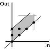
Figure 3: Exact and approximated fixed point

An approximation of the solutions of $w(\mathcal{M}_{1},\mathcal{M}_{2},\mathcal{M}_{3},x<2,x=x+1)$ is given by:

$$Q = P^{3}(x_{1},x_{3})\land x_{3}\geq 2$$

$$= x_{3}\geq 2\land x_{3}\leq 4\land x_{1}\leq x_{3}\land x_{1}\leq 3\land x_{1}\geq x_{3}-2$$

On the Polyhedral domain, convergence of the fixed point computation over $w(\mathcal{M}_{1},\mathcal{M}_{2},\mathcal{M}_{3},x<2,x=x+1)$ can be enforced by using widening techniques. The computation of $P^{k+1}$ is modified in order to use a widening operator $\nabla$ [12]. Thus, we have:

$$P^{k+1} = P^{k}(Init,Out)\nabla(P^{k}\land\alpha_{poly}(w(\mathcal{M}_{1},\mathcal{M}_{2},\mathcal{M}_{3},Dec,Body)))$$

A concrete algorithm for computing this approximation is given in [15], which permits to build implementation of $w$ in a constraint solver. As rooted in the Abstract Interpretation domain, the relation $w$ inherits from some of its fundamental correctness results, i.e., soundness and termination. However, it is worth pinpointing some differences.

Usually, a convex abstract polyhedron denotes the set of linear relations that hold over variables at a given point of a sequential program under analysis. As the goal here is to correctly approximate the set of solutions of a w relation, the polyhedron describes relations between input and output values and, thus, they involve more variables in the equations. In Abstract Interpretation, the analysis can be performed only once, whereas, in the case of the $w$ relation, the $join$ operation is launched everytime the relation is awaked without being succesfull in solving one of the guarded-constraint. As a consequence, we found out that it was not reasonable to use standard libraries to compute over polyhedra, such as PPL [3], because they use a dual representation for Polyhedra, which is a source of exponential time computations for the conversion.

4.5 Illustrative example

Looking at an iterative computation over unbounded domains as a relation captured by a $w$ constraint operator is interesting for adressing Constraint-Based Reacheability problems. On the one hand, the suspension mechanism offered by constraint reasoning allows us to cope with the approximation problem, i.e., the set of states that is considered is determined by the informations existing in the constraint store, which makes the reasoning more accurate w.r.t. the property to be demonstrated. On the other hand, adding abstract domain computations to the $w$ relation allows us to increase the level of deductions that can be achieved at each awakening of the $w$ constraint operator. To illustrate this remark, consider the following $C$ program:

f(  int i, ...  )  {
a.    j = 100;
b.      while( i > 0)
c.        { j=j+1 ; i=i-1 ;}
d.      ...
e.Ψif( j > 500)
f.Ψ    ...

A typical reachability problem is to find out a value of i such that statement f. is executed. Existing approaches for solving this reachability problem consider a path passing through f., e.g., a-b-d-e-f, and try to solve the path condition attached to this path. In this case, it means extracting constraint $j_{1}=100\land i_{1}\leq 0\land j_{1}>500$ and solving it to show that the constraint system is unsatisfiable, i.e., the corresponding path is infeasible. Then, these approaches backtrack to select another path (e.g., a-b-c-b-d-e-f with path condition $j_{1}=100\land i_{1}>0\land j_{2}=j_{1}+1\land i_{2}=i_{1}-1\land i_{2}\leq 0\land j_{2}>500$) and repeat the process again, until a satisfiable path condition is found. This example is pathologic for these approaches, as only the paths that iterate more than $400$ times in the loop will reach statement f.. Hopefully, using the constraint operator $w(\mathcal{M}_{1},\mathcal{M}_{2},\mathcal{M}_{3},i>0,j=j+1\land i=i-1)$ permits us to unrool dynamically $400$ times the loop without backtracking. The relational analysis performed on the Polyhedral abstract domain by the $w$ operator determines that $j_{out}-i_{in}=100$ whatever be the number of loop unrollings. Here, combining precise constraint reasoning in the concrete domain, with constraint extrapolation through abstract domain computations, offers us an efficient way of solving reachability problems on infinite-state systems.

5 Conclusions

In this paper, we have presented Constraint-Based Reachability as a process to combine constraint reasoning and abstraction techniques for solving reachability problems in infinite-state systems. The contribution is two-fold: first, we have revisited constraint consistency-filtering techniques by the prism of abstract domain computations ; second, we explained how to introduce abstract domain computation within the $w$ constraint operator reasoning. We have illustrated these notions with several examples in order to ease the understanding of the reader.

This appraoch has been implemented and tested on several problems, including real-world programs [20, 21]. The goal is now to broader the scope of these techniques that combine constraint reasoning and abstraction techniques, to adress fundamental problems such as reachability in infinite-state systems.

Appendix

This appendix contains the proofs of some of the results stated in the paper.

Theorem 9

Let $p$ be a filtering operator associated with constraint $c_{i}$, then $p$ computes domain-consistency iff $p=f_{i\_arc}^{\sharp}$.

Proof 1

($\Leftarrow$) Let $S_{1}=(f_{i}\circ\gamma_{arc})(S)$. From the definitions of $f_{i}$ and $\gamma$, we get that $S_{1}$ is the solution set of constraint $c_{i}$, given the initial domains $S$ (we write $S_{1}=sol(c_{i},S)$). Hence, $S^{\prime}=\alpha_{arc}(S_{1})=(A_{1},\ldots,A_{m})$ with
$A_{k}=\{x_{k}\leavevmode\nobreak\ |\leavevmode\nobreak\ x\in sol(c_{i},S)\}$. So, $c_{i}$ computes domain-consistency.
($\Rightarrow$) Let $p$ be a domain-consistency filtering operator. Suppose that there exists $S$ such that $p(S)=(A_{1},\ldots,A_{m})$ be strictly greater than $f_{i\_arc}^{\sharp}(S)=(B_{1},\ldots,B_{m})$. Then, there exists at least one $k$ such as $A_{k}\supsetneq B_{k}$. Hence, there exists an element $x_{k}$ of $A_{k}$ that does not belong to any solution of constraint $c_{i}$. Hence, $p$ cannot computes domain-consistency which is contradictory with the hypothesis. On the other side, $p$ cannot be smaller than $f_{i\_arc}^{\sharp}$ as it means that the filtering operator removes solutions. Hence, if $p$ computes domain-consistency then $p=f_{i\_arc}^{\sharp}$. $\Box$

Theorem 10

If $p$ is a filtering operator associated to constraint $c_{i}$, then $p$ computes bound-consistency iff $p=f_{i\_bound}^{\sharp}$.

Proof 2

($\Leftarrow$) From theorem 9, given initial intervals $I$, the domains $f_{i\_arc}^{\sharp}\circ\gamma_{inter}(I)$ are domain-consistent for constraint $c_{i}$. Applying function $\alpha_{inter}$ is similar to the process that keeps extremal values of each element of $f_{i\_arc}^{\sharp}\circ\gamma_{inter}(I)$. Hence, the resulting intervals satisfy the bound-consistency property.
($\Rightarrow$) (similar to the proof of theorem 9) If the filtering operator $p$ is greater than $f_{i\_bound}^{\sharp}$, then the computed intervals contain at least one bound that is not part of a solution of $c_{i}$, violating so the bound-consistency property. On the contrary, by supposing that $p$ is smaller than $f_{i\_bound}^{\sharp}$ then solutions are lost and $p$ is no more a filtering operator. Hence, if $p$ is a filtering operator guaranteeing bound-consistency then $p=f_{i\_bound}^{\sharp}$. $\Box$

References

- [1]
- [2] K. Apt (1999): The Essence of Constraint Propagation. Theoretical Computer Science 221(1-2), pp. 179–210, 10.1016/S0304-3975(99)00032-8.
- [3] Roberto Bagnara, Elisa Ricci, Enea Zaffanella & Patricia M. Hill (2002): Possibly Not Closed Convex Polyhedra and the Parma Polyhedra Library. In Springer, editor: SAS’02: In M. V. Hermenegildo and G. Puebla, editors, Proc. of the Static Analysis Symposium, LNCS 2477, pp. 213–229, 10.1007/3-540-45789-5_17.
- [4] S. Bardin & P. Herrmann (2011): OSMOSE: Automatic Structural Testing of Executables. Software Testing, Verification and Reliability (STVR) 21(1), pp. 29–54, 10.1002/stvr.423.
- [5] Peter Boonstoppel, Cristian Cadar & Dawson Engler (2008): RWset: Attacking path explosion in constraint-based test generation. In: Int. Conference on Tools and Algorithms for the Constructions and Analysis of Systems (TACAS’08), pp. 351–366, 10.1007/978-3-540-78800-3_27.
- [6] B. Botella, A. Gotlieb & C. Michel (2006): Symbolic execution of floating-point computations. The Software Testing, Verification and Reliability journal 16(2), pp. pp 97–121, 10.1002/stvr.333.
- [7] Richard H. Carver (1996): Testing abstract distributed programs and their implementations: A constraint-based approach. Journal of Systems and Software 33(3), pp. 223–237, 10.1016/0164-1212(96)00024-6.
- [8] F. Charreteur, B. Botella & A. Gotlieb (2009): Modelling dynamic memory management in Constraint-Based Testing. The Journal of Systems and Software 82(11), pp. 1755–1766. Special Issue: TAIC-PART 2007 and MUTATION 2007, 10.1016/j.jss.2009.06.029.
- [9] F. Charreteur & A. Gotlieb (2010): Constraint-Based Test Input Generation for Java Bytecode. In: Proc. of the 21st IEEE Int. Symp. on Softw. Reliability Engineering (ISSRE’10), San Jose, CA, USA, 10.1109/ISSRE.2010.26.
- [10] Chiu Wo Choi, Warwick Harvey, J. H. M. Lee & Peter J. Stuckey (2006): Finite Domain Bounds Consistency Revisited. In: Australian Conference on Artificial Intelligence, pp. 49–58, 10.1007/11941439_9.
- [11] P. Cousot & R. Cousot (1977): Abstract Interpretation : A unified lattice model for static analysis of programs by construction or approximation of fixpoints. In: Proceedings of Symp. on Principles of Programming Languages, ACM, pp. 238–252, 10.1145/512950.512973.
- [12] P. Cousot & N. Halbwachs (1978): Automatic Discovery of Linear Restraints Among Variables of a Program. In: Proceedings of Symp. on Principles of Programming Languages, ACM, pp. 84–96, 10.1145/512760.512770.
- [13] Patrick Cousot & Radhia Cousot (1976): Static Determination of dynamic properties of programs. In: Proc. of the 2nd International Symp. on Programming, Dunod, pp. 106–130.
- [14] Giorgio Delzanno & Andreas Podelski (2001): Constraint-based deductive model checking. International Journal on Software Tools for Technology Transfer (STTT) 3(3), pp. 250–270, 10.1007/s100090100049.
- [15] T. Denmat, A. Gotlieb & M. Ducasse (2007): An Abstract Interpretation Based Combinator for Modeling While Loops in Constraint Programming. In: Proceedings of Principles and Practices of Constraint Programming (CP’07), Springer Verlag, LNCS 4741, Providence, USA, pp. 241–255, 10.1007/978-3-540-74970-7_19.
- [16] T. Denmat, A. Gotlieb & M. Ducasse (2007): Improving Constraint-Based Testing with Dynamic Linear Relaxations. In: 18th IEEE International Symposium on Software Reliability Engineering (ISSRE’ 2007), Trollh ttan, Sweden, 10.1109/ISSRE.2007.12.
- [17] Cormac Flanagan (2004): Automatic software model checking via constraint logic. Sci. Comput. Program. 50(1-3), pp. 253–270. Available at http://dx.doi.org/10.1016/j.scico.2004.01.006.
- [18] Gordon Fraser & Franz Wotawa (2007): Test-Case Generation and Coverage Analysis for Nondeterministic Systems Using Model-Checkers. In: ICSEA, p. 45, 10.1109/ICSEA.2007.71.
- [19] P. Godefroid, N. Klarlund & K. Sen (2005): DART: directed automated random testing. In: Proc. of PLDI’05, pp. 213–223, 10.1145/1064978.1065036.
- [20] A. Gotlieb (2009): EUCLIDE: A Constraint-Based Testing platform for critical C programs. In: 2th IEEE International Conference on Software Testing, Validation and Verification (ICST’09), Denver, CO, 10.1109/ICST.2009.10.
- [21] A. Gotlieb (2012): TCAS software verification using Constraint Programming. The Knowledge Engineering Review 27(3), pp. 343–360, 10.1017/S0269888912000252.
- [22] A. Gotlieb, B. Botella & M. Rueher (1998): Automatic Test Data Generation Using Constraint Solving Techniques. In: Proc. of Int. Symp. on Soft. Testing and Analysis (ISSTA’98), pp. 53–62, 10.1145/271771.271790.
- [23] A. Gotlieb, B. Botella & M. Rueher (2000): A CLP Framework for Computing Structural Test Data. In: Proceedings of Computational Logic (CL’2000), LNAI 1891, London, UK, pp. 399–413, 10.1007/3-540-44957-4_27.
- [24] A. Gotlieb, T. Denmat & B. Botella (2005): Constraint-based test data generation in the presence of stack-directed pointers. In: 20th IEEE/ACM International Conference on Automated Software Engineering (ASE’05), Long Beach, CA, USA. 4 pages, 10.1145/1101908.1101958.
- [25] A. Gotlieb, T. Denmat & B. Botella (2007): Goal-oriented test data generation for pointer programs. Information and Soft. Technol. 49(9-10), pp. 1030–1044, 10.1016/j.infsof.2006.10.016.
- [26] T. Henzinger, R. Jhala, R. Majumdar & G. Sutre (2003): Software verification with Blast. In: Proc. of 10th Workshop on Model Checking of Software (SPIN), pp. 235–239, 10.1007/3-540-44829-2_17.
- [27] K. Marriott & P.J. Stuckey (1998): Programming with Constraints : An Introduction. The MIT Press.
- [28] R.A. Moore (1966): Interval Analysis. Prentice Hall, New Jersey.
- [29] M.N. Wegman & F.K. Zadeck (1991): Constant Propagation with Conditional Branches. ACM Transactions on Programming Language and Systems 13(2), pp. 181–210, 10.1145/103135.103136.
- [30] N. Williams, B. Marre, P. Mouy & M. Roger (2005): PathCrawler: Automatic Generation of Path Tests by Combining Static and Dynamic Analysis. In: Proc. Dependable Computing - EDCC’05, 10.1007/11408901_21.