Dynamic equivalences in the Hard-sphere Dynamic Universality Class

Abstract

We perform systematic simulation experiments on model systems with soft-sphere repulsive interactions to test the predicted dynamic equivalence between soft-sphere liquids with similar static structure. For this we compare the simulated dynamics (mean squared displacement, intermediate scattering function, $\alpha$-relaxation time, etc.) of different soft-sphere systems, between them and with the hard-sphere liquid. We then show that the referred dynamic equivalence does not depend on the (Newtonian or Brownian) nature of the microscopic laws of motion of the constituent particles, and hence, applies independently to colloidal and to atomic simple liquids. Finally, we verify another more recently-proposed dynamic equivalence, this time between the long-time dynamics of an atomic liquid and its corresponding Brownian fluid (i.e., the Brownian system with the same interaction potential).

I Introduction

At first sight, the macroscopic dynamics of supercooled liquids seems to be strongly material-specific, with no universal character at all. This is evidenced, for example, by the great diversity of molecular glass formers (ionic, metallic, organic, polymeric, etc.), giving rise to an overwhelmingly rich phenomenology ngaireview1 ; angellreview1 ; edigerreview1 ; angell ; debenedetti . One can easily understand this lack of universal behavior in terms of the wide differences in the materials’ structure and composition, the masses of their individual atoms, their preparation protocol, etc. Of course, the scenario becomes even more complex when one attempts to include colloidal systems in the discussion.

The formation of colloidal glasses and gels has been the subject of intense study during the last two decades sciortinotartaglia , and it is a widespread notion that the phenomenology of both, the glass transition in “thermally-driven” molecular glass formers, and the dynamic arrest transition in “density-driven” hard-sphere colloidal systems, might share a common underlying universal origin jammingrheology . Two relevant conceptual issues, however, must be understood in order for this expectation to have a more fundamental basis. The first one requires us to spell out the manner in which undercooling an atomic liquid might be equivalent to overcompressing a colloidal liquid. The second is to clarify under what conditions the macroscopic dynamics of both classes of systems could be expected to be equivalent, given the fact that the microscopic dynamics is Newtonian in atomic liquids and Brownian in colloidal fluids.

The answer to these two questions is highly relevant since it will allow us to understand which aspects of the macroscopic dynamics of a given system are universal and which ones are system-specific. These two issues have been addressed using computer simulation methods on well defined model systems. For example, interesting scalings of the equilibrium dynamics of simple models of soft-sphere glass formers have been exposed by systematic computer simulations xu ; berthierwitten1 , which provide an initial clue to the possible physical origin of the equivalence between the process of cooling and the process of compression. Similarly, also using computer simulations, it has been partially corroborated that standard molecular dynamics will lead to essentially the same dynamic arrest scenario as Brownian dynamics for a given model system (i.e., same pair potential) lowenhansenroux ; szamelflenner ; puertasaging .

From the theoretical side it would be desirable to have a unified description of the macroscopic dynamics of both, colloidal and atomic liquids, which explicitly predicts the aspects of the macroscopic dynamics that are expected to be universal. These topics might be addressed in the framework of a theory such as the mode coupling theory of the ideal glass transition goetze1 . In fact, the similarity of the long-time dynamics of Newtonian and Brownian systems in the neighborhood of the glass transition, for example, has been studied within this theoretical framework szamellowen . A number of issues, however, still remain open szamelflenner ; dyrejpcm2013 .

The present paper is part of an effort aimed at addressing these two fundamental issues within a general theoretical framework, namely, the generalized Langevin equation (GLE) formalism boonyip ; delrio ; faraday . This formalism was employed in the construction of the self-consistent generalized Langevin equation (SCGLE) theory of colloid dynamics scgle0 ; scgle1 ; scgle2 , eventually applied to the description of dynamic arrest phenomena rmf ; todos1 ; todos2 , and more recently, to the construction of a first-principles theory of equilibration and aging of colloidal glass-forming liquids noneqscgle0 ; noneqscgle1 .

When applied to model systems with soft repulsive interactions soft1 , the SCGLE theory of colloid dynamics, together with the condition of static structural equivalence between soft- and hard-sphere systems, predicts the existence of a “hard-sphere dynamic universality class”, constituted by the soft-sphere systems whose dynamic parameters, such as the $\alpha$-relaxation time and self-diffusion coefficient, depend on density, temperature and softness in a universal scaling fashion soft2 , through an effective hard-sphere diameter determined by the Andersen-Weeks-Chandler awc ; hansen criterion. These predictions provide a more fundamental explanation of the scalings previously exhibited by computer simulations xu ; berthierwitten1 , and point to the physical basis of the dynamic equivalence between cooling and compressing.

The main purpose of this paper is to report the results of, and to provide detailed technical information on, a number of simulation experiments performed with the purpose of testing this density-temperature-softness scaling in the referred dynamic universality class. An illustrative selection of these results were advanced in a recent brief communication soft2 . The second main purpose of the present paper is to perform the pertinent simulation experiments to test a second relevant prediction of the SCGLE theory, which addresses the second of the two fundamental issues mentioned above, namely, the macroscopic dynamic equivalence between atomic and colloidal liquids. As it happens, the SCGLE theory of colloid dynamics is being extended to describe the dynamics of simple atomic liquids atomic1 ; atomic2 . The scenario that emerges from these theoretical developments include well defined scaling rules that exhibit the equivalence between the dynamics of colloidal fluids and the long-time dynamics of atomic liquids. Here we test these scalings by comparing the simulation results for a given model system using both, molecular dynamics and Brownian dynamics simulations.

Thus, the present paper is essentially a report of a set of systematic computer simulations. In Sec. II we define the model systems considered in our study and provide the basic information on the simulation methods employed. In Sec. III we review the concept of static structural equivalence between soft- and hard-sphere fluids, and explain how this concept is employed to map the static structure of any soft-sphere liquid onto the properties of an effective hard-sphere liquid. In Sec. IV we review the extension of this structural equivalence to the dynamic domain and present the simulation results that validate the accuracy of the resulting dynamic equivalence between soft- and hard-sphere liquids. We first verify that this dynamic equivalence is exhibited by our Brownian dynamics simulations, and then confirm that the same dynamic equivalence is also observed in the results of our molecular dynamics simulations. In Sec. V we explain the correspondence between the dynamics of colloidal fluids and the long-time dynamics of atomic liquids, and verify that the predicted scalings are indeed satisfied by our molecular and Brownian dynamics simulations. In the last section, Sec. VI, besides summarizing the main results of this paper, we explain that for the systems with interaction potential in the hard sphere dynamic universality class, these effects can be taken into account through the value of the short-time self-diffusion coefficient, thus expanding the applicability of the scalings discussed here. At this point we have to mention that the present study only involves Brownian dynamics simulations that completely ignore the effects of hydrodynamic interactions, which have an enormous practical relevance in concentrated colloidal fluids.

II Methodological aspects

In this section we describe the most relevant methodological aspects of this work. This includes information on the numerical simulation methods and on the theoretical concepts and approaches employed.

II.1 Model potentials

Let us consider a model liquid formed by N spherical particles in a volume V which interact through a soft repulsive pair potential $u(r)$ with tunable softness. We intend to study the interplay of the effects of the number density (or concentration, in the case of colloidal liquids) $n\equiv N/V$, temperature $T$, and softness, represented by some parameter denoted generically as $\nu$. There is a variety of analytic proposals for such tunable soft potential xu ; berthierwitten1 , but for concreteness here we shall refer explicitly to three specific representative model systems. The first is the truncated Lennard-Jones (TLJ) potential,

$$u^{(\nu)}(r)=\epsilon\left[\left(\frac{\sigma}{r}\right)^{2\nu}-2\left(\frac{\sigma}{r}\right)^{\nu}+1\right]\Theta(\sigma-r),$$ (1)

in which $\Theta(x)$ is the unit step function. The positive parameter $\nu$ controls the softness of the interaction, with the limit $\nu\to\infty$ corresponding to the hard sphere potential between particles of diameter $\sigma$. For fixed $\nu$, the state space of this system is spanned by the dimensionless temperature $T^{*}\equiv k_{B}T/\epsilon$ and volume fraction $\phi=\pi n\sigma^{3}/6$.

The second representative model system we shall refer to is the inverse power-law (IPL) potential

$$u(r)=\epsilon(\sigma/r)^{2\nu},$$ (2)

commonly used to model hard sphere effects. Just like in the case of the TLJ model, for fixed softness parameter $\nu$ the state space of the IPL model system is also spanned by the dimensionless temperature $T^{*}\equiv k_{B}T/\epsilon$ and volume fraction $\phi=\pi n\sigma^{3}/6$. The fundamental difference between the IPL potential and the TLJ interaction is that the latter is always short-ranged.

The third interaction model that we shall refer to is defined by the hard-sphere plus repulsive Yukawa (HSY) potential, frequently used to model the screened electrostatic repulsions between charged colloidal particles nagele0 . This is defined here as

$$u(r)=\epsilon\left[\frac{\exp[-z(r/\sigma-1)]}{(r/\sigma)}\right].$$ (3)

For fixed screening parameter $z$, the state space of this system is also spanned by the volume fraction $\phi=\pi n\sigma^{3}/6$ and the dimensionless temperature $T^{*}\equiv k_{B}T/\epsilon$ (sometimes, however, we shall also refer to the repulsion intensity parameter $K\equiv 1/T^{*}=\beta\epsilon$). The inverse screening length $z$ controls the range of the potential, and for our purpose, we may consider that it plays the role of the softness parameter. Typical values for these parameters representing real suspensions of highly charged colloidal suspensions at low ionic strength in the dilute regime are $K=554$, $z=0.149$, and $\phi$ of the order of $10^{-4}$ gaylor . We shall use these as illustrative values, along with $K=100$ and $z=1.0$. Figure 1 plots these interaction models for some specific values of these parameters to illustrate the variety of interactions considered.

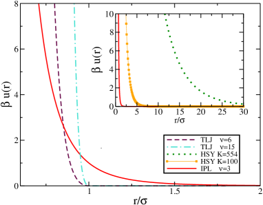
Figure 1: Illustration of the truncated Lennard-Jones (TLJ), inverse power-law (IPL), with $T^{*}=1$ and hard-sphere plus repulsive Yukawa (HSY) potentials, with $K=100$ and $K=554$.

II.2 Simulations

Molecular dynamics (MD) simulations using the velocity-verlet algorithm allen were conducted for the model liquids above, formed by N spherical particles of mass $M$ in a simulation box of volume V. The results are expressed in the well known Lennard-Jones units, where $M$, $\sigma$ and $\epsilon$ are taken as the units of mass, length, and energy, respectively, and $t_{MD}=\sqrt{M\sigma^{2}/k_{B}T}$ is the corresponding time unit.

For Brownian dynamics (BD) simulations we follow the prescription proposed by Ermak and McCammon allen to evolve the positions of the particles in the simulation box. Thus, a given particle at position $\vec{r}(t)$ and under the force $\vec{F}(t)$ is displaced in the $\alpha$ direction according to

$$r_{\alpha}(t+\Delta t)=r_{\alpha}(t)+\beta D^{0}F_{\alpha}(t)\Delta t+R_{\alpha}$$ (4)

where $D^{0}$ is the short-time self-diffusion coefficient, $\Delta t$ is the time step, and $R_{\alpha}$ is a random displacement extracted from a Gaussian distribution with zero mean and variance $2D^{0}\Delta t$. Taking $\sigma$ as the length unit and $\epsilon$ as the energy unit, $t_{BD}\equiv\sigma^{2}/D^{0}$ becomes the natural time unit.

In both cases, the simulations were conducted with $N=1000$ particles in a cubic simulation box with periodic boundary conditions. The initial configurations were generated using the following procedure. First, particles were placed randomly in the simulation box at the desired density, such that the maximum overlap between particles was in the range $0.65\sigma-0.8\sigma$. To relax this initial configuration and reduce or eliminate the overlap between the particles we tried two methods. In one of them we perform Monte Carlo cycles swapmc at a high temperature, and then decrease the temperature for several steps until the original temperature was restored. In the other method we uniformly expand the system by increasing the length of the simulation box by a factor of at least $1.5$. Then, we run MD or MC cycles while decreasing the simulation box until the original value was reached. We checked that the these two methods produce equivalent results. Once the initial configuration is constructed, several thousand cycles are performed to lead the systems to equilibrium, followed by at least two million cycles where the data is collected. In the case of MD simulations, temperature was kept constant by simple rescaling of the velocities of the particles every 100 time steps allen .

Several structural and dynamic properties are calculated from the equilibrium configurations generated in the simulations. In particular, the radial distribution function $g(r)$ was calculated using the standard approach allen . The static structure factor $S(k)$ can then be obtained as

$$S(k)=1+4\pi n\int[g(r)-1]\frac{\sin(kr)}{kr}r^{2}dr.$$ (5)

Alternatively, $S(k)$ can be calculated directly from the positions of the particles in the simulation box hansen .

Time correlation functions, like the mean squared displacement (MSD)

$$W(t)=\left<(\Delta\vec{r}(t))^{2}\right>/6,$$ (6)

and the self-intermediate scattering function $F_{S}(k,t)$,

$$F_{S}(k,t)=\left<\frac{1}{N}\sum_{j=1}^{N}\exp(-i\vec{k}\cdot\vec{\Delta}r_{j}(t))\right>,$$ (7)

where $\Delta\vec{r}_{j}=\vec{r}_{j}(t)-\vec{r}_{j}(0)$, were calculated using the efficient, low-memory algorithm proposed in Ref. wdtblocks .

Crystallinity of the systems was monitored through the order parameters $Q_{l}$, especially $Q_{6}$, defined as

$$Q_{l}=\left[\frac{4\pi}{2l+1}\sum_{m=-l}^{l}|Q_{lm}|^{2}\right]^{1/2},$$ (8)

where $Q_{lm}$ is basically the average, over all particles, of the mean spherical harmonics $Y_{lm}(\hat{r}_{ij})$ established between each particle $i$ and its close neighbors ($j=1,...,N_{b}(i)$), where $N_{b}(i)$ is the number of neighbors of the particle qls . Since in this paper we are interested only in the amorphous liquid state, when the simulations of monodisperse systems exhibited crystalline order, thus indicating that the corresponding volume fraction was beyond the freezing point, we discarded that monodisperse run, and performed an alternative simulation introducing size polydispersity to frustrate crystallization. Polydispersity is handled following previous work gabriel , where the diameters of the $N$ particles are taken to be evenly distributed between $\bar{\sigma}(1-w/2)$ and $\bar{\sigma}(1+w/2)$, with $\bar{\sigma}$ being the mean diameter. We consider the case $w=0.3$, corresponding to a polydispersity $P=w/\sqrt{12}=0.0866$. Let us emphasize that this procedure was followed in both, molecular and Brownian dynamics simulations, and that in both cases only size polydispersity was introduced, leaving all the other parameters unchanged (such as the mass or the short-time self-diffusion coefficient of the particles).

At this point, it is important to emphasize that when the system remains in its metastable liquid phase, the equilibration time increases enormously as the system approaches its dynamic arrest transition (see the detailed discussion in Ref. gabriel ). This means that as the volume fraction increases in the metastable region, the initial equilibration period will eventually be insufficient, and will need to be adjusted to make sure that the system indeed equilibrated properly, as recommended in gabriel . The present study, however, is not aimed at studying the equilibration process by itself, and hence, we shall avoid approaching too closely the actual glass transition, so as to focus our attention on the subject of this work, namely, on the dynamic equivalence between soft-sphere liquids.

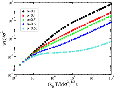
Figure 2: MSD from MD simulations TLJ systems with $\nu=15$, $T^{*}=1$, and the volume fraction $\phi=0.1,0.4,0.5,0.6$, and 0.65. The most concentrated sample ($\phi=0.65$) is polydisperse.

To illustrate the end result of this procedure, in Fig. 2 we show the corresponding MSD for TLJ system with $\nu=15$ at $T^{*}=1$ for volume fractions $\phi=0.1,0.4,0.5,0.6,0.65$. These results fully cover the stable fluid phase, with the metastable liquid regime represented by the polydisperse system with volume fraction $\phi\equiv V^{-1}\sum_{i=1}^{N}\pi\sigma_{i}^{3}/6=0.65$ (whose monodisperse counterpart is already highly ordered). In all samples the MSD clearly exhibits the ballistic and diffusive time regimes typical of atomic liquids.

III Soft-hard static equivalence

Although simulations are the main methodology employed here to generate the static and the dynamic information of the model systems above, the analysis of this information will rely on a few theoretical notions, most notably the predicted static and dynamic equivalence between soft-sphere and hard-sphere liquids. In this analysis, however, we shall recurrently need the exact structural properties of the fluid of hard-spheres of diameter $\sigma$ and volume fraction $\phi$, embodied in its RDF $g_{HS}(r/\sigma;\phi)$ or in its static structure factor $S_{HS}(k\sigma;\phi)$. For these structural properties a virtually exact representation is provided by the Percus-Yevick (PY) percusyevick ; wertheim approximation with its Verlet-Weis correction, defined as verletweis

$$g_{HS}(r/\sigma;\phi)=g^{(PY)}(r/\sigma_{w};\phi_{w}),$$ (9)

and

$$S_{HS}(k\sigma;\phi)=S^{(PY)}(k\sigma_{w};\phi_{w}),$$ (10)

with the parameters $\phi_{w}$ and $\sigma_{w}$ defined as

$$\phi_{w}\equiv\phi-\phi^{2}/16,$$ (11)

and

$$\sigma_{w}\equiv\sigma(\phi_{w}/\phi)^{1/3}.$$ (12)

The functions $g^{(PY)}(x;\phi)$ and $S^{(PY)}(y;\phi)$ are the solution of the Ornstein-Zernike equation with PY closure for the HS fluid provided, for example, by Wertheim wertheim as easily programmable analytic expressions. The resulting $g_{HS}(r/\sigma;\phi)$ will be employed recurrently in the practical implementation of the concept of static structural equivalence between soft- and hard-sphere systems. This notion was first introduced as an essential aspect of the equilibrium perturbation theory of liquids awc ; verletweis ; hansen .

The equilibrium static structure of the generic soft-sphere system of the type discussed here is represented by the radial distribution function (RDF) $g(r;n,T;\sigma,\epsilon,\nu)$, also written in terms of dimensionless variables as $g(r/\sigma;\phi,T^{*},\nu)$, with $T^{*}\equiv k_{B}T/\epsilon$ and $\phi=\pi n\sigma^{3}/6$. The physical notion behind the principle of static equivalence is that at any state point $(\phi,T^{*},\nu)$, this soft-sphere system is structurally identical to a hard-sphere system with a state-dependent effective hard-sphere diameter $\sigma_{HS}$ and effective number density $n_{HS}$. This means that for any state point $(\phi,T^{*},\nu)$ one can find a diameter $\sigma_{HS}=\sigma_{HS}(\phi,T^{*},\nu)$ and a number density $n_{HS}=n_{HS}(\phi,T^{*},\nu)$ such that $g(r;n,T;\sigma,\epsilon,\nu)\approx g_{HS}(r;n_{HS},\sigma_{HS})$, where $g_{HS}(r;n_{HS},\sigma_{HS})$ is the radial distribution function of the HS system, also written as $g_{HS}(r/\sigma_{HS};\phi_{HS})$, with $\phi_{HS}=\pi n_{HS}\sigma_{HS}^{3}/6$. This condition for structural equivalence can thus be written in terms of dimensionless variables as

$$g\left(\frac{r}{\sigma};\phi,T^{*},\nu\right)\approx g_{HS}(\frac{r}{\sigma_{HS}};\phi_{HS}),$$ (13)

with

$$\phi_{HS}=\frac{\pi}{6}n_{HS}\sigma_{HS}^{3}=\lambda_{n}\lambda_{\sigma}^{3}\phi,$$ (14)

where $\lambda_{\sigma}$ is just the state-dependent effective hard-sphere diameter in units of $\sigma$,

$$\lambda_{\sigma}(\phi,T^{*},\nu)\equiv\sigma_{HS}(\phi,T^{*},\nu)/\sigma,$$ (15)

and $\lambda_{n}$ is the state-dependent HS particle number density in units of $n$,

$$\lambda_{n}(\phi,T^{*},\nu)\equiv n_{HS}(\phi,T^{*},\nu)/n.$$ (16)

Thus, the condition for structural equivalence can be written in scaled form as

$$g\left(\frac{r}{\sigma};\phi,T^{*},\nu\right)\approx g_{HS}\left(\lambda_{\sigma}^{-1}\frac{r}{\sigma};\lambda_{n}\lambda_{\sigma}^{3}\phi\right).$$ (17)

This equivalence condition can be used in several manners. The first one is to determine the parameters $\sigma_{HS}$ and $n_{HS}$ that correspond to a given soft-sphere system at a given state, i.e., to determine the functions $\sigma_{HS}=\sigma_{HS}(\phi,T^{*},\nu)$ and $n_{HS}=n_{HS}(\phi,T^{*},\nu)$. This might be done theoretically, using specific assumptions. For example, one could assume that $n_{HS}=n$ and that $\sigma_{HS}$ is $\phi$-independent, with $\sigma_{HS}=\sigma_{HS}(T^{*},\nu)$ determined by means of an approximate version of the equivalence condition in Eq. (13). For example, the approximation employed in the so-called blip-function method reads in general hansen

$$\int_{0}^{\infty}4\pi r^{2}\left[e^{-\beta u(r)}-e^{-\beta u_{HS}(r)}\right]dr=0,$$ (18)

which for the TLJ system can be written as

$$\lambda^{3}_{\sigma}(T^{*},\nu)=1-3\int_{0}^{1}dxx^{2}{\exp\left[-\frac{1}{T^{*}}(\frac{1}{x^{2\nu}}-\frac{2}{x^{\nu}}+1)\right]}.$$ (19)

Evaluating $\lambda_{\sigma}(T^{*},\nu)$ determines $\sigma_{HS}$ as $\sigma_{HS}(T^{*},\nu)=\sigma\lambda_{\sigma}(T^{*},\nu)$.

Naturally, this or any other approximate scheme has a limited range of validity. For example, as we shall see shortly, the blip function method is reasonably accurate for finite-range, moderately soft potentials, such as the TLJ liquid with softness parameter $\nu\gtrsim 6$, but it fails completely for systems with much softer and longer-ranged potentials, such as the HSY fluid with $K=554$, $z=0.149$, and $\phi$ of the order of $10^{-4}$. Thus, it is important to search for a more robust method to determine the functions $\sigma_{HS}=\sigma_{HS}(\phi,T^{*},\nu)$ and $n_{HS}=n_{HS}(\phi,T^{*},\nu)$.

One possible method, proposed in Ref. dynamicequivalence , is to determine the diameter $\sigma_{HS}=\sigma_{HS}(\phi,T^{*},\nu)$ and the number density $n_{HS}=n_{HS}(\phi,T^{*},\nu)$ of the HS system whose radial distribution function provides the best overall fit of the exact RDF $g(r;n,T;\sigma,\epsilon,\nu)$ of the soft-sphere liquid previously determined, for example, by computer simulations. This method is illustrated here in Fig. 3, where we plot simulation data for the RDF of three soft-sphere model potentials (TLJ, IPL, and HSY). Fig. 3(a), for example, plots the RDF $g(r/\sigma;\phi,T^{*},\nu)$ of the TLJ liquid with $\nu=6$, $T^{*}=1$, and $\phi=0.70$. Thus, we first determine the effective hard sphere volume fraction $\phi_{HS}$ by plotting the exact RDF $g_{HS}(r/\sigma;\phi_{HS})$ of Eq. (9) for various volume fractions until we identify the value of $\phi_{HS}$ such that the height of its second maximum matches the height of the second maximum of the soft sphere RDF ($\approx$ 1.37, indicated by the thin horizontal line in the figure). The solid curve is the resulting hard sphere RDF.

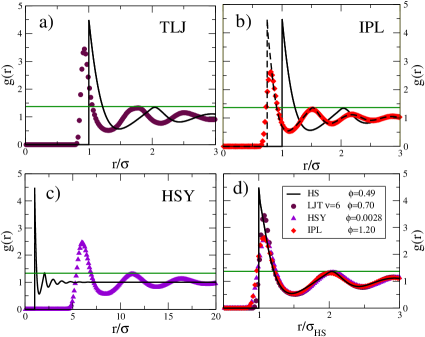
Figure 3: Radial distribution function for (a) a TLJ liquid with $\nu=6$, $T^{*}=1$, and $\phi=0.70$; (b) an IPL liquid with $\nu=3$, $T^{*}=1$; and $\phi=1.2$, and (c) a HSY liquid with $K=554$, $z=0.149$, and $\phi=2.8\times 10^{-3}$. All the systems share the same $\phi_{HS}=0.49$. Solid lines corresponds to the Percus-Yevick approximation for HS with the Verlet-Weis correction.

This procedure assigns a unique value of $\phi_{HS}$ to that set of values of the parameters $(\phi,T^{*},\nu)$, i.e., it determines the function $\phi_{HS}=\phi_{HS}(\phi,T^{*},\nu)$. As observed in figure (3a), the height of these two second maxima of $g(r)$ coincide, but their positions differ. One finds, however, that a simple linear rescaling $r\to\lambda_{\sigma}^{-1}r$ of the radial coordinate of this HS RDF, prescribed by the equivalence condition in Eq. (17), suffices to match the position of both second maxima. This rescaling determines the parameter $\lambda_{\sigma}$, and hence, also the effective hard-sphere diameter $\sigma_{HS}$ at the state point $(\phi,T^{*},\nu)$ as $\sigma_{HS}=\sigma\lambda_{\sigma}(\phi,T^{*},\nu)$. Finally, the function $n_{HS}=n_{HS}(\phi,T^{*},\nu)$ is determined by

$$n_{HS}=n\left(\frac{\phi_{HS}}{\phi}\right)\left(\frac{\sigma}{\sigma_{HS}}\right)^{3}.$$ (20)

Following this procedure, in the illustrative example in Fig. 3(a) we find $\phi_{HS}=0.49$ and $\lambda_{\sigma}=\sigma_{HS}/\sigma=0.88$; and therefore $\lambda_{n}=n_{HS}/n=1.01$. These numbers differ only slightly from the results of the blip function method, which assumes $\lambda_{n}=1$ and determines that $\lambda_{\sigma}=0.888$ and $\phi_{HS}=0.49$, a comparison that illustrates the accuracy of the blip function method for the TLJ potential with $\nu=6$. This accuracy improves for more rigid potentials and deteriorates for softer and longer-ranged ones.

For example, Fig. 3(b) reports an identical exercise for the IPL potential with $\nu=3$, $T^{*}=1$, and $\phi=1.2$, whose RDF is represented by the symbols in the figure. Here again the solid line is the RDF of the equivalent HS system as a function of $r/\sigma$ and the dashed line is the same RDF, but now plotted as a function of $r/\sigma_{HS}=\lambda_{\sigma}^{-1}r/\sigma$, to illustrate the overall agreement between the RDF of the soft-sphere system and that of the equivalent HS system. This method determines the effective HS parameters $\phi_{HS}=0.49$, $\lambda_{\sigma}=0.71$, and $\lambda_{n}=0.9679$. In contrast, the blip function method, which assumes $\lambda_{n}=1$, determines in this case the value $\lambda_{\sigma}=1.209$ and the unphysical HS volume fraction $\phi_{HS}=2.41$.

Finally, Fig. 3(c) reports the same exercise but for a much softer and longer-ranged interaction, namely, the HSY liquid with $K=554$, $z=0.149$, and $\phi=2.8\times 10^{-3}$. As before, the solid line is the RDF of the equivalent HS system as a function of $r/\sigma$. In this case, the resulting effective HS parameters are $\phi_{HS}=0.49$, $\lambda_{\sigma}=5.55$, and $\lambda_{n}=1.0036$. In contrast, the blip function method ($\lambda_{n}=n_{HS}/n=1$) determines the completely unphysical values $\lambda_{\sigma}=\sigma_{HS}/\sigma=27.6$ and $\phi_{HS}=63.4$. Thus, the first conclusion of these three illustrative examples is that the assumption that $\lambda_{n}\approx 1$, employed in the blip function method above, may indeed be a good approximation in the circumstances illustrated by these three examples corresponding to the HS liquid at $\phi_{HS}=0.49$. It is then the blip-function determination of the hard sphere diameter through Eq. (19) what is not an accurate prescription.

Let us mention that in each of the three cases corresponding to panels (a)-(c) of Fig. 3 we chose to plot the two equivalent RDFs as a function of the radial distance $r$ measured in the length unit $\sigma$ of the respective system. This comparison, however, can also be done using instead the effective HS diameter $\sigma_{HS}$ as the common unit length, as it is done in Fig. 3(d). There we note, in addition, that except for the shape of $g(r)$ near contact (which is highly system-specific), the simulation data of the three systems are actually coincident, and that we only have a single HS RDF, corresponding to $\phi_{HS}=0.49$ and represented by the solid line in Fig. 3(d). This coincidence illustrates another important feature, namely, that different soft-sphere systems that share the same static structure also share the same effective HS volume fraction.

This figure also illustrates the fact that the structural equivalence condition in Eq. (13) can also be used in an inverse manner, i.e., to identify the state of a given soft-sphere system whose structure matches the structure of a prescribed HS system. In reality, what we actually did for each of the three soft-sphere model systems in the examples in Fig. 3 was to search for the state whose structure matched the structure of the HS liquid with the prescribed volume fraction $\phi_{HS}=0.49$. For this we varied the soft-sphere density (or volume fraction $\phi$), keeping the temperature fixed, until meeting this condition.

In reality, the procedure just described to determine the equivalent hard sphere system of a given soft-sphere model is not limited to circumstances in which the condition $\lambda_{n}=n_{HS}/n\approx 1$ is satisfied, as in the last three examples. For example, if we consider again the same systems discussed in Fig. 3, but at states that correspond to effective hard-sphere volume fractions lower than $0.49$, the structural equivalence will have the same degree of accuracy as the examples in Fig. 3, even though the condition $n_{HS}\approx n$ may definitely no longer be satisfied. To illustrate the degree of the possible departures of the ratio $n_{HS}/n$ from unity, in Fig. 4 we plot $n_{HS}/n$ for the TLJ, IPL, and HSY models, not as a function of the respective volume fractions of each model system, but as a function of the effective HS volume fraction, which is a common indicator of the effective degree of packing of the three systems. There we see that the TLJ system, whose pair interaction is always short-ranged, virtually always satisfies the condition $\lambda_{n}=n_{HS}/n\approx 1$, whereas the largest departures from this condition are observed in the liquids with longer-ranged potentials, such as the IPL and HSY systems at low effective volume fractions.

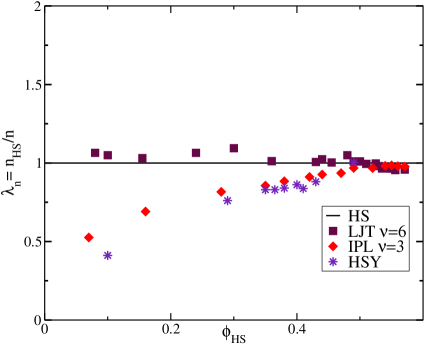
Figure 4: Ratio $n_{HS}/n$ as a function of the volume fraction of the equivalent HS systems for LJT, IPL and HSY.

Another important observation is that for the model interaction potentials employed in the present discussion, the height of the second maximum of the RDF is not the only simple structural order parameter. In reality, some other properties that derive from the general equivalence condition in Eq. (13) might serve as alternative structural order parameters. One of them is the main peak of the static structure factor $S(k)$, whose height $S_{max}$ allows us to determine $\phi_{HS}$, and whose rescaled position $k_{max}$ determines the effective HS diameter $\sigma_{HS}$. This is illustrated in Fig. 5, which exhibits the structure factors of the same systems as in the previous figure, plotted as a function, in one case of $k\sigma$ (insets) and in the other case of $k\sigma_{HS}$ (main figure).

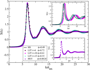
Figure 5: Static structure factors for the three soft-sphere systems of Fig. 3.

Since our study will include densities higher than the freezing density of the monodisperse fluid, we need to introduce polydispersity in our simulations and this requires us to adapt the previously-described procedure to polydisperse systems. Although polydispersity will not affect dramatically the most relevant dynamic properties, it happens to have a profound effect on the thermodynamic and structural properties, in particular on the height of the second peak of $g(r)$ and of the main peak of $S(k)$. These structural order parameters are found to decrease with polydispersity (for fixed volume fraction), and this requires us to adapt the method described above, to identify in a simple manner the effective hard-sphere system that corresponds to a given polydisperse soft-sphere liquid. The adapted procedure is the following. Consider a given soft-sphere system with (size) polydispersity $P$ and mean diameter $\sigma$, whose overall RDF $g(r/\sigma;\phi,T^{*},\nu)$ has been measured or simulated. Within a discretized representation the probability of having a diameter $\sigma_{i}$ ($i=1,2,...,\nu$) is $p(\sigma_{i})=x_{i}$, with $x_{i}=n_{i}/n$ being the molar fraction of species $i$. Under these circumstances $g(r/\sigma;\phi,T^{*},\nu)$ is defined as $g(r/\sigma;\phi,T^{*},\nu)\equiv\sum_{\alpha,\beta=1}^{\nu}\sqrt{x_{\alpha}x_{\beta}}g_{\alpha\beta}(r)$, with $g_{\alpha\beta}(r)$ being the partial radial distribution functions. As in the monocomponent case, determining the equivalent polydisperse hard-sphere system whose overall RDF $g_{HS}(r/\sigma_{HS};\phi_{HS})$ matches the simulated $g(r/\sigma;\phi,T^{*},\nu)$, leads to the determination of the total effective HS volume fraction $\phi_{HS}$ and the mean HS diameter $\sigma_{HS}$.

To implement this procedure we need to determine the partial RDFs of a multicomponent hard-sphere system at arbitrary total volume fraction $\phi_{HS}$, but constrained to have the same polydispersity $P$ as the soft-sphere system. For this, we represent the equivalent polydisperse HS system as an equi-molar binary mixture of hard spheres of diameters $\sigma_{1}=\sigma_{HS}(1-P)$ and $\sigma_{2}=\sigma_{HS}(1+P)$ with $\sigma_{HS}$ being the mean HS diameter. The overall RDF $g_{HS}(r)$ of this system is given by $g_{HS}(r)\equiv[g_{11}^{HS}(r)+2g_{12}^{HS}(r)+g_{22}^{HS}(r)]/2$, with $g_{\alpha\beta}^{HS}(r)$ being the corresponding partial RDFs, which are obtained from the analytic solution of the multicomponent Percus-Yevick approximation lebowitzhs2mixt ; hiroike , complemented again with the VW correction williamsvanmegen , i.e., $\phi_{HS}\to\phi_{w}$, with $\phi_{w}\equiv\phi_{HS}-\phi_{HS}^{2}/16$, as in Eqs. (9)-(12), with $\sigma$ and $\phi$ reading $\sigma_{HS}$ and $\phi_{HS}$. The resulting HS structure factors will be denoted as PY-VW. As in the monocomponent case, the RDF $g_{HS}(r;\phi_{HS})$ at arbitrary $\phi_{HS}$ is then compared with the soft-sphere simulation results until determining the value of $\phi_{HS}$ whose $g_{HS}(r;\phi_{HS})$ matches the height of the second peak of the simulated RDF of the polydisperse soft-sphere system.

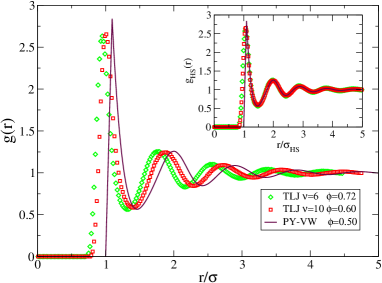
Figure 6: RDF’s for polydisperse systems, with $\nu=6$ and $\nu=15$ and $\phi_{HS}=0.5$. The line corresponds to the solution of the PY-VW theory for the corresponding HS systems. Inset: RDFs after scaling the radial distance.

We illustrate this structural equivalence using a polydisperse version of the TLJ model with different softness, $\nu=6$ and $\nu=15$, but with densities corresponding to the same effective HS volume fraction $\phi_{HS}=0.5$, and the same polydispersity $P=0.0866$ (which is large enough to inhibit the crystallization of hard spheres up to very high volume fractions gabriel ). Fig. 6 presents the simulation results for the total RDF $g(r/\sigma;\phi,T,\nu)$, along with the theoretical data for $g_{HS}(r;\phi_{HS})$ of the corresponding HS binary mixture. As we can observe in the inset, the scenario is quite similar to the one for monodisperse systems. Furthermore, this inset also reveals that using the effective HS diameter to scale the radial distance $r$ of the data in the main figure, collapses the radial distribution function of the two polydisperse soft-sphere systems onto each other. Thus, the results in Figs. 3 and 6 show that our protocol to determine the equivalent hard sphere system works very well in a wide range of volume fractions for both monodisperse and polydisperse systems. With this essential step covered, we now investigate its implications on the dynamics of structurally equivalent systems.

IV Soft-hard Dynamic Equivalence

The dynamic extension of the previous soft–hard static structural equivalence was discussed in Refs. dynamicequivalence ; soft1 in the context of the dynamics of Brownian liquids, in which a short-time self-diffusion coefficient $D^{0}$ describes the diffusive microscopic dynamics of the colloidal particles “between collisions”. The following discussion also refers to Brownian systems, but in the second part of this section we shall consider atomic liquids, whose short-time dynamics is ballistic.

IV.1 Brownian liquids

Although the dynamic equivalence we are about to discuss can probably be understood from several perspectives, our original insight and motivation derived from a straightforward prediction of the self-consistent generalized Langevin equation (SCGLE) theory of colloid dynamics. This theory can be summarized by a closed system of equations for the collective and self intermediate scattering functions $F(k,t)$ and $F_{S}(k,t)$ rmf ; todos1 ; todos2 , which in Laplace space read

$$F(k,z)=\frac{S(k)}{z+\frac{k^{2}D^{0}S^{-1}(k)}{1+m(k)\Delta\zeta^{*}(z)}},$$ (21)

and

$$F_{S}(k,z)=\frac{1}{z+\frac{k^{2}D^{0}}{1+m(k)\Delta\zeta^{*}(z)}},$$ (22)

with $D^{0}$ being the short-time self-diffusion coefficient. These equations become a closed system of equations when complemented with the following approximate expression for the time-dependent friction function $\Delta\zeta^{*}(t)$,

$$\Delta\zeta^{*}(t)=\frac{D^{0}}{3\left(2\pi\right)^{3}n}\int d{\bf k}\left[\frac{k[S(k)-1]}{S(k)}\right]^{2}F(k,t)F_{S}(k,t),$$ (23)

and with the following definition of the “interpolating” function $m(k)$ todos2

$$m(k)\equiv\frac{1}{1+\left(\frac{k}{k_{c}}\right)^{\mu}},$$ (24)

with $\mu=2$ and with $k_{c}$ being the empirically chosen cutoff wave-vector $k_{c}=1.118k_{max}$, with $k_{max}$ being the position of the main peak of $S(k)$.

From these equations and the condition for structural equivalence in Eq. (13), $g\left(r/\sigma;\phi,T^{*},\nu\right)\approx g_{HS}(r/\sigma_{HS};\phi_{HS})$, it is not difficult to see that when $\lambda_{n}=n_{HS}/n\approx 1$ (an excellent assumption in many circumstances, such as those illustrated in Fig. 3), the dimensionless properties $F(k,t)$, $F_{S}(k,t)$, and $\Delta\zeta^{*}(z)$ of a given soft-sphere system, can only depend on the wave-vector $k$ and the time $t$ through the dimensionless variables $k\sigma_{HS}$ and $D^{0}t/\sigma_{HS}^{2}$. Furthermore, scaled in this manner, Eqs. (21)-(24) above become identical to those of the hard-sphere system at volume fraction $\phi_{HS}$. This implies the existence of the dynamic equivalence summarized by the statement that the dynamic properties, such as the self intermediate scattering function (self-ISF) $F_{S}(k,t;n,T;\sigma,\epsilon,\nu;D^{0})$, of the fluid with soft repulsive potential $u(r)$, can be approximated by the corresponding property of the (statically) equivalent hard-sphere Brownian liquid whose particles diffuse with the same $D^{0}$, i.e., $F_{S}(k,t;n,T;\sigma,\epsilon,\nu;D^{0})\approx F^{(HS)}_{S}(k,t;n,\sigma_{HS};D^{0})$. This relationship can be written in terms of dimensionless variables as

$$F_{S}(k\sigma,D^{0}t/\sigma^{2};\phi,T^{*},\nu)\approx F^{(HS)}_{S}(k\sigma_{HS},D^{0}t/\sigma_{HS}^{2};\phi_{HS}).$$ (25)

Some consequences of this dynamic equivalence were illustrated in Refs. soft1 and dynamicequivalence in the context of the TLJ potential. Those references, however, discussed in detail only the limit of moderate softness ($\nu\gg 1$), in which the strong similarity with the HS potential leads to the additional simplification that $\sigma_{HS}(n,T,\nu)$ becomes $n$-independent, and given by the “blip function” approximation hansen ; soft1 . These, however, are actually unessential restrictions, as illustrated by the Brownian dynamics simulations for the IPL and HSY models discussed below.

The universality summarized by Eq. (25) leads to the corresponding scaling rules for other properties. For example, let

$$W(t;T^{*},\phi,\nu)\ \equiv<(\Delta\textbf{r}(t))^{2}>/6$$ (26)

be the mean squared displacement (MSD) of any soft-sphere liquid at a given state $(T^{*},\phi,\nu)$ that structurally maps onto the hard-sphere liquid of diameter $\sigma_{HS}(T^{*},\phi,\nu)$ and volume fraction $\phi_{HS}(T^{*},\phi,\nu)$. Then the normalized MSD

$$W^{*}(t^{*};T^{*},\phi,\nu)\ \equiv<(\Delta\textbf{r}(t^{*}))^{2}>/6\sigma^{2}_{HS}(T^{*},\phi,\nu),$$ (27)

with $t^{*}\equiv D^{0}t/\sigma_{HS}^{2}$, will be identical to that of the equivalent hard-sphere fluid,

$$W^{*}(t^{*};T^{*},\phi,\nu)=W^{*}_{HS}[t^{*};\phi_{HS}(T^{*},\phi,\nu)],$$ (28)

and for that matter, to that of any other soft-sphere liquid that is structurally equivalent to the HS system with the same volume fraction $\phi_{HS}$.

To test this prediction in Fig. 7 we present the BD results for the mean squared displacement of the three soft-sphere systems discussed in Fig. 3, i.e., the TLJ with $\nu=6$, the IPL with $\nu=3$ (both at $T^{*}=1$), and the HSY with $K=554$ and $z=0.149$, all of them corresponding to an equivalent volume fraction $\phi_{HS}=0.49$. The MSD is presented in the figure in the natural units of the BD simulations, i.e. as $[W(t)/\sigma^{2}]$ vs. $[D^{0}t/\sigma^{2}]$. We observe that the MSD exhibits the two linear regimes typical of Brownian systems pusey0 : at short times $[W(t)/\sigma^{2}]\approx[D^{0}t/\sigma^{2}]$ whereas at long times $[W(t)/\sigma^{2}]\approx[D_{L}t/\sigma^{2}]$, where $D_{L}$ is the long-time self-diffusion coefficient. Thus, at short times the MSD must be the same for all systems and states, a condition clearly fulfilled by the data plotted in the figure.

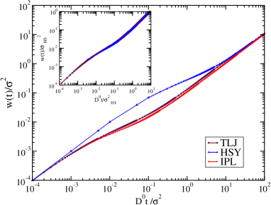
Figure 7: BD results for the MSD of the systems in Fig. 3, in original units (main panel), and scaled with the hard-sphere unit.

In the long-time regime, on the other hand, the MSD reads $[W(t)/\sigma^{2}]\approx D^{*}[D^{0}t/\sigma^{2}]$, i.e., it is proportional to the scaled long-time self-diffusion coefficient $D^{*}$, defined as

$$D^{*}\equiv D_{L}/D^{0}.$$ (29)

This property does depend on the interparticle interactions, and hence, on the particular system and on its state, i.e., $D^{*}=D^{*}(T^{*},\phi,\nu)$. Thus, the various $W(t)$ in Fig. 7 should differ in their long-time behavior. They, however, exhibit the same long-time limit. The reason for this is that the dynamic equivalence condition in Eq. (25) implies that the dimensionless parameter $D^{*}$ depends on $(T^{*},\phi,\nu)$ only through the effective HS volume fraction $\phi_{HS}=\phi_{HS}(T^{*},\phi,\nu)$,

$$D^{*}(T^{*},\phi,\nu)\approx D^{*}_{HS}[\phi_{HS}(T^{*},\phi,\nu)],$$ (30)

and the three systems in Fig. 3 were chosen to have the same $\phi_{HS}\ (=0.49)$. Thus, they share the same value of $D^{*}(\approx 0.1)$.

In fact, for the very same reason (see the scaling in Eq. (28)) these three systems must actually share the full dependence of $W^{*}(t^{*})$ on the scaled time $t^{*}\equiv D^{0}t/\sigma_{HS}^{2}$, i.e., the three different MSDs in Fig. 7 should collapse onto the same curve when plotted as a function of $t^{*}$. This is indeed what we find, as illustrated in the inset of this figure. Furthermore, according to Eq. (28), the resulting master curve then determines the function $W^{*}_{HS}[t^{*};\phi=0.49]$. The SCGLE theory for Brownian systems (i.e., Eqs. (21)-(24)), besides predicting this scaling also provides an approximate prediction for this function. The results of the SCGLE theory applied to the HS fluid follow closely the simulations results.

The results presented in this figure are concerned with the full MSD of three model systems that share the same effective volume fraction $\phi_{HS}=0.49$. Let us next extend our study to a wider range of effective HS volume fractions, focusing on long-time properties such as the long-time self-diffusion coefficient $D_{L}$ and the $\alpha$-relaxation time $\tau_{\alpha}$. We start by presenting in Fig. 8(a) the BD results for the inverse of $D^{*}=D_{L}/D^{0}$ as a function of the respective volume fraction $\phi$ for several soft-sphere systems. The main panel of the figure shows how the simulated $D^{*}$ of three TLJ systems depends on volume fraction and on softness. For instance, $D^{*}$ is, as expected, a decreasing function of $\phi$ and $\nu$, and in the low-$\phi$ limit all the results converge to the correct limiting value $D^{*}(\phi\to 0)=1$. For reference, in this figure we include the approximate SCGLE prediction of the function $D^{*}_{HS}(\phi)$ corresponding to the HS fluid (the solid line in the figure). It is clear that as the potential becomes stiffer the function $D^{*}(\phi)$ gradually approaches the function $D^{*}_{HS}(\phi)$.

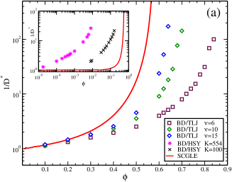
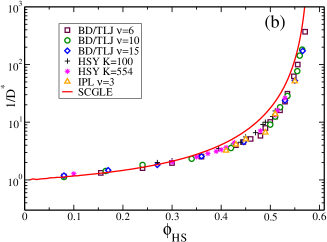
Figure 8: Inset (a): $D^{*}=D_{L}/D^{0}$ from DB simulations for TLJ systems with $\nu=6$, $\nu=10$ and $\nu=15$, at different volume fractions $\phi$. Inset: Results for two HSY systems ($K=554$, $z=0.149$, and $K=100$ $z=1.0$). Inset (b): Results plotted as a function of $\phi_{HS}$.Data for the IPL($\nu=3$) is included. The solid line represents the solution for HS systems from the colloidal SCGLE theory.

Model systems with longer-ranged interactions can depart even further from this HS limit. Thus, in the inset of the same figure we compare the results for $D^{*}(\phi)$ of two HSY systems with the predicted HS limit (also represented by the solid line). This comparison exhibits a much more pronounced difference compared with the shorter-ranged systems in the main panel. Here the values of $D^{*}$ in the liquid regime of the HSY systems correspond to volume fractions in the range $10^{-5}-10^{-1}$ (from weakly to highly structured conditions), whereas the relevant volume fractions of the TLJ systems fall in the typical range $0.1\lesssim\phi\lesssim 1$. Despite these differences, however, when these data, as well as the data for the TLJ systems in the main figure, are plotted as suggested by the scaling in Eq. (30), all of them fall on a well-defined master curve, as demonstrated in Fig. 8(b). This master curve must then determine the exact hard-sphere function $D^{*}_{HS}[\phi]$. The solid line in the figure is the corresponding approximate SCGLE prediction for this function, whose comparison with the exact master curve defined by the collapsed simulation data indicates the level of quantitative accuracy of this theory.

Let us notice that, although the results in the figure illustrate the dynamic equivalence at the very particular condition $t\rightarrow\infty$, our simulations show that basically the same scaling holds at all times for time-dependent properties such as the scaled time-dependent self-diffusion coefficient $D^{*}(t)\equiv W(t)/6D^{0}t$ (illustrated in Fig. 4 of Ref. dynamicequivalence )), or the scaled MSD $W^{*}(t^{*})$, illustrated here in Fig. 7 with the results of three model systems that meet the condition $\lambda_{n}\approx 1$ at an effective volume fraction is $\phi_{HS}=0.49$. We have extended this study, however, to the IPL and HSY potentials at low effective HS volume fractions, the regime in which appreciable deviations from the condition $\lambda_{n}$ are exhibited (see Fig. 4). The corresponding scaled results for $D^{*}(\phi_{HS})$, presented in Fig. 8(b), demonstrate that the predicted dynamic equivalence has a wide range of validity, requiring only the static structural equivalence discussed in Sec. III, but not necessarily the condition $n_{HS}\approx n$, in spite of the fact that our original insight of the soft-hard dynamic equivalence derived from the structure of the SCGLE equations within the condition $\lambda_{n}=n_{HS}/n\approx 1$.

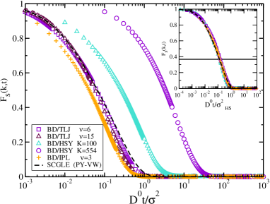
Figure 9: $F_{S}(k_{max},t)$ from BD simulations for two TLJ systems with $\nu=6$ and $\nu=15$, IPL system, and two Yukawa systems . All systems have an effective volume fraction $\phi_{HS}=0.49$. In the inset the results are presented as a function of $D^{0}t/\sigma_{HS}^{2}$ and $k\sigma_{HS}$, with $k=k_{max}$.

Let us now turn our attention to the relaxation of the intermediate scattering function $F_{S}(k,t)$. To exhibit the dynamic equivalence predicted by Eq. (25), we evaluate $F_{S}(k,t)$ for two TLJ and two HSY systems at states that share the same equivalent volume fraction, $\phi_{HS}=0.49$. In the main frame of Fig. 9 we plot $F_{S}(k_{max},t)$ as a function of the scaled time $D^{0}t/\sigma^{2}$, a format in which the results for the TLJ and HSY systems differ notoriously. In particular, the $\alpha$-relaxation time $\tau_{\alpha}$ of these systems, defined by the condition $F_{S}(k,\tau_{\alpha})=1/e$, differ by more than one decade. According to Eq. (25), however, the same results should collapse onto a single master curve upon the transformation to HS units, and provided that $F_{S}(k,t)$ for the various systems is evaluated at structurally equivalent wave-vectors (i.e., same value of $k\sigma_{HS}$). To meet this iso-structural requirement for the three systems in the figure we have evaluated $F_{S}(k,t)$ at the position $k_{max}$ of the corresponding static structure factors. The resulting master curve is shown in the inset of the figure, in which the data are plotted as a function of the scaled time $D^{0}t/\sigma_{HS}^{2}$. Such scaling of $F_{S}(k,t)$, in its turn, leads to identical $\alpha$-relaxation times for iso-structural systems, when expressed in the new units, regardless of the softness or range of the interaction between the particles.

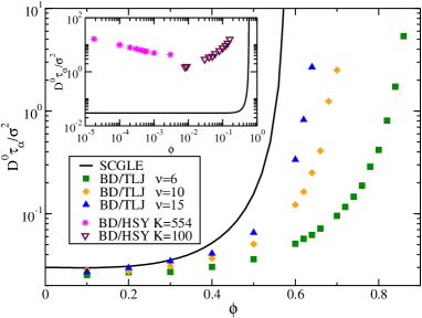
Figure 10: $\tau_{\alpha}(\phi)$, in BD units, for TLJ systems. The solid line represents the SCGLE results for HS systems. Inset: Results for two HSY systems.

Another manner to exhibit this dynamic equivalence starts with the BD simulations of the $\alpha$-relaxation time, for several soft-sphere systems in an extended range of volume fractions, evaluated at a structurally identical wave-vector (we take $k=k_{max}$). In the main panel of Fig. 10 we present the unscaled results for $\tau_{\alpha}$ corresponding to the TLJ systems with $\nu=6$, $\nu=10$ and $\nu=15$. There we observe that $\tau_{\alpha}$ exhibits the typical monotonic slowing down with concentration, increasing faster at higher $\phi$, at a rate that depends strongly on the softness of the potential, following a similar pattern as $1/D^{*}$ in the mainframe of Fig. 8(a). Here too, increasing $\nu$ leads to results progressively closer to the curve predicted by the SCGLE theory for the HS system, represented in the figure by the solid line.

In contrast, the corresponding simulation data of $\tau_{\alpha}$ for the longer-ranged HSY systems, presented in the inset of Fig. 10, exhibit a notoriously different $\phi$-dependence. The difference is mainly quantitative in the case of the HSY system with $K=100$ and $z=1.0$, since the results for $\tau_{\alpha}$ presented in the figure also increase monotonically, although at much smaller values of $\phi$ with respect to the hard-sphere system (represented again by the solid line). In the case of the system with $K=554$ and $z=0.149$, however, the corresponding differences seem to be even qualitative, since the data presented change non-monotonically with $\phi$. Although this contrast may appear dramatic, however, it actually reflects a rather trivial consequence of the facts that at low volume fractions $\tau_{\alpha}\approx 1/k^{2}D^{0}$ and that for this long-ranged, strongly-interacting, HSY system, $k_{max}\approx 2\pi/n^{-1/3}$; thus, at low volume fractions $\tau_{\alpha}\propto\phi^{-2/3}$. Thus, this qualitative feature would be absent if we had plotted $\tau^{*}\equiv k^{2}D^{0}\tau_{\alpha}$, rather than the unscaled $\alpha$-relaxation time.

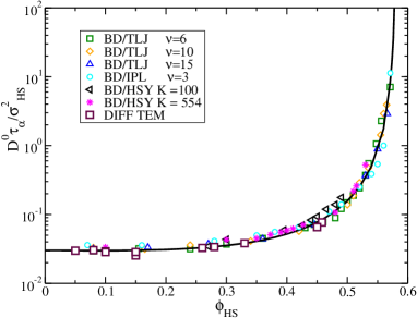
Figure 11: $\alpha$-relaxation time $\tau_{\alpha}$, in HS units, as a function of $\phi_{HS}$. The solid line corresponds to the results from the SCGLE theory applied to HS fluids.

This scaling, however, will only remove the apparently anomalous $\phi$-dependence of $\tau_{\alpha}$, but not the quantitative difference in the range of volume fractions at which the sharp increase of $\tau_{\alpha}$ occurs. However, the dynamic scaling in Eq. (25), illustrated in Fig. 9 with $F_{S}(k,t)$ for the case $\phi_{HS}=0.49$, should now align the data for $\tau_{\alpha}(\phi)$ in Fig. 10 with those of the HS system upon the transformation to HS units. For this we mean to plot $\tau_{\alpha}$ scaled as $D^{0}\tau_{\alpha}/\sigma_{HS}^{2}$, as a function of $\phi_{HS}(\phi,T^{*})$. This is done in Fig. 11, where we corroborate that indeed the transformed data fall in a master curve that follows closely the solid line, i.e., the SCGLE theoretical predictions for the HS fluid.

IV.2 Atomic liquids

Let us now discuss this dynamic equivalence in the context of atomic liquids. For this, let us notice that in order to discus the dynamic equivalence between soft- and hard-sphere Brownian fluids we first unambiguously defined an effective hard-sphere volume fraction and diameter, $\phi_{HS}=\phi_{HS}(\phi,T^{*})$ and $\sigma_{HS}=\sigma_{HS}(\phi,T^{*})$, for each state $(\phi,T^{*})$ of the soft-sphere system. Then, the dynamic equivalence was simply exhibited by expressing the dimensionless properties of the system not in terms of the natural units of the soft system, namely, $\phi$, $\sigma$, and $t^{0}\equiv\sigma^{2}/D^{0}$, but in terms of the units of the equivalent HS system, namely, $\phi_{HS}$, $\sigma_{HS}$, and $t^{0}_{HS}\equiv\sigma^{2}_{HS}/D^{0}=\lambda^{2}_{\sigma}t^{0}$. Since the definition of the effective hard-sphere diameter only involves the comparison of the equilibrium static structure of the soft-sphere system with the corresponding structure of the equivalent hard-sphere system (see Eq. (13)), it is natural to expect that the dynamic equivalence discussed above in the context of Brownian systems also holds independently of the underlying microscopic dynamics, i.e., also for atomic liquids.

Thus, let us now discuss the dynamic equivalence between atomic soft-sphere systems and their effective atomic hard-sphere counterpart. For this, let us follow the same principle as in the Brownian case, i.e., let us express the dynamic properties of Newtonian liquids not in terms of their “natural” units $\phi$, $\sigma$, and $t^{0}=\sigma/v_{0}=\sqrt{M\sigma^{2}/k_{B}T}$, but in terms of the units of the equivalent HS system, namely, $\phi_{HS}$, $\sigma_{HS}$, and $t^{0}_{HS}\equiv\sqrt{M\sigma^{2}_{HS}/k_{B}T}=\lambda_{\sigma}t^{0}$. To see the accuracy of this predicted scaling of atomic fluids, in Fig. 12 we present the MD simulation results for the MSD of some of the illustrative model systems employed before, namely, the TLJ system with $\nu=6$ and $10$, a HSY system with $K=554$ and $z=0.149$, all of them at the effective volume fraction $\phi_{HS}=0.49$. At the same time, we include the corresponding data for the hard spheres fluid, obtained from event-driven MD simulations as described in gabriel . In the main frame of Fig. 12 the MSD is scaled in the usual MD units, i.e., as $W(t)/\sigma^{2}$, plotted vs. the time scaled as $t/t^{0}$.

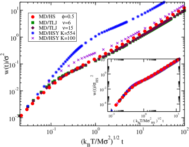
Figure 12: MSD from MD simulations for iso-structural soft systems with equivalent $\phi_{HS}=0.49$. The filled circles correspond to the MD simulations of a HS fluid. The results are presented in units of $\sigma$ and $t^{0}$. Inset: MSDs after transforming to HS units.

As observed in the figure, the results for the various systems clearly display the ballistic ($W(t)\sim v_{0}^{2}t^{2}$) and diffusive ($W(t)\sim D_{L}t$) regimes characteristic of the underlying Newtonian dynamics. They also exhibit their departure from the exact HS results, particularly noticeable in the HSY system. In HS units, on the other hand, the different curves in the main panel of the figure should fall on top of the HS data, and this is verified in the inset of the figure, which shows the MSD scaled as $W(t)/\sigma^{2}_{HS}\ [=\lambda^{-2}_{\sigma}W(t)/\sigma^{2}]$, plotted vs. the scaled time as $t/t^{0}=\ [\lambda^{-1}_{\sigma}t/t^{0}]$. By scaling in this manner we appreciate that all the soft, iso-structural systems follow basically the same time evolution, sharing, in particular, a common scaled long-time self-diffusion coefficient.

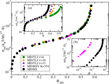
Figure 13: Inset (a): $D_{L}(\phi)$ scaled with $\sigma^{2}/t^{0}=\sigma\sqrt{k_{B}T/M}$ fot TLJ systems. Inset (b): Results for HSY systems. Main Panel: Results in the insets after transform to HS units. The results for strictly HS system are represented by the filled circles correspond to HS systems.

From the long-time limit of the results in the mainframe of Fig. 12, one can read the value of the long-time self-diffusion coefficient $D_{L}$ in units of $\sigma^{2}/t^{0}=\sigma\sqrt{k_{B}T/M}$. We have collected these values of $D_{L}$ for each of the systems considered here as a function of the volume fraction $\phi$ of the systems, and the results are summarized in the two insets of Fig. 13. The inset 13 (a) contains the results for the TLJ systems, whereas the inset 13 (b) illustrates the noticeable contrast between the HS and the strongly repulsive HSY system. At intermediate and high volume fractions these data exhibit similar trends to those observed in the corresponding BD simulations (in Fig. 8(a)). The main qualitative difference between atomic and Brownian systems can be observed at low volume fractions, where, in contrast to Brownian systems,the atomic $D_{L}$ behaves as $D_{L}\sim 1/\phi$ , at low volume fraction as the expected from the kinetic theory of dilute gases mcquarrie .

If, on the other hand, the soft-hard dynamic equivalence were to apply to these atomic systems, all of the data of $D_{L}$ displayed in these two insets should collapse on a master curve when $D_{L}$ is expressed not in its ordinary atomic units, but in the corresponding HS units, $\sigma_{HS}/t^{0}_{HS}=\sigma_{HS}\sqrt{k_{B}T/M}$, and plotted not as a function of $\phi$, but of the effective HS volume fraction $\phi_{HS}(T^{*},\phi)$. The mainframe of Fig. 13 plots the data in the inset in precisely this manner. From these results we see clearly that the soft systems follow very well the corresponding data for truly hard spheres in all the range of volume fractions considered in the figure, thus corroborating the expected validity of the dynamic equivalence between soft- and hard-sphere atomic liquids.

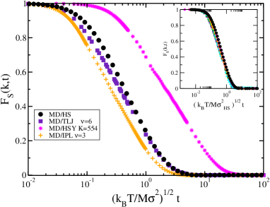
Figure 14: $F_{S}(k,t)$ from MD simulations for TLJ ($\nu=6,15$), IPL ($\nu=3$), and HSY ($K=554$) systems with equivalent volume fraction $\phi_{HS}=0.49$. Time is in units of $t^{0}=\sqrt{\sigma^{2}M/k_{B}T}$. Inset: Results after transforming to HS units via $t_{HS}=\lambda_{\sigma}t^{0}$. $k=k_{max}$ is used.

To close this section let us focus on the scaling properties of the atomic self-ISF and its characteristic $\alpha$-relaxation time. Thus, in figure (14) we present $F_{S}(k_{max},t)$ for the TLJ ($\nu=6$), IPL ($\nu=3$), HSY ($K=554$), and HS systems, all of them with equivalent HS volume fraction $\phi_{HS}=0.49$. In the main panel, where the time is expressed in its natural atomic units, one can see the contrast between the various soft and the HS systems, with a scenario rather similar to that found for Brownian fluids. In the inset, on the other hand, we replot the same data but now as a function of the time expressed in the HS time units $\sqrt{M\sigma^{2}_{HS}/k_{B}T}$. There one can appreciate the sustancial agreement between the different iso-structural systems, which closely follow the same time-evolution in this scaled form, with virtually the same scaled $\alpha$-relaxation time $(k_{B}T/M\sigma^{2}_{HS})^{1/2}\tau_{\alpha}$.

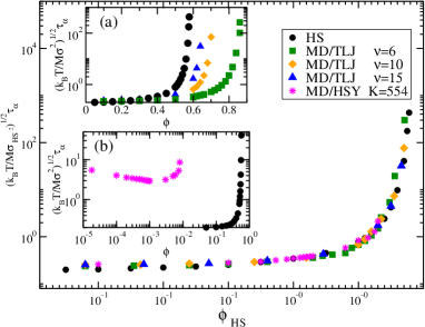
Figure 15: $\tau_{\alpha}(\phi)$, for selected TLJ, IPL, and HSY systems. In the three panels, the filled circles correspond to the results for HS systems. Inset (a): $\tau_{\alpha}(\phi)$, in MD units, for TLJ systems with $\nu=6,10,15$. Inset (b): $\tau_{\alpha}(\phi)$, in MD units, for HSY systems with $K=554$ and $z=0.149$. Main panel: Collection of results for $\tau_{\alpha}(\phi)$ in HS units.

In Fig. 15 we present data of $\tau_{\alpha}$ obtained from similar simulations of $F_{S}(k_{max},t)$ for the various systems carried out varying the density. These data are plotted as a function of the respective volume fraction $\phi$ in the ordinary atomic units (insets), and normalized with the HS units (main panel). In general, again, the trends here resemble closely those of the Brownian systems previously discussed, in the sense that the completely disperse unscaled data in the insets, in the main panel, collapse nicely onto a master curve that coincides, of course, with the MD data of strictly hard spheres (black symbols). This concludes the present discussion of the soft-hard dynamic equivalence in both, atomic and Brownian liquids. In what follows we discuss a related but fundamentally different scaling.

V Brownian-Atomic Dynamic Equivalence

As mentioned in the introduction, the second fundamental challenge in understanding the relationship between dynamic arrest phenomena in colloidal systems and the glass transition in atomic liquids is to determine the role played by the underlying (Brownian vs. Newtonian) microscopic dynamics. The results presented in the previous section provide one step forward in this direction, since they demonstrate that the criterion to unify a rather diverse set of soft-sphere systems in a so-called dynamic universality class is actually independent of the Brownian or Newtonian nature of their microscopic dynamics. As a result, for example, the data for the long-time self-diffusion coefficient $D_{L}$ of various Brownian systems, displayed in Fig. 8(a), collapse onto the master curve of Fig. 8(b). In its turn, the data for $D_{L}$ of the atomic version of the same systems, shown in the insets of Fig. 13, collapse onto their own master curve, displayed in the main frame of the same figure.

An important question, however, is left open by these results. It refers to the possibility that a fundamental relationship can be established, now between those two master curves (in Figs. 8(b) and 13 respectively), which would unify the dynamics of an atomic liquid with the dynamics of its Brownian counterpart in an unambiguous and precise manner. This question was largely answered theoretically in recent attempts of our group to extend the SCGLE theory of colloid dynamics to atomic systems atomic1 ; atomic2 . There it was established that such a relationship is provided by the recognition that the (density- and temperature-dependent) self-diffusion coefficient of an atomic liquid, determined by kinetic theoretical arguments as

$$D^{0}=\frac{3}{8\sqrt{\pi}}\left(\frac{k_{B}T}{M}\right)^{1/2}\left(\frac{1}{n\sigma_{HS}^{2}}\right),$$ (31)

plays the role of the short-time self-diffusion coefficient $D^{0}$ in Brownian systems.

As a result, in Refs. atomic1 ; atomic2 it was predicted, for example, that the ratio $D^{*}\equiv D_{L}/D^{0}$ of the long-time to the short-time self-diffusion coefficients of a Brownian system must be identical to the long-time self-diffusion coefficient of the corresponding atomic liquid, scaled with this kinetic theoretical value of $D^{0}$. Testing this particular prediction is, of course, very straightforward, and can be done by normalizing the data of $D_{L}$ for the atomic systems in the insets of Fig. 13, with the value of $D_{0}$ given by Eq. (31). The resulting scaled data should then coincide with the corresponding results for $D^{*}$ of the Brownian version of the same systems in Fig. 8(a).

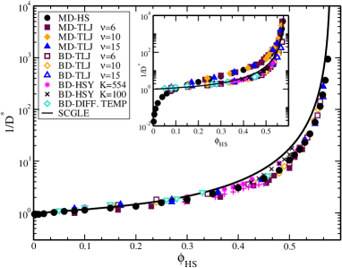
Figure 16: Scaled results for the long time diffusion coefficient for colloid and atomic liquids. In the main panel $D^{*}(\phi_{HS})=D_{L}/D^{0}$ is plotted using the corresponding definition of $D^{0}$. Inset: $D_{L}(\phi_{HS})$ in HS units as reported in the previous Figs. 8(b) and 13.

The same comparison, however, can be done more directly if we take the same data, but after they have been collapsed onto their respective master curve in Figs. 8(b) and 13. Thus, in the inset of Fig. 16 we reproduce these two master curves, to highlight the different behavior of atomic and Brownian liquids regarding the density dependence of the data for $D_{L}$ expressed in the effective HS units. The next step is then to scale the atomic data for $D_{L}$ as $D^{*}\equiv D_{L}/D^{0}$ with $D_{0}$ given by Eq. (31). The result of this scaling is that the original atomic master curve now coincides with the original Brownian master curve, as demonstrated in the main frame of Fig. 16. Since the Brownian data for $D_{L}$ were already expressed as $D^{*}\equiv D_{L}/D^{0}$, this collapse between both master curves illustrates the accuracy of the predicted dynamic equivalence between atomic and Brownian liquids.

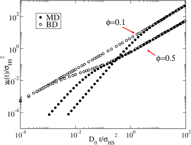
Figure 17: Mean squared displacement, from molecular dynamics (solid symbols) and Brownian dynamics ( empty symbols)simulation, for equivalent hard-sphere systems, for states corresponding to $\phi_{HS}=0.1$ and $0.5$.

As originally proposed, however, the atomic-Brownian scaling extends to the time-dependent dynamic properties, such as the mean squared displacement and the self intermediate scattering functions. Thus, in Refs. atomic1 ; atomic2 it was predicted that these properties of a given atomic liquid, at times $t$ much longer than the mean free time, and with $t$ scaled with $D^{0}$ in Eq. (31), will be indistinguishable from those of its Brownian counterpart. To illustrate such condition, the atomic and Brownian MSD of the TLJ potential with $\nu=6$ and effective HS volume fractions $\phi_{HS}=0.1$ and $0.5$, are presented in Fig. 17 in the format $W(t)/\sigma^{2}_{HS}$ vs. $D_{0}t/\sigma_{HS}^{2}$ (i.e. in HS units). The results clearly show that despite the differences at short times (ballistic vs. diffusive), the MSDs of iso-structural systems do collapse onto each other in the long-time regime.

This long-time atomic-Brownian scaling can also be observed in $F_{S}(k,t)$. However, in contrast with the MSD, in which this scaling holds at all effective volume fractions, in the case of $F_{S}(k,t)$ this scaling only holds above a certain threshold effective volume fractions, corresponding essentially to the metastable liquid regime. This is illustrated in Fig. 18, where we present molecular and Brownian dynamics results for this property at three volume fractions of the effective hard-sphere liquid, $\phi_{HS}=0.50,0.548$, and $0.571$ (generated, in reality, with the dynamically equivalent TLJ potential with $\nu=6$). In this figure $F_{S}(k,t)$ is plotted as a function of the dimensionless time $D^{0}t/\sigma^{2}_{HS}$, with the corresponding $D^{0}$ for each dynamics (i.e., given by Eq. (31) in the atomic version of the system).

As indicated above, this long-time dynamic equivalence between atomic and Brownian liquids is not observed in $F_{S}(k,t)$ at low volume fractions corresponding to the stable fluid regime (i.e., for $\phi_{HS}\lesssim 0.5$). This is illustrated in Fig. 18 with the atomic and Brownian results for $F_{S}(k,t)$ corresponding to $\phi_{HS}=0.1$, which totally fail to collapse on top of each other, especially at long times. The reason for this deviation from the long-time dynamic equivalence at low volume fractions is that in this regime, the decay of the atomic $F_{S}(k,t)$ to a value $\approx e^{-1}$ occurs within times comparable to the mean free time $\tau_{0}$ and is, hence, intrinsically ballistic. It is only at higher volume fractions that this long-time dynamic equivalence is fully exhibited by the diffusive decay of $F_{S}(k,t)$, as illustrated by the three largest volume fractions in the figure.

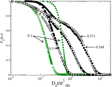
Figure 18: MD (solid symbols) and BD (empty symbols) simulation results for the $F_{S}(k,t)$ of equivalent HS liquids at volume fractions $\phi_{HS}=0.10,0.50,0.548$ and $0.571$, evaluated at the main peak of the static structure factor and plotted as a function of the dimensionless time $D^{0}t/\sigma^{2}_{HS}$.

The observations above can also be summarized by comparing the volume fraction dependence of the relaxation time $\tau_{\alpha}$ of the molecular and Brownian versions of the various soft-sphere systems discussed in the previous section. Such results were summarized in the Brownian and atomic master curves presented, respectively, in Figs. (11) and (15), which we now put together in the inset of Fig. 19. To exhibit the long-time dynamic equivalence between atomic and Brownian fluids, the same results are presented again in the main panel of the figure, but now scaled as $\tau^{*}\equiv k^{2}D^{0}\tau_{\alpha}$ with $k=k_{max}$ in HS units. From the corresponding comparison one can see that this long-time dynamic equivalence, which manifests itself in the collapse of the molecular and Brownian dynamics data for $\tau^{*}$, holds only above a threshold volume fraction, roughly located near the freezing transition of the HS liquid ($\phi_{HS}\approx 0.5$). The qualitative difference between atomic and Brownian systems observed in the results for $\tau^{*}$ for volume fractions below this threshold are explained in the different low-density limit of $\tau^{*}$ in each case. For a Brownian liquid $\tau_{\alpha}\rightarrow 1/k^{2}D^{0}$ as $\phi\rightarrow 0$, with a $\phi$-independent short-time diffusion coefficient $D^{0}$, so that $\tau^{*}\rightarrow 1$ as $\phi\rightarrow 0$. For atomic liquids, however, $\tau^{*}\rightarrow\sqrt{2\pi}k\sigma/16\phi$ in the same limit, where we have taken into account the fact that in this case the short-time diffusion coefficient $D^{0}$ is given by the kinetic-theoretical result in equation (31).

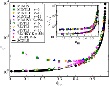
Figure 19: Inset: $\alpha$-relaxation time $\tau_{\alpha}(\phi_{HS})$ for Brownian and Molecular liquids in HS units as reported in the previous Figs. 11 and 15. Main panel: Data presented as $\tau^{*}\equiv k^{2}D_{0}\tau_{\alpha}$. The solid curve is the prediction for $\tau^{*}$ for the colloidal SCGLE.

VI Summary

In this work we have presented an extended simulation study on the static and dynamic equivalence between model fluids with soft repulsive potentials of varying range and strength, governed by either Brownian or atomic microscopic dynamics. The dynamic equivalence investigated here relies heavily on the concept of static structural equivalence proposed by Weeks, Chandler and Andersen, i.e., on the notion that the thermodynamic and structural properties of fluids formed by moderately soft particles can be expressed in terms of the properties of the hard-sphere liquid.

Thus, the present work started by reviewing such concept of structural mapping, explaining how this idea is extended to map the static structure of, in principle, any soft-sphere liquid onto the properties of an effective hard-sphere liquid. We provided details of the method adopted to identify structurally equivalent systems, which works better than other traditional approaches, such as the blip function method, especially for long-ranged potentials. We also explained how to extend this mapping procedure to the case of polydisperse systems, which allowed us to study highly concentrated systems beyond freezing, i.e., in the metastable liquid fase.

This structural equivalence was then employed in the study of the dynamic equivalence between iso-structural colloidal fluids. For this, simple rules are provided to map the units of length and time for soft systems to those of the equivalent HS systems. Our extensive Brownian dynamics simulations verified, for example, that the mean square displacement and the self intermediate scattering functions of iso-structural systems follow the same time evolution when they are expressed in the units of the equivalent HS system. In particular, data were provided as a function of the volume fraction, covering from dilute to highly concentrated conditions, to show that long time properties such as the long time self diffusion coefficient and the $\alpha$-relaxation time of soft colloidal systems collapse onto a master curve when plotted as a function of the (density- and temperature-dependent) effective HS volume fraction. Furthermore, we showed that this dynamic equivalence extends over to the domain of atomic fluids. Thus, in Sect. IV we demonstrated that the criterion that unifies the soft-sphere systems in the hard-sphere dynamic universality class is actually independent of the Brownian or Newtonian nature of their microscopic dynamics, in the sense that the properties of Brownian systems collapse onto a given master curve, as in Fig. 8(b), and the same applies to the atomic version of the same systems, whose properties collapse onto their own master curve, as in Fig. 13.

The findings just described then reveal that the dynamics of soft systems can be mapped onto those of HS systems, regardless of the underlying Brownian or Newtonian dynamics, i.e., both type of systems satisfy a soft-hard dynamics equivalence. Going further, however, the inspection of the long-time behavior of atomic liquids revealed another connection, this time between colloidal and atomic fluids. This connection was established once the atomic-liquid analog of the Brownian short-time self-diffusion coefficient $D^{0}$ is identified with the the value predicted by the kinetic theory of gases, i.e., by $D^{0}$ given in Eq. (31). The simulation evidence that we provide here corroborate that at least for model liquids whose structure is dominated by (soft- or hard-sphere) repulsive interactions, the long-time dynamics of an atomic liquid is indistinguishable from the dynamics of the colloidal system with the same inter-particle interactions. As a consequence, some dimensionless long-time dynamic properties, such as $D^{*}=D_{L}/D^{0}$ (with the proper identification of $D^{0}$) and $\tau^{*}(k)=k^{2}D^{0}\tau_{\alpha}$ (only in the supercooled liquid regime) will exhibit, just like the equilibrium thermodynamic and structural properties, the same independence from the short-time microscopic dynamics, which otherwise distinguishes atomic from colloidal systems.

Let us clarify that for the present study we chose to focus on a well-defined set of model systems, namely, systems with purely repulsive soft-sphere interactions of arbitrary range. This excludes from this study the consideration, for example, of the possibility of full overlap between particles, characteristic of ultrasoft interactions likos . Hence, a pending question is the degree at which the scalings discussed in this work will apply to these systems. Similarly, the absence of attractive forces in our working examples leaves open the issue of the possible extension of these scalings to systems that involve attractive interparticle forces. We have performed, however, preliminary calculations with both, ultrasoft systems and systems with attractive interactions, and the results suggest that these scalings have a much wider range of applicability. Another important aspect that requires further discussion is the relationship of the dynamic scalings discussed in this work and other scalings discussed in the literature. We have mostly in mind the interesting concept of strongly correlated liquids, developed by J. Dyre and collaborators dyrejpcm2013 ; gnan1 ; gnan2 ; dyreprx . It will be interesting to clarify, for example, if the concept of isomorphic states defined from their perspective, is related to our findings that isostructurality is also associated with isodiffusivity.

On the other hand, and as a final remark, let us mention that here we referred to Brownian liquids as colloidal suspensions, with the intention to connect with real physical systems. In reality, however, we really meant colloidal systems for which hydrodynamic interactions can be neglected, since these important effects were completely ignored in our Brownian dynamics simulations. We expect, however, that most of our conclusions will apply to real colloidal systems in which hydrodynamic interactions are important, as long as we identify the parameter $D^{0}$ not with the value of the long-time self-diffusion coefficient $D_{L}$ at infinite dilution ($\phi=0$), but with the $\phi$-dependent short-time self-diffusion coefficient $D_{S}(\phi)$ prlhi , which under some circumstances can be independently determined either theoretical or experimental methods. Fig. 3 of Ref. gabriel illustrates the effectiveness of this hydrodynamic scaling, which is expected to expand the range of application of the soft-to-hard and Brownian-to-atomic dynamic equivalences discussed in this work.

ACKNOWLEDGMENTS: This work was supported by the Consejo Nacional de Ciencia y Tecnología (CONACYT, México), through grants No. 132540 and 182132.

References

- (1) Angell C. A., Ngai K. L., McKenna G. B., McMillan P. F. and Martin S. F., J. Appl. Phys. 88 3113 (2000).
- (2) M. D. Ediger, C. A. Angell, and S. R. Nagel, J. Phys. Chem.100, 13200 (1996)
- (3) K. L. Ngai, D. Prevosto, S. Capaccioli and C. M. Roland, J. Phys.: Condens. Matter 20, 244125 (2008)
- (4) C. A. Angell, Science 267, 1924 (1995).
- (5) P. G. Debenedetti and F. H. Stillinger, Nature 410, 359 (2001).
- (6) F. Sciortino and P. Tartaglia, Adv. Phys. 54, 471 (2005).
- (7) Jamming and Rheology: Constrained Dynamics on Microscopic and Macroscopic Scales, edited by A. J. Liu and S. R. Nagel (Taylor & Francis, New York, 2001).
- (8) N. Xu, T. K. Haxton, A. J. Liu, and S. R. Nagel, Phys. Rev. Lett. 103 245701 (2009).
- (9) L. Berthier and T. A. Witten, Europhys. Lett. 86, 10001 (2009).
- (10) H. Löwen, J. P. Hansen, and J. N. Roux, Phys. Rev. A 44, 1169 (1991).
- (11) G. Szamel and E. Flenner, Europhys. Lett., 67, 779 (2004).
- (12) A. M. Puertas, J. Phys.: Condens. Matter 22, 104121 (2010).
- (13) W. Götze, in Liquids, Freezing and Glass Transition, edited by J. P. Hansen, D. Levesque, and J. Zinn-Justin (North-Holland, Amsterdam, 1991).
- (14) G. Szamel and H. Löwen, Phys. Rev. A 44, 8215 (1991).
- (15) L. Bøhling et al., J. Phys.: Condens. Matter, 25, 032101 (2013).
- (16) J. L. Boon and S. Yip, Molecular Hydrodynamics (Dover Publications Inc. N. Y., 1980).
- (17) M. Medina-Noyola, Faraday Discuss. Chem. Soc. 83, 21 (1987).
- (18) M. Medina-Noyola and J. L. del Río-Correa, Physica 146A, 483 (1987).
- (19) L. Yeomans-Reyna and M. Medina-Noyola, Phys. Rev. E 62, 3382 (2000).
- (20) L. Yeomans-Reyna and M. Medina-Noyola, Phys. Rev. E 64, 066114 (2001).
- (21) L. Yeomans-Reyna, H. Acuña-Campa, F. Guevara-Rodríguez, and M. Medina-Noyola, Phys. Rev. E 67, 021108 (2003).
- (22) P.E. Ramírez-González et al., Rev. Mex. Física 53, 327 (2007).
- (23) L. Yeomans-Reyna et al., Phys. Rev. E 76, 041504 (2007).
- (24) R. Juárez-Maldonado et al., Phys. Rev. E 76, 062502 (2007).
- (25) P. E. Ramírez-González and M. Medina-Noyola, Phys. Rev. E 82, 061503 (2010); ibid. Phys. Rev. E 82, 061504 (2010).
- (26) P. E. Ramírez-González and M. Medina-Noyola, Phys. Rev. E 82, 061503 (2010); ibid. Phys. Rev. E 82, 061504 (2010).
- (27) P. E. Ramírez-González and M. Medina-Noyola, J. Phys.: Cond. Matter, 21, 75101 (2009).
- (28) P. E. Ramírez-González, L. López-Flores, H. Acuña-Campa, and M. Medina-Noyola, Phys. Rev. Lett. 107, 155701 (2011).
- (29) H. C.Andersen, J. D. Weeks and D. Chandler, Phys. Rev. A 4, 1597 (1971).
- (30) J.P. Hansen and I.R. McDonald, Theory of Simple Liquids (Academic Press Inc., 1976)
- (31) P. Mendoza-Méndez, L. López-Flores, A. Vizcarra-Rendón, L. E. Sánchez-Díaz, and M. Medina-Noyola, arXiv:1203.3893v1 [cond-mat.soft].
- (32) L. López-Flores, L. L. Yeomans-Reyna, M. Chávez-Páez, and M. Medina-Noyola, J. Phys.: Condens. Matter, 24 375107 (2012).
- (33) G. Nägele, Phys. Rep. 272, 215 (1996).
- (34) K.J. Gaylor, I.K. Snook, W. van Megen, and R.O. Watts, J. Phys. A 13, 2513 (1980).
- (35) M.P. Allen and D.J. Tildesley, Computer Simulation of Liquids, (Oxford, University Press, 1887.)
- (36) T.S. Grigera and G. Parisi, Phys. Rev. E 63, 45102(R), (2001).
- (37) D. Dubbeldam, D.C. Ford, D.E. Ellis, and R.Q. Snurr, Mol. Phys. 35, 1084 (2009).
- (38) J.S. van Duijneveldt and D. Frenkel, J. Chem. Phys. 96, 4655 (1992).
- (39) G. Pérez-Ángel et al., Phys. Rev. E 83, 060501 (2011).
- (40) J. K. Percus and G. J. Yevick, Phys. Rev. 110, 1 (1957).
- (41) M. S. Wertheim, Phys. Rev. Lett. 10, 321 (1963).
- (42) L. Verlet and J.-J. Weis, Phys. Rev. A 5 939 (1972).
- (43) F. de J. Guevara-Rodríguez and M. Medina-Noyola, Phys. Rev. E 68, 011405 (2003).
- (44) J. L. Lebowitz, Phys. Rev. 133, A825 (1972).
- (45) K. Hiroike, Mol. Phys. 33, 1519 (1977); ibid, J. Phys. Soc. Jpn. 27, 1415 (1969).
- (46) S. R. Williams and W. van Megen, Phys. Rev. E 64, 041502 (2001).
- (47) P. N. Pusey in Liquids, Freezing and Glass Transition, edited by J. P. Hansen, D. Levesque, and J. Zinn-Justin (Elsevier, Amsterdam, 1991), Chap. 10.
- (48) D.A. McQuarrie, Statistical Mechanics, Harper and Row, N.Y. (1975).
- (49) L. López-Flores, et al., Europhys. Letts. 99, 46001 (2012).
- (50) C. N. Likos, Soft Matter, 2, 478 (2006).
- (51) N. Gnan et al., J. Chem. Phys. 131, 234504 (2009).
- (52) N. Gnan et al., Phys. Rev. Lett. 104, 125902 (2010).
- (53) T. S. Ingebrigtsen, T. B. Schrøder, and J. C. Dyre, Phys. Rev. X 2, 011011 (2013)
- (54) M. Medina-Noyola, Phys. Rev. Lett. 60, 2705 (1988).