Bounded analytic maps, Wall fractions and $ABC$–flow

Abstract.

In this work we study the qualitative properties of real analytic bounded maps defined in the infinite complex strip. The main tool is approximation by continued $g$–fractions of Wall [17]. As an application, the $ABC$–flow system is considered which is essential to the origin of the solar magnetic field [4].

.

1. Introduction

In 1948 Hubert Wall introduced the particular class of functional continued fractions called $g$–fractions. The objective of the present study is to broaden our understanding of Wall’s ideas in the dynamical system theory.

In this section we will remind the reader of some key facts from the analytic theory of continued fractions. Let $\mathbb{H}=\mathbb{C}_{-}\cup\mathbb{C}_{+}\cup(-1,+\infty)$ where $\mathbb{C}_{+}=\{z\in\mathbb{C}\,:\,\mathrm{Im}(z)>0\}$, $\mathbb{C}_{-}=\{z\in\mathbb{C}\,:\,\mathrm{Im}(z)<0\}$.

For arbitrary real sequence $g_{i}\in[0,1]$, $i\geq 1$ we call $g$–fraction the continued fraction

$$g(z)=\{g_{1},g_{2},...|z\}=\dfrac{1}{1}\begin{array}[]{cc}\\ +\end{array}\dfrac{g_{1}z}{1}\begin{array}[]{cc}\\ +\end{array}\dfrac{(1-g_{1})g_{2}z}{1}\begin{array}[]{cc}\\ +\end{array}\dfrac{(1-g_{2})g_{3}z}{1}\cdots\,,$$ (1.7)

converging uniformly on compact sets of $\mathbb{H}$ to an analytic function (see [17] ). The map $g$ is rational if and only if $g_{k}\in\{0,1\}$, for some $k\geq 1$.

In particular, if $g_{i}=p\in(0,1)$, $i\geq 1$ then $g$ is algebraic and is given explicitly by

$$\{p,p,\dots\mid z\}=\frac{2(1-p)}{1-2p+\sqrt{1+4p(1-p)z}},\quad z\in\mathbb{C}_{-}\cup\mathbb{C}_{+}\cup(-{1}/{4p(1-p)},+\infty)\,.$$ (1.8)

It is known that some ratios of hypergeometric functions can be expressed with help of $g$–fractions. Let $a,b,c$ are real constants satisfying $-1\leq a\leq c$, $0\leq b\leq c\neq 0$ and $F(a,b,c,z)$ be the hypergeometric function of Gauss. Then, as shown in [8]:

$$\frac{F(a+1,b,c,-z)}{F(a,b,c,-z)}=\{g_{1},g_{2},...|z\},\quad z\in\mathbb{H}\,,$$ (1.9)

where

$$g_{2k}=\frac{a+k}{c+2k-1},\quad g_{2k-1}=\frac{b+k-1}{c+2k-2},\quad k\geq 1\,.$$ (1.10)

In the simplest case:

$$\frac{1}{z}\ln(1+z)=\frac{F(1,1,2,-z)}{F(0,1,2,-z)}\,.$$ (1.11)

We define the truncated continued $g$–fraction as the $n$–order approximation of (1.7):

$$\{g_{1},g_{2},...,g_{n}|z\}=\dfrac{1}{1}\begin{array}[]{cc}\\ +\end{array}\dfrac{g_{1}z}{1}\begin{array}[]{cc}\\ +\end{array}\dfrac{(1-g_{1})g_{2}z}{1}\begin{array}[]{cc}\\ \cdots\end{array}\dfrac{(1-g_{n-1})g_{n}z}{1}\,,$$ (1.18)

which is a rational function of $z$ analytic in $\mathbb{H}$.

The next result is due to Gragg [6]:

Theorem 1.1.

(Gragg [6]) Let $z\in(-1,+\infty)$, then the $n$–order truncation error satisfies:

$$|\{g_{1},g_{2},...|z\}-\{g_{1},g_{2},...,g_{n}|z\}|\leq\left|1-\frac{1}{1+z}\right|\left|\frac{1-\sqrt{1+z}}{1+\sqrt{1+z}}\right|^{n}\,,$$ (1.19)

and does not depend on values of $g_{i}$, $i\geq 1$.

The real a priori bounds for the $g$–fraction are given by the next result:

Theorem 1.2.

([15])
a) Let $k=2n+1$, $n=0,1,...$, then

$$A_{k}(z)\leq g(z)\leq B_{k}(z),\quad-1<z<+\infty\,,$$ (1.20)

where

$$A_{k}(z)=\{g_{1},g_{2},...,g_{k}|z\},\quad B_{k}(z)=\{g_{1},g_{2},...,g_{k},1|z\}\,.$$ (1.21)

b) Let $k=2n$, $n=1,2,...$, then

$$A_{k}^{+}(z)\leq g(z)\leq B_{k}^{+}(z),\quad 0\leq z<+\infty,$$ (1.22)

$$A_{k}^{-}(z)\leq g(z)\leq B_{k}^{-}(z),\quad-1<z<0,$$ (1.23)

where

$$A_{k}^{+}(z)=\{g_{1},g_{2},...,g_{k},1|z\},\quad B_{k}^{+}=\{g_{1},g_{2},...,g_{k}|z\}\,,$$ (1.24)

and $A_{k}^{-}=B_{k}^{+}$, $B_{k}^{-}=A_{k}^{+}$.

Using the above formulas we write below the rational a priori bounds for the $g$–fraction (1.7) corresponding to $k=1,2,3$:

Case $k=1$.

$$A_{1}(z)=\frac{1}{1+g_{1}z},\quad B_{1}(z)=\frac{1+(1-g_{1})z}{1+z}\,.$$ (1.25)

Case $k=2$.

$$A_{2}^{+}(z)=\frac{(1-g_{1}g_{2})z+1}{(1+z)(g_{1}(1-g_{2})z+1)},\quad B_{2}^{+}(z)=\frac{g_{2}(1-g_{1})z+1}{(g_{1}-g_{1}g_{2}+g_{2})z+1}\,,$$ (1.26)

$$A_{2}^{-}=B_{2}^{+},B_{2}^{-}=A_{2}^{+}\,.$$ (1.27)

Case $k=3$.

$$A_{3}(z)=\frac{(g_{3}+g_{2}-g_{3}g_{2}-g_{2}g_{1})z+1}{g_{1}g_{3}(1-g_{2})z^{2}+(g_{3}+g_{2}+g_{1}-g_{3}g_{2}-g_{1}g_{2})z+1}\,.$$ (1.28)

$$B_{3}(z)=\frac{g_{2}(1-g_{3})(1-g_{1})z^{2}+(1+g_{2}-g_{3}g_{2}-g_{1}g_{2})z+1}{(1+z)((g_{1}+g_{2}-g_{3}g_{2}-g_{1}g_{2})z+1)}\,.$$ (1.29)

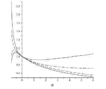
Figure 1. Bounds $r(x)A_{1}(x)$, $r(x)B_{1}(x)$ (bold line) and $r(x)A_{2}^{\pm}(x)$, $r(x)B_{2}^{\pm}(x)$ (dashed line) for $x\in(-0.9,6)$, $g_{1}=0.7$, $g_{2}=0.3$, $r(x)=\sqrt{1+x}$.

Let us put $g_{1}=0.7$, $g_{2}=0.3$ so that the rational bounds of order $1$ and $2$ given respectively by ($A_{1}$, $B_{1}$) and ( $A^{\pm}_{2}$, $B^{\pm}_{2}$) are defined. The Figure 1 illustrates then the mutual position of graphs of these functions, multiplied by $\sqrt{1+x}$ for $x\in(-0.9,6)$. As follows from Theorem 1.2, the approximation of order $2$ is more precise than the one given by order $1$.

The interesting link between $g$–fractions and probability theory was reported by Gerl [5]. One considers the nearest-neighbour random walks $X_{n}$, $n=0,1,2,...$ on $\mathbb{N}_{0}=\{0,1,2,...\}$ with the one-step transition probabilities $p_{i,k}=\mathrm{Prob}[X_{n+1}=k\mid X_{n}=i]$ defined by

$$p_{0,1}=1,\quad p_{j,j-1}=g_{j},\quad p_{j,j+1}=1-g_{j}\,$$ (1.30)

with $0<g_{j}<1$, $j\geq 1$ and $p_{j,k}=0$ in any other case.

We introduce $p_{0,0}^{2n}=\mathrm{Prob}[X_{2n}=0\mid X_{0}=0]$– the probability of return to $0$ in $2n$ steps. The generating function for this sequence

$$G_{0}(z)=\sum_{n=0}^{\infty}\,(-1)^{n}\,p_{0,0}^{2n}\,z^{n},\,$$ (1.31)

can be written then as a $g$–fraction:

$$G_{0}(z)=\{g_{1},g_{2},...|z\}\,.$$ (1.32)

Some other applications of $g$-fractions can be found in [15, 14, 16, 11].

In the next section we will examine the relation between $g$–fractions and real analytic bounded functions.

2. Functions bounded in the complex strip

We denote by $\mathbb{A}_{M,B}$ the set of functions $f(z)$ satisfying the following conditions

a) $f$ is holomorphic in the infinite strip $S_{B}=\{z\in\mathbb{C}\,:|\mathrm{Im}(z)|<B\}$ , $B>0$.

b) $f(\mathbb{R})\subset\mathbb{R}$.

c) $|f(z)|<M$, $M>0$, $\forall$ $z\in S_{B}$.

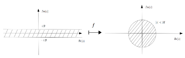
Figure 2. Map defined by $f\in\mathbb{A}_{M,B}.$

Our goal is to describe the $g$–fraction representation for the elements of $\mathbb{A}_{M,B}$ . Firstly, we note that it is sufficient to characterize only the functions from the class $\mathbb{A}_{1,\pi}$, since $f\in\mathbb{A}_{M,B}$ if and only if $\theta(z)=\frac{1}{M}{f(Bz}/{\pi})\in\mathbb{A}_{1,\pi}$. The answer is given by the following theorem

Theorem 2.1.

Let $\theta$ be a function holomorphic in the infinite complex strip $S=\{z\in\mathbb{C}\,:|\mathrm{Im}(z)|<\pi\}$, $|\theta(z)|<1$, $\forall\,z\in S$ and $\theta(\mathbb{R})\subset\mathbb{R}$. Then there exists a $g$-continued fraction

$$g(z)=\dfrac{1}{1}\begin{array}[]{cc}\\ +\end{array}\dfrac{g_{1}z}{1}\begin{array}[]{cc}\\ +\end{array}\dfrac{(1-g_{1})g_{2}z}{1}\begin{array}[]{cc}\\ +\end{array}\dfrac{(1-g_{2})g_{3}z}{1}\cdots\,,$$ (2.7)

with $g_{k}\in[0,1]$, $\forall\,k\geq 1$ such that

$$\theta(z)=1-\frac{2}{\mu\,e^{z/2}g(e^{z}-1)+1},\quad z\in S\,,$$ (2.8)

where $\mu=\displaystyle\frac{1+\theta(0)}{1-\theta(0)}$.

Proof.

We introduce the complex domains

$$\mathbb{D}=\{z\in\mathbb{C}\,:|z|<1\},\quad\mathbb{H}_{+}=\{z\in\mathbb{C}\,:\mathrm{Re}(z)>0\}\,,$$ (2.9)

and the conformal maps defined by:

$$m(z)=\frac{1+z}{1-z},\quad m\,:\mathbb{D}\to\mathbb{H}_{+}\,,$$ (2.10)

and

$$l(z)=\log(1+z),\quad l\,:\mathbb{H}\to S\,,$$ (2.11)

$$\eta(z)=l^{-1}(z)=e^{z}-1\,.$$ (2.12)

We note that $\eta$ is a bijection between $\mathbb{R}$ and $(-1,+\infty)$.

One verifies that the composition $F=m\circ f\circ l$ is holomorphic in $\mathbb{H}$ and $F(\mathbb{H})\subset\mathbb{H}_{+}$ with $F(z)\in\mathbb{R}$ for $z>-1$. Thus, according to theorem of Wall [17], p. 279 $F$ can be written as follows

$$F(z)=\mu\sqrt{1+z}\int_{0}^{1}\displaystyle\frac{d\mu(u)}{1+zu}\,,$$ (2.13)

for some nondecreasing real bounded function $\mu(u)$, $u\in(0,1)$ and $\mu>0$.

For $f=m^{-1}\circ F\circ\eta$ one obtains the following formula

$$f(z)=\left(1-\displaystyle\frac{2}{\mu e^{z/2}\int_{0}^{1}\displaystyle\frac{d\mu(u)}{1+(e^{z}-1)u}+1}\right).$$ (2.14)

The integral in (2.14) can be transformed to the continued $g$–fraction form [17]

$$\int^{1}_{0}\displaystyle\frac{d\mu(u)}{1+(e^{z}-1)u}=\left\{g_{1},g_{2},...|e^{z}-1\right\},\quad\mathrm{for\,\,some}\quad g_{k}\in[0,1]\,,$$ (2.15)

that together with (2.14) implies (2.8). End of proof. ∎

To calculate the coefficients $g_{p}$ in (2.7) one has formulas:

$$g_{p}=C_{p}(\theta(0),\theta^{\prime}(0),...,\theta^{(p)}(0)),\quad p\geq 1\,,$$ (2.16)

with rational functions $C_{p}$ determined by calculation of derivatives of both sides of (2.8) at $z=0$. The recurrent formulas for all $C_{p}$ can be derived from [17], p. 203.

Introducing

$$\theta_{n}=\theta^{(n)}(0),\quad n\geq 0\,,$$ (2.17)

we provide below explicit formulas for $g_{1}$ and $g_{2}$:

$$g_{1}=\frac{1}{2}\,\frac{1-4\theta_{1}-\theta_{0}^{2}}{1-\theta_{0}^{2}}\,,$$ (2.18)

$$g_{2}=\frac{1}{2}\frac{(16\theta_{1}^{2}-8\theta_{2}-\theta_{0}+\theta_{0}^{2}+\theta_{0}^{3}-8\theta_{2}\theta_{0}-1)(1-\theta_{0})}{(1-\theta_{0}^{2}+4\theta_{1})(4\theta_{1}-1+\theta_{0}^{2})}\,.$$ (2.19)

Our present aim is to estimate the time of return of $\theta\in\mathbb{A}_{1,\pi}$ to the initial value $\theta(0)$ i.e to study the real points $\tau\neq 0$ such that $\theta(\tau)=\theta(0)$. For this sake, we will use the a priori bounds (1.25) applied to the $g$–fraction in formula (2.8). For $p=2k+1$ one obtains:

$$\left(1-\displaystyle\frac{2}{\mu\sqrt{1+\eta(z)}A_{p}(\eta(z))+1}\right)\leq\theta(z)\leq\left(1-\displaystyle\frac{2}{\mu\sqrt{1+\eta(z)}B_{p}(\eta(z))+1}\right)\,,$$ (2.20)

for $z\in\mathbb{R}$.

If $p=2k$ then

$$\left(1-\displaystyle\frac{2}{\mu\sqrt{1+\eta(z)}A_{p}^{+}(\eta(z))+1}\right)\leq\theta(z)\leq\left(1-\displaystyle\frac{2}{\mu\sqrt{1+\eta(z)}B_{p}^{+}(\eta(z))+1}\right)\,,$$ (2.21)

for $z\in(0,+\infty)$, and

$$\left(1-\displaystyle\frac{2}{\mu\sqrt{1+\eta(z)}A_{p}^{-}(\eta(z))+1}\right)\leq\theta(z)\leq\left(1-\displaystyle\frac{2}{\mu\sqrt{1+\eta(z)}B_{p}^{-}(\eta(z))+1}\right)\,,$$ (2.22)

for $z\in(-\infty,0]$.

In the next theorem, for a given $f\in\mathbb{A}_{1,\pi}$, we will describe a neighborhood of origin in which $x=0$ is the only solution of $\theta(x)=\theta(0)$.

Theorem 2.2.

We assume that all conditions of the Theorem 2.1 are fulfilled and there exists a non zero $\tau\in\mathbb{R}$ such that $\theta(\tau)=\theta(0)$. Then $g_{1}(1-g_{1})\neq 0$ and the following inequality holds

$$|\tau|\geq 2\left|\log\frac{1-g_{1}}{g_{1}}\right|\,.$$ (2.23)

Proof.

One considers (2.20) with $p=1$. We have $A_{1}(0)=B_{1}(0)=1$ and define $t_{1}$, $t_{2}$ as non-zero solutions of the following algebraic equations

$$\sqrt{1+t_{1}}A_{1}(t_{1})=1,\quad\sqrt{1+t_{2}}B_{1}(t_{2})=1,\quad t_{1},t_{2}\in(-1,+\infty)\,.$$ (2.24)

Simple algebraic calculations show that the only solutions satisfying (2.24) are given by

$$t_{1}=\frac{1-2g_{1}}{g_{1}^{2}},\quad t_{2}=\frac{2g_{1}-1}{(1-g_{1})^{2}}\,,$$ (2.25)

which are related by

$$\frac{1}{t_{1}}+\frac{1}{t_{2}}=-1\,.$$ (2.26)

Since $\eta(z)$ is a bijection between $\mathbb{R}$ and $(-1,+\infty)$ there exist unique real numbers $T_{1}$, $T_{2}\in\mathbb{R}$ satisfying the following equations:

$$\eta(T_{1})=t_{1},\quad\eta(T_{2})=t_{2}\,.$$ (2.27)

As easily seen from (2.12): $T_{1}=-T_{2}$ and the proof of (2.23) follows straightforwardly from the formula (2.11). ∎

Remark 2.1.

It is easy to see that $g_{1}=1/2$ if and only if $\theta^{\prime}(0)=0$, as follows from (2.18). Hence, the right hand side of the inequality (2.23) is zero if $\theta^{\prime}(0)=0$, that corresponds to trivial case and is strictly positive if $\theta^{\prime}(0)\neq 0$.

The next result shows that $\theta\in\mathbb{A}_{1,\pi}$, under some conditions on derivatives $\theta^{(p)}(0)$, $p=0,1,2$, always returns to the initial value $\theta(0)$ i.e admits the oscillatory property.

Theorem 2.3.

Let $\theta\in\mathbb{A}_{1,\pi}$, $\theta^{\prime}(0)>0$ and $g_{1},g_{2}$ are defined by formulas (2.17) and (2.18), (2.19).

I.   We assume that the $(g_{1},g_{2})\in[0,1]^{2}$ belongs to one of the two regions $E$, $F$ defined by:

$$E=\{(g_{1},g_{2})\in(0,1)^{2}\,:\,D_{2}\geq 0,0<g_{1}<1/2,0<g_{2}<1/2\}\,,$$ (2.28)

$$F=\{(g_{1},g_{2})\in(0,1)^{2}\,:\,D_{2}\geq 0,0<g_{1}<1/2,1/2<g_{2}<1\}\,,$$ (2.29)

$$D_{1}=(1-g_{1})^{2}-4g_{1}^{2}g_{2}(1-g_{2}),\,D_{2}=g_{1}^{2}-4(1-g_{1})^{2}(1-g_{2})g_{2}\,.$$ (2.30)

Let

$$\zeta=\frac{2B}{\pi}\log(t^{(2)}_{1})>0\quad\mathrm{if}\quad(g_{1},g_{2})\in E$$ (2.31)

$$\zeta=\frac{2B}{\pi}\log(t^{(2)}_{2})<0\quad\mathrm{if}\quad(g_{1},g_{2})\in F$$ (2.32)

where $t^{(i)}_{j}$, $i,j=1,2$ are defined as functions of $g_{1},g_{2}$ by

$$t_{2,1}^{(1)}=\frac{1-g_{1}\pm\sqrt{D_{1}}}{2g_{1}(1-g_{2})},\quad t_{2,1}^{(2)}=\frac{g_{1}\pm\sqrt{D_{2}}}{2(1-g_{1})g_{2}}\,.$$ (2.33)

Then there exists $\tau\in\mathbb{R}$, $\tau\neq 0$ such that

$$\theta(\tau)=\theta(0)\,,$$ (2.34)

and

$$\tau\in(0,\zeta)\,\quad\mathrm{if}\quad\zeta>0\quad\mathrm{and}\quad\tau\in(\zeta,0)\quad\mathrm{if}\quad\zeta<0\,.$$ (2.35)

II.   Let $\tau\in\mathbb{R}$, $\tau\neq 0$ be such that $\theta(\tau)=\theta(0)$, then

$$\tau\in(-\infty,\frac{2B}{\pi}\log(t_{1}^{(1)})]\cup[\frac{2B}{\pi}\log(t_{2}^{(1)}),+\infty)\,.$$ (2.36)

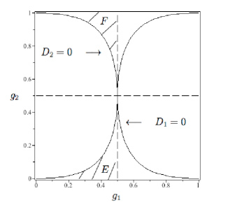
Figure 3. Domains $E$, $F$ in the parameter space $(g_{1},g_{2})\in[0,1]^{2}$.

Proof.

We consider (2.21) with $p=2$ and define the following real algebraic equations

$$\sqrt{1+x}\,A_{2}^{+}(x)=1\,,\quad x\in(0,+\infty)\,,\quad\mathrm{(A_{1})}\,,$$

$$\sqrt{1+x}\,B_{2}^{+}(x)=1\,,\quad x\in(0,+\infty)\,,\quad\mathrm{(B_{1})}\,,$$

$$\sqrt{1+x}\,B_{2}^{-}(x)=1\,,\quad x\in(-1,0)\,,\quad\mathrm{(\tilde{A}_{1})}\,,$$

$$\sqrt{1+x}\,A_{2}^{-}(x)=1\,,\quad x\in(-1,0)\,.\quad\mathrm{(\tilde{B}_{1})}\,,$$

where $A_{2}^{-}=B_{2}^{+}$, $B_{2}^{-}=A_{2}^{+}$.

Making the change of variables

$$x=-1+t^{2},\quad t\in\mathbb{R}\,,$$ (2.37)

after some elementary transformations, it is easy to show that equations ($A_{1}$), ($B_{1}$) are equivalent respectively to quadratic equations ($A_{2}$) and ($B_{2}$) given below

$$P_{1}(t)=g_{1}(1-g_{2})t^{2}-(1-g_{1})t+g_{1}g_{2}=0,\quad t\in\mathbb{R},\quad\mathrm{(A_{2})}$$

$$P_{2}(t)=g_{2}(1-g_{1})t^{2}-g_{1}t+(1-g_{1})(1-g_{2})=0,\quad t\in\mathbb{R}\,.\quad\mathrm{(B_{2})}$$

Remark 2.2.

We notice that $P_{2}(t)$ is obtained from $P_{1}(t)$ by transformation

$$g_{i}\mapsto 1-g_{i},\quad i=1,2\,.$$ (2.38)

The polynomial $P_{1}(t)=0$ has two real roots $t_{1}^{(1)},t_{2}^{(1)}\in\mathbb{R}$

$$t_{1}^{(1)}=\frac{1-g_{1}-\sqrt{D_{1}}}{2g_{1}(1-g_{2})},\quad t_{2}^{(1)}=\frac{1-g_{1}+\sqrt{D_{1}}}{2g_{1}(1-g_{2})},\quad t_{1}^{(1)}\leq t_{2}^{(1)}\,,$$ (2.39)

if and only if the following condition holds

$$D_{1}=(1-g_{1})^{2}-4g_{1}^{2}g_{2}(1-g_{2})\geq 0\,.$$ (2.40)

$P_{2}(t)=0$ has two real solutions $t_{1}^{(2)},t_{2}^{(2)}\in\mathbb{R}$

$$t_{1}^{(2)}=\frac{g_{1}-\sqrt{D_{2}}}{2(1-g_{1})g_{2}},\quad t_{2}^{(2)}=\frac{g_{1}+\sqrt{D_{2}}}{2(1-g_{1})g_{2}},\quad t_{1}^{(2)}\leq t_{2}^{(2)}\,,$$ (2.41)

if and only if

$$D_{2}=g_{1}^{2}-4(1-g_{1})^{2}(1-g_{2})g_{2}\geq 0\,.$$ (2.42)

Applying the Vieta’s formulas to polynomials $A_{2}$ and $B_{2}$, and taking into account that $g_{i}\in(0,1)$, $i=1,2$ one checks that:

$$t^{(i)}_{j}>0,\quad i,j=1,2\,.$$ (2.43)

Let $f^{\prime}(0)>0(\Leftrightarrow g_{1}<1/2$). Then $\theta(z)$ is increasing function in the interval $(-\epsilon,\epsilon)$ for some small $\epsilon>0$. We assume that inequality $D_{2}\geq 0$ holds, so both roots $t^{(2)}_{1}$ and $t^{(2)}_{2}$ are real. One has $P_{2}(1)=1-2g_{1}>0$, so, in view of (2.43), either

$$0<t^{(2)}_{1}\leq t^{(2)}_{2}<1$$

or

$$1<t^{(2)}_{1}\leq t^{(2)}_{2}$$

One verifies with help of (2.41) that (a) is equivalent to

$$L_{2}=g_{1}-2(1-g_{1})g_{2}<0$$

and (b) to $L_{2}>0$.

Thus, in view of (2.37), if (b) holds, the equation ($B_{1}$) will have solution

$$x=-1+{t^{(2)}_{1}}^{2}\in(0,+\infty)\,,$$

and if (a) holds, ($\tilde{B}_{1}$) will have solution

$$x=-1+{t^{(2)}_{2}}^{2}\in(-1,0)\,,$$

in view of (2.37).

One verifies directly that the condition $0<g_{1}<1/2$ implies $D_{1}>0$.

So, the both roots $t_{1}^{(1)}$ and $t_{2}^{(1)}$ are real distinct numbers.

Since $P_{1}(1)=2g_{1}-1<0$ we have $0<t_{1}^{(1)}<1<t_{2}^{(1)}$. So, the equation ($A_{1}$) will have the unique real solution

$$y_{2}=-1+{t_{2}^{(1)}}^{2}\in(0,+\infty)\,,$$ (2.44)

and ($\tilde{A}_{1}$) will have the unique real solution

$$y_{1}=-1+{t_{1}^{(1)}}^{2}\in(-1,0)\,.$$ (2.45)

Since $\eta(z)$ is a bijection of $\mathbb{R}$ and $(-1,+\infty)$, there exists unique real number $\zeta\in\mathbb{R}$ satisfying equation $\eta(\zeta)=x$ with $x\in(-1,+\infty)$ defined above. Then, as follows from (2.21), (2.22), there exists $\tau$ satisfying (2.34) if one of the cases (2.28)-(2.29) holds. One has $\tau\in(0,\zeta)$ if $\zeta>0$ and $\tau\in(\zeta,0)$ if $\zeta<0$.

Using $y_{1,2}$ defined above, we define $z_{1}<0$ and $z_{2}>0$ as unique real solutions of $\eta(z_{i})=y_{i}$, $i=1,2$. Let now $\tau\neq 0$ be such that $\theta(\tau)=\theta(0)$, then $\tau\in(-\infty,z_{1}]\cup[z_{2},+\infty)$ that shows (2.36) and finishes the proof.

∎

The case $\theta^{\prime}(0)<0$ can be analyzed in the similar way by considering $\theta(-z)$ instead of $\theta(z)$.

3. Applications to solutions of the $ABC$–flow equations

The $ABC$–flow is a system of three ordinary differential equations

$$\frac{dx_{1}}{dz}=A\sin x_{3}+C\cos x_{2},\quad\frac{dx_{2}}{dz}=B\sin x_{1}+A\cos x_{3},\quad\frac{dx_{3}}{dz}=C\sin x_{2}+B\cos x_{1}\,,$$ (3.1)

depending on three arbitrary real positive constants $(A,B,C)\neq(0,0,0)$.

This vector field appears as an exact solution of the Euler equation without forcing. It is essential to the origin of magnetic fields in large astrophysical bodies like the Earth, the Sun and galaxies. The history of the problem, including numerous applications, can be found in [4], [1]. Through intensive numerical studies [3], [18], [7], it was shown that the dynamics of the $ABC$-flow is generally chaotic. In particular, it means that, due to exponential instability of its solutions, any kind of a long time prediction of evolutionary dynamics is problematic.

The rigorous study of integrability, that is of the existence of conservation lows (first integrals) of the $ABC$-flow was initiated by Ziglin in the cycle of papers [19]-[21]. Applying the complex analytic monodromy approach, he proved that the $ABC$-flow does not have any non constant meromorphic first integrals. The results of Ziglin have been generalized and extended later in [9] based on the more recent differential Galois approach of Morales-Ramis (see [10] for details).

The purpose of our study is to elaborate on the idea that some qualitative insight into dynamics of the $ABC$–flow can be gained using the $g$-fractions approach. More precisely, we aim to establish analytically the existence of the recurrent behavior (Theorem 3.2).

We define

$$\delta=\max\{A+C,B+A,C+B\}>0\,.$$ (3.2)

Since the vector field of (3.1) is a bounded one it is complete in $\mathbb{R}^{3}$ and hence all its real solutions $(x_{1}(z),x_{2}(z),x_{3}(z))$ are defined for $z\in\mathbb{R}$. We will need the following elementary property, easy to proof

Proposition 3.1.

The trigonometric functions $\cos x$, $\sin x$ are analytic and bounded in absolute value by $\mathrm{ch}(\epsilon)$ in the complex disk $|x-x_{0}|<\epsilon$ with a center $x_{0}\in\mathbb{R}$.

And we remind the classical theorem of Picard (see for example [12]) from the analytic theory of ordinary differential equations:

Theorem 3.1.

(Picard [12]) Let $Q_{j}(q_{1},q_{2},\dots,q_{n})$, $1\leq j\leq n$ be analytic functions in the complex domain

$$|q_{i}-\bar{q}_{i}|<q^{\prime}_{i},\quad 1\leq i\leq n\,,$$ (3.3)

for some $q^{\prime}_{i}>0$, $\bar{q}_{i}\in\mathbb{C}$, $1\leq i\leq n$. We assume that there exist positive constants $Q^{\prime}_{j}>0$, $1\leq j\leq n$ such that

$$|Q_{j}(q_{1},q_{2},\dots,q_{n})|<Q^{\prime}_{j},\quad 1\leq j\leq n\,,$$ (3.4)

if the conditions (3.3) hold.

Then the system of $n$ ordinary equations

$$\frac{dq_{j}}{dz}=Q_{j}(q_{1},q_{2},\dots,q_{n}),\quad 1\leq j\leq n\,,$$ (3.5)

admits the unique solution analytic in the complex disc

$$D\,:\,|z|<T^{\prime},\quad T^{\prime}=\mathrm{min}\left\{\frac{q^{\prime}_{1}}{Q^{\prime}_{1}},\frac{q^{\prime}_{2}}{Q^{\prime}_{2}},\dots,\frac{q^{\prime}_{n}}{Q^{\prime}_{n}}\right\}\,,$$ (3.6)

satisfying the initial conditions $q_{i}(0)=\bar{q}_{i}$, $1\leq i\leq n$.

Moreover,

$$|q_{i}(z)-\bar{q}_{i}|<q^{\prime}_{i},\quad z\in D,\quad 1\leq i\leq n\,.$$ (3.7)

Our first result is given by the following theorem

Lemma 3.1.

Let $\epsilon>0$ be an arbitrary positive real number. Then every real solution $(x_{1}(z),x_{2}(z),x_{3}(z))$ of (3.1) is an analytic function of $z$ in the complex infinite strip

$$S_{b}=\{z\in\mathbb{C}\,:\,|\mathrm{Im}(z)|<b\},\quad b=\frac{1}{\delta}\,\frac{\epsilon}{\mathrm{ch}(\epsilon)}\,.$$ (3.8)

Proof.

For a given $\epsilon>0$ and a real triplet $(X_{1},X_{2},X_{3})\in\mathbb{R}^{3}$, we introduce the complex domain $\mathcal{D}_{X_{1},X_{2},X_{3}}^{\epsilon}=\{(x_{1},x_{2},x_{3})\in\mathbb{C}^{3}\,:\,|x_{i}-X_{i}|<\epsilon,\,i=1,2,3\}$. Writing the system (3.1) in the form $\dot{x}_{i}=f_{i}(x_{1},x_{2},x_{3})$, $i=1,2,3$ one easily verifies that

$$|f_{i}(P)|<\delta\,\mathrm{ch}(\epsilon),\quad\forall\,P=(x_{1},x_{2},x_{3})\in{\mathcal{D}_{X_{1},X_{2},X_{3}}^{\epsilon}},\quad 1\leq i\leq 3\,,$$ (3.9)

in view of Proposition 3.1.

According to the Picard’s Theorem 3.1, the solution of (3.1) $z\mapsto(x_{1}(z),x_{2}(z),x_{3}(z))$, defined by the initial condition $(x_{1}(z_{0}),x_{2}(z_{0}),x_{3}(z_{0}))=(X_{1},X_{2},X_{3})$, $z_{0}\in\mathbb{R}$, will be analytic in the disk $D_{z_{0},T^{\prime}}\,:\,|z-z_{0}|<T^{\prime}$ of the complex time plane with $T^{\prime}=\displaystyle\frac{\epsilon}{\delta\,\mathrm{ch}(\epsilon)}$. Since the system (3.1) is autonomous and $S_{b}=\cup_{z_{0}\in\mathbb{R}}\,D_{z_{0},T^{\prime}}$ that finishes the proof.

∎

Remark 3.1.

The function $e(\epsilon)=\epsilon/\mathrm{ch}(\epsilon)$ reaches the unique maximal value for $\epsilon\in\mathbb{R}_{+}$ which we denote $e_{max}$. The direct computation gives $e_{max}=e(\epsilon_{max})=0.6627$ for $\epsilon_{max}=1.1997$.

The solutions of the $ABC$–flow are defined on the torus $\mathbb{T}^{3}=\{(x_{1},x_{2},x_{3})\,:\,x_{i}\,\mathrm{mod}\,2\pi\}$. We aim now to study the projections $\phi_{i}\,:\,\mathbb{R}\to[-1,1]$ defined by

$$\phi_{i}(z)=\sin(x_{i}(z)/2),\quad i=1,2,3\,.$$ (3.10)

These functions are of dynamical importance since the sections $x_{i}=0\mod 2\pi$ in $\mathbb{T}^{3}$ can be viewed as the zero level surfaces $\phi_{i}=0$. Indeed, since $x_{i}(z)\in[0,2\pi]$ the only solutions of the equation $\phi_{i}(z)=\sin(x_{i}(z)/2)=0$ is given by $x_{i}(z)=0\mod 2\pi$.

Lemma 3.2.

Let $z\in\mathbb{R}\mapsto(x_{1}(z),x_{2}(z),x_{3}(z))$ be an arbitrary real solution of the $ABC$–flow (3.1). Then all functions $\phi_{i}(z)=\sin(x_{i}(z)/2)$, $i=1,2,3$ are analytic in $S_{b}$ defined by (3.8) and bounded in absolute value by $M=\mathrm{ch}(\epsilon/2)$.

Proof.

Let $x_{j}(z)\in(x_{1}(z),x_{2}(z),x_{3}(z))$. Then, $\phi_{j}(z)=\sin(x_{j}(z))$ is analytic in $S_{b}$ as a composition of analytic maps. Let $z_{0}\in\mathbb{R}$, then for the complex disc $D_{z_{0},b}\,:\,|z-z_{0}|<b$ we have obviously $D_{z_{0},b}\subset S_{b}$. According to (3.7) $\forall\,z\in D_{z_{0},b}\,:\,|x_{j}(z)-x_{j}(z_{0})|<\epsilon$. That completes the proof in view of $S_{b}=\cup_{z_{0}\in\mathbb{R}}\,D_{z_{0},b}$ and Proposition 3.1.

∎

We consider an arbitrary solution $\Gamma_{\alpha,\beta}$ of (3.1) starting from the plane $x_{1}=0\mod 2\pi$, and defined by initial conditions of the form

$$x_{1}(0)=0,\quad x_{2}(0)=\alpha,\quad x_{3}(0)=\beta,\quad\alpha,\beta\in[0,2\pi]\,.$$ (3.11)

Let $f(z)=\phi_{1}(z)=\sin(x_{1}(z)/2)$. We have $f(0)=0$, $f\in\mathbb{A}_{M,b}$ and the formulas (2.17), (2.18), (2.19) give

$$\theta_{0}=0,\quad\theta_{1}=\frac{1}{2\pi\delta}\,\frac{\epsilon}{\mathrm{ch}(\epsilon)\mathrm{ch}(\epsilon/2)}(A\sin\beta+C\cos\alpha),\quad\theta_{2}=\frac{1}{2\pi^{2}\delta^{2}}\,\frac{\epsilon^{2}}{\mathrm{ch}^{2}\mathrm{ch}(\epsilon)(\epsilon/2)}AB\cos\beta\,,$$ (3.12)

and

$$g_{1}=\frac{1}{2}\left(1-4\theta_{1}\right),\quad g_{2}=\frac{1}{2}\left(1+\frac{8\theta_{2}}{1-16\theta_{1}^{2}}\right)\,.$$ (3.13)

Since $f\in\mathbb{A}_{M,b}$, according to Theorem 2.1 we have $g_{1,2}\in[0,1]$. One easily verifies that the strict inequalities always hold: $0<g_{1,2}<1$. Let $\tau\neq 0$ be such that $x_{1}(\tau)=0\mod 2\pi$. According to Theorem 2.2 we have the following explicit lower bound

$$|\tau|\geq\frac{4\,\epsilon}{\pi\,\delta\,\mathrm{ch}(\epsilon)}\mathrm{arctanh}\left(\frac{2\,\epsilon}{\pi\,\delta\,\mathrm{ch}(\epsilon/2)\mathrm{ch}(\epsilon)}(A\sin\beta+C\cos\alpha)\right)\,,$$ (3.14)

which is true for any $(\alpha,\beta)\in[0,2\pi]^{2}$ and arbitrary $\epsilon>0$, $\delta$ is defined by (3.2).

From the dynamical point of view, this means that the solution $\Gamma_{\alpha,\beta}$ leaving the plane $x_{1}=0$, can not return back earlier than permitted by (3.14). In practice, one can use a freedom in the chose of $\epsilon$ in order to make (3.14) optimal. The more precise lower bound, involving $g_{2}$ i.e the second derivative of $f$ at $0$, is given by (2.36). The corresponding to (3.14) formula is straightforward to obtain.

Now we will analyze the upper bound on $\tau$ given by Theorem 2.3 assuming that $\dot{x}_{1}(0)>0\Leftrightarrow g_{1}<1/2$.

The condition (2.28) defines the region $E$ in the parameter space $(\alpha,\beta)\in[0,2\pi]^{2}$ and is equivalent to the system of inequalities

$$\theta_{1}>0,\quad\theta_{2}\leq-\frac{\sqrt{\theta_{1}}}{2}(1-4\theta_{1})\,.$$ (3.15)

One can show that for any positive constants $A,B,C$ and $\epsilon$ the above set of parameter values $(\alpha,\beta)$ is non empty in $[0,2\pi]^{2}$ . Indeed, it is sufficient to put $\alpha=\pi/2$ in (3.12) and consider the values ($\beta\to\pi$, $\beta<\pi$) to satisfy (3.15). Therefore, by the continuity argument, we can state the following

Theorem 3.2.

The Poincaré section $\Pi=\{(x_{1},x_{2},x_{3})\in\mathbb{T}^{3}\,|\,x_{1}=0\mod 2\pi\}$ of the $ABC$–flow (3.1) contains a positive measure set of initial conditions $(\alpha,\beta)$ for which the solutions $\Gamma_{\alpha,\beta}$ return to $\Pi$.

The corresponding upper bounds for the time of return $\tau$ can be calculated with help of (2.31).

4. Conclusion

The presented work was motivated by the ideas of Poincaré and Sundman [2] from the Celestial Mechanics providing converging time series solutions for the $3$–body problem. These ones follows from the analyticity of regularized collision free solutions in the infinite complex strip of the time plane. Unfortunately, these series, though existing for all values of time, have very slow convergence. One would have to sum up milliards of terms to gain any significant qualitative information above the motion of particles. The present study was designed to test the hypothesis that this gap can be overcome by replacing the power series with functional continued fractions. We notice that this issue has not yet been addressed fully in the literature and a number of aspects of the $g$–fractions approach presented here require further investigation. As a toy model, we consider the $ABC$–flow system (3.1) exhibiting the chaotic behavior. In particular, this system can not be solved by quadratures and being non–integrable, does not have any globally defined analytic conservation laws. Nevertheless, as shown by Lemma 3.2, all solutions of this system belong to the class of real analytic bounded functions and thus admit the $g$–fraction representation as stated by Theorem 2.1. Applying the rational approximation, we can derive the upper and lower bounds on the time of the first return for a Poincaré map of the $ABC$-flow which was defined in Section 3. As a conclusion, we establish by Theorem 3.2 the existence of a non empty set of trajectories of the $ABC$–flow, exhibiting the recurrent behavior.

5. Acknowledgments

The author is grateful to anonymous referees for their useful remarks and suggestions.

References

[1] P. Ashwin, O. Podvigina, Hopf bifurcation with cubic symmetry and instability of ABC flow, Proc. Roy. Soc. London. 459, 1801–1827, 2003.
[2] F. Diacu, The solution of the n-body problem, The Mathematical Intelligencer 18 (3), 66-70, 1996.
[3] T. Dombre, U. Frisch, J. M. Greene, M. Hénon, A. Mehr, A.M. Soward, Chaotic streamlines in the ABC flows, J. Fluid Mech. 167, 353?391, 1986
[4] D. Galloway, flows then and now, Geophysical & Astrophysical Fluid Dynamics Volume 106, Issue 4-5, 2012.
[5] P. Gerl, Continued fraction method for random walks on and on trees , Probability Measures on Groups, Proceedings, Oberwolfach, 1983, Lecture Notes in Mathematics, 1064, Springer-Verlag, Berlin, 131-146.
[6] W. B. Gragg, Truncation error bounds for -fractions , Numerische Mathematik, 11, pp. 370-379, 1968.
[7] De-Bin Huanga, Xiao-Hua Zhaoa, Hui-Hui Daib, Invariant tori and chaotic streamlines in the ABC flow, Physics Letters A, Volume 237, Issue 3, 5, 136?140, 1998
[8] R. Kustner, Mapping Properties of Hypergeometric Functions and Convolutions of Starlike or Convex Functions of Order , Computational Methods and Function Theory, Volume 2, (2002), No. 2, 597 610.
[9] A. J. Maciejewski, M. Przybylska, Non-integrability of ABC flow, Phys. Lett. A 303, 265?272, 2002.
[10] J.J. Morales Ruiz, Differential Galois Theory and Non-Integra-
bility of Hamiltonian Systems, Birkh user, Basel, 1999.
[11] B.D. Mestel, A.H. Osbaldestin, A. Tsygvintsev, Bounds on the unstable eigenvalue for the asymmetric renormalization operator for period doubling, Communications in Mathematical Physics, Volume 250, Number 2, 2004, 241-257.
[12] E. Picard, Traité d’analyse, Jacques Gabay, Sceaux, T. 2, Ch. 9, 1991.
[13] K.F. Sundman, Mémoire sur le probleème des trois corps, Acta math- ematica, 36, p. 105-179, 1912.
[14] A. Tsygvintsev, On the convergence of continued fractions at Runckel’s points, The Ramanujan Journal, Vol. 15, No. 3, 2008,407-413.
[15] A. Tsygvintsev, On the connection between –fractions and solutions of the Feigenbaum-Cvitanovic equation, Commun, in the Analytic Theory of Continued Fractions, Vol. XI, 2003, 103-112.
[16] A. Tsygvintsev, B.D. Mestel, A.H. Osbaldestin, Continued fractions and solutions of the Feigenbaum-Cvitanovic equation, C.R. Acad. Sci. Paris, t. 334, S rie I, 2002, 683-688.
[17] H. S. Wall, Analytic Theory of Continued Fractions, D. Van Nostrand Company, Inc., New York, N. Y., 1948.
[18] Xiao-Hua Zhao, Keng-Huat Kwek, JI-Bin Li, Ke-Lei Huang, Chaotic and Resonant Streamlines in the Flow, SIAM J. Appl. Math., 53(1), 71?77, 1993
[19] S. L. Ziglin, The -flow is not integrable for , Funkts. Anal. Prilozh., Volume 30, Issue 2, 80-81, 1996.
[20] S. L. Ziglin, On the absence of a real-analytic first integral for flow when , Chaos 8, 272-273, 1998.
[21] S. L. Ziglin, An analytic proof of the nonintegrability of the -flow for , Funct. Anal. Appl. 3, 225-227, 2003