An Efficient Dual Approach to
Distance Metric Learning

Abstract

Distance metric learning is of fundamental interest in machine learning because the distance metric employed can significantly affect the performance of many learning methods. Quadratic Mahalanobis metric learning is a popular approach to the problem, but typically requires solving a semidefinite programming (SDP) problem, which is computationally expensive. Standard interior-point SDP solvers typically have a complexity of $O(D^{6.5})$ (with $D$ the dimension of input data), and can thus only practically solve problems exhibiting less than a few thousand variables. Since the number of variables is $D(D+1)/2$, this implies a limit upon the size of problem that can practically be solved of around a few hundred dimensions. The complexity of the popular quadratic Mahalanobis metric learning approach thus limits the size of problem to which metric learning can be applied. Here we propose a significantly more efficient approach to the metric learning problem based on the Lagrange dual formulation of the problem. The proposed formulation is much simpler to implement, and therefore allows much larger Mahalanobis metric learning problems to be solved. The time complexity of the proposed method is $O(D^{3})$, which is significantly lower than that of the SDP approach. Experiments on a variety of datasets demonstrate that the proposed method achieves an accuracy comparable to the state-of-the-art, but is applicable to significantly larger problems. We also show that the proposed method can be applied to solve more general Frobenius-norm regularized SDP problems approximately.

I Introduction

Distance metric learning has attracted a lot of research interest recently in the machine learning and pattern recognition community due to its wide applications in various areas [1, 2, 3, 4]. Methods relying upon the identification of an appropriate data-dependent distance metric have been applied to a range of problems, from image classification and object recognition, to the analysis of genomes. The performance of many classic algorithms such as $k$-nearest neighbor ($k$NN) and $k$-means clustering depends critically upon the distance metric employed.

Large-margin metric learning is an approach which focuses on identifying a metric by which the data points within the same class lie close to each other and those in different classes are separated by a large margin. Weinberger et al.’s large-margin nearest neighbor (LMNN) [1] is a seminal work illustrating the approach whereby the metric takes the form of a Mahanalobis distance. Given input data ${\boldsymbol{a}}\in\mathbb{R}^{D}$, this approach to the metric learning problem can be framed as that of learning the linear transformation ${\mathbf{L}}$ which optimizes a criterion expressed in terms of Euclidean distances amongst the projected data ${\mathbf{L}}{\boldsymbol{a}}\in\mathbb{R}^{d}$.

In order to obtain a convex problem, instead of learning the projection matrix (${\mathbf{L}}\in\mathbb{R}^{D\times d}$), one usually optimizes over the quadratic product of the projection matrix (${\mathbf{X}}={\mathbf{L}}{\mathbf{L}}^{\!\top}$) [3, 1]. This linearization convexifies the original non-convex problem. The projection matrix may then be recovered by an eigen-decomposition or Cholesky decomposition of ${\mathbf{X}}$.

Typical methods that learn the projection matrix ${\mathbf{L}}$ are most of the spectral dimensionality reduction methods such as principle component analysis (PCA), Fisher linear discriminant analysis (LDA); and also neighborhood component analysis (NCA) [5], relevant component analysis (RCA) [6]. Goldberger et al. showed that NCA may outperform traditional dimensionality reduction methods [5]. NCA learns the projection matrix directly through optimization of a non-convex objective function. NCA is thus prone to becoming trapped in local optima, particularly when applied to high-dimensional problems. RCA [6] is an unsupervised metric learning method. RCA does not maximize the distance between different classes, but minimizes the distance between data in Chunklets. Chunklets consist of data that come from the same (although unknown) class.

More methods on the topic of large-margin metric learning actually learn ${\mathbf{X}}$ directly since Xing et al. [3] proposed a global distance metric learning approach using a convex optimization method. Although the experiments in [3] show improved performance on clustering problems, this is not the case when the method is applied to most classification problems. Davis et al. [7] proposed an information theoretic metric learning (ITML) approach to the problem. The closest work to ours may be LMNN [1] and BoostMetric [8]. LMNN is a Mahanalobis metric form of $k$-NN whereby the Mahanalobis metric is optimized such that the $k$-nearest neighbors are encouraged to belong to the same class while data points from different classes are separated by a large margin. The optimization take the form of an SDP problem. In order to improve the scalability of the algorithm, instead of using standard SDP solvers, Weinberger et al. [1] proposed an alternating estimation and projection method. At each iteration, the updated estimate ${\mathbf{X}}$ is projected back to the semidefinite cone using eigen-decomposition, in order to preserve the semi-definiteness of ${\mathbf{X}}$. In this sense, at each iteration, the computational complexity of their algorithm is similar to that of ours. However, the alternating method needs an extremely large number of iterations to converge (the default value being $10,000$ in the authors’ implementation). In contrast, our algorithm solves the corresponding Lagrange dual problem and needs only $20\sim 30$ iterations in most cases. In addition, the algorithm we propose is significantly easier to implement.

As pointed in these earlier work, the disadvantage of solving for ${\mathbf{X}}$ is that one needs to solve a semidefinite programming (SDP) problem since ${\mathbf{X}}$ must be positive semidefinite (p.s.d.). Conventional interior-point SDP solvers have a computation complexity of $O(D^{6.5})$, with $D$ the dimension of input data. This high complexity hampers the application of metric learning to high-dimensional problems.

To tackle this problem, here we propose here a new formulation of quadratic Mahalanobis metric learning using proximity comparison information and Frobenius norm regularization. The main contribution is that, with the proposed formulation, we can very efficiently solve the SDP problem in the dual space. Because strong duality holds, we can then recover the primal variable ${\mathbf{X}}$ from the dual solution. The computational complexity of the optimization is dominated by eigen-decomposition, which is $O(D^{3})$ and thus the overall complexity is $O(t\cdot D^{3})$, where $t$ is the number of iterations required for convergence. Note that $t$ does not depend on the size of the data, and is typically $t\approx 20\sim 30$.

A number of methods exist in the literature for large-scale p.s.d. metric learning. Shen et al. [8, 9] introduced BoostMetric by adapting the boosting technique, typically applied to classification, to distance metric learning. This work exploits an important theorem which shows that a positive semidefinite matrix with trace of one can always be represented as a convex combination of multiple rank-one matrices. The work of Shen et al. generalized LPBoost [10] and AdaBoost by showing that it is possible to use matrices as weak learners within these algorithms, in addition to the more traditional use of classifiers or regressors as weak learners. The approach we propose here, FrobMetric, is inspired by BoostMetric in the sense that both algorithms use proximity comparisons between triplets as the source of the training information. The critical distinction between FrobMetric and BoostMetric, however, is that reformulating the problem to use the Frobenius regularization—rather than the trace norm regularization—allows the development of a dual form of the resulting optimization problem which may be solved far more efficiently. The BoostMetric approach iteratively computes the squared Mahalanobis distance metric using a rank-one update at each iteration. This has the advantage that only the leading eigenvector need be calculated, but leads to slower convergence. Indeed, for BoostMetric, the convergence rate remains unclear. The proposed FrobMetric method, in contrast, requires more calculations per iteration, but converges in significantly fewer iterations. Actually in our implementation, the convergence rate of FrobMetric is guaranteed by the employed Quasi-Newton method.

The main contributions of this work are as follows.

1. We propose a novel formulation of the metric learning problem, based on the application of Frobenius norm regularization.

2. We develop a method for solving this formulation of the problem which is based on optimizing its Lagrange dual. This method may be practically applied to a much more complex datasets than the competing SDP approach, as it scales better to large databases and to high dimensional data.

3. We generalize the method such that it may be used to solve any Frobenius norm regularized SDP problem. Such problems have many applications in machine learning and computer vision, and by way of example we show that it may be used to approximately solve the Frobenius norm perturbed maximum variance unfolding (MVU) problem [11]. We demonstrate that the proposed method is considerably more efficient than the original MVU implementation on a variety of data sets and that a plausible embedding is obtained.

The proposed scalable semidefinite optimization method can be viewed as an extension of the work of Boyd and Xiao [12]. The subject of Boyd and Xiao in [12] was similarly a semidefinite least-squares problem: finding the covariance matrix that is closest to a given matrix under the Frobenius norm metric. Here we study the large-margin Mahalanobis metric learning problem, where, in contrast, the objective function is not a least squares fitting problem. We also discuss, in Section III the application of the proposed approach to general SDP problems which have Frobenius norm regularization terms. Note also that a precursor to the approach described here also appeared in [13]. Here we have provided more theoretical analysis as well as experimental results.

In summary, we propose a simple, efficient and scalable optimization method for quadratic Mahalanobis metric learning. The formulated optimization problem is convex, thus guaranteeing that the global optimum can be attained in polynomial time [14]. Moreover, by working with the Lagrange dual problem, we are able to use off-the-shelf eigen-decomposition and gradient descent methods such as L-BFGS-B to solve the problem.

I-A Notation

A column vector is denoted by a bold lower-case letter ($\boldsymbol{x}$) and a matrix is by a bold upper-case letter (${\mathbf{X}}$). The fact that a matrix ${\mathbf{A}}$ is positive semidefinite (p.s.d.) is denoted thus ${\mathbf{A}}\succcurlyeq 0$. The inequality ${\mathbf{A}}\succcurlyeq{\mathbf{B}}$ is intended to indicate that ${\mathbf{A}}-{\mathbf{B}}\succcurlyeq 0$. In the case of vectors, ${\boldsymbol{a}}\geq\boldsymbol{b}$ denotes the element-wise version of the inequality, and when applied relative to a scalar (e.g., ${\boldsymbol{a}}\geq 0$ ) the inequality is intended to apply to every element of the vector. For matrices, we denote by $\mathbb{R}^{m\times n}$ the vector space of real matrices of size $m\times n$, and the space of real symmetric matrices as $\mathbb{S}$. Similarly, the space of symmetric matrices of size $n\times n$ is $\mathbb{S}^{n}$, and the space of symmetric positive semidefinite matrices of size $n\times n$ is denoted as $\mathbb{S}_{+}^{n}$. The inner product defined on these spaces is $\left<{\mathbf{A}},{\mathbf{B}}\right>=\operatorname{\bf Tr}({\mathbf{A}}^{\!\top}{\mathbf{B}})$. Here $\operatorname{\bf Tr}(\cdot)$ calculates the trace of a matrix. The Frobenius norm of a matrix is defined as $\bigl{\|}{\mathbf{X}}\bigr{\|}_{\mathrm{F}}^{2}=\operatorname{\bf Tr}({\mathbf{X}}{\mathbf{X}}^{\!\top})=\operatorname{\bf Tr}({\mathbf{X}}^{\!\top}{\mathbf{X}})$, which is the sum of all the squared elements of ${\mathbf{X}}$. $\operatorname{\bf diag}(\cdot)$ extracts the diagonal elements of a square matrix. Given a symmetric matrix ${\mathbf{X}}$ and its eigen-decomposition ${\mathbf{X}}={\mathbf{U}}{\boldsymbol{\Sigma}}{\mathbf{U}}^{\!\top}$ (${\mathbf{U}}$ being an orthonormal matrix, and ${\boldsymbol{\Sigma}}$ being real and diagonal), we define the positive part of ${\mathbf{X}}$ as

$$({\mathbf{X}})_{+}={\mathbf{U}}\Bigl{[}\max(\operatorname{\bf diag}({\boldsymbol{\Sigma}}),0)\Bigr{]}{\mathbf{U}}^{\!\top},$$

and the negative part of ${\mathbf{X}}$ as

$$({\mathbf{X}})_{-}={\mathbf{U}}\Bigl{[}\min(\operatorname{\bf diag}({\boldsymbol{\Sigma}}),0)\Bigr{]}{\mathbf{U}}^{\!\top}.$$

Clearly, ${\mathbf{X}}=({\mathbf{X}})_{+}+({\mathbf{X}})_{-}$ holds.

I-B Euclidean Projection onto the p.s.d. cone

Our proposed method relies on the following standard results, which can be found in textbooks such as Chapter 8 of [14]. The positive semidefinite part $({\mathbf{X}})_{+}$ of ${\mathbf{X}}$ is the projection of ${\mathbf{X}}$ onto the p.s.d. cone:

$$({\mathbf{X}})_{+}=\left\{\min_{\mathbf{Y}}\;\bigl{\|}{\mathbf{Y}}-{\mathbf{X}}\bigr{\|}_{\mathrm{F}}^{2},{\rm\;s.t.\;}{\mathbf{Y}}\succcurlyeq 0\right\}.$$ (1)

It is not difficult to check that, for any ${\mathbf{Y}}\succcurlyeq 0$,

$$\bigl{\|}{\mathbf{X}}-({\mathbf{X}})_{+}\bigr{\|}_{\mathrm{F}}^{2}=\bigl{\|}({\mathbf{X}})_{-}\bigr{\|}_{\mathrm{F}}^{2}\leq\bigl{\|}{\mathbf{X}}-{\mathbf{Y}}\bigr{\|}_{\mathrm{F}}^{2}.$$

In other words, although the optimization problem in (1) appears as an SDP programming problem, it can be simply solved by using eigen-decomposition, which is efficient. It is this key observation that serves as the backbone of the proposed fast method.

The rest of the paper is organized as follows. In Section II, we present the main algorithm for learning a Mahalanobis metric using efficient optimization. In Section III, we extend our algorithm to more general Frobenius norm regularized semidefinite problems. The experiments on various datasets are in shown Section IV and we conclude the paper in Section V.

II Large-margin Distance Metric Learning

We now briefly review quadratic Mahalanobis distance metrics. Suppose that we have a set of triplets $\SS=\{({\boldsymbol{a}}_{i},{\boldsymbol{a}}_{j},{\boldsymbol{a}}_{k})\}$, which encodes proximity comparison information. Suppose also that ${\bf dist}_{ij}$ computes the Mahalanobis distance between ${\boldsymbol{a}}_{i}$ and ${\boldsymbol{a}}_{j}$ under a proper Mahalanobis matrix. That is, ${\bf dist}_{ij}=\|{{\boldsymbol{a}}_{i}-{\boldsymbol{a}}_{j}}\|_{{\mathbf{X}}}^{2}=({\boldsymbol{a}}_{i}-{\boldsymbol{a}}_{j})^{\!\top}{\mathbf{X}}({\boldsymbol{a}}_{i}-{\boldsymbol{a}}_{j})$, where ${\mathbf{X}}\in\mathbb{S}_{+}^{D\times D}$, is positive semidefinite. Such a Mahanalobis metric may equally be parameterized by a projection matrix ${\mathbf{L}}$ where ${\mathbf{X}}={\mathbf{L}}{\mathbf{L}}^{\!\top}$.

Let us define the margin associated with a training triplet as $\rho_{r}=({\boldsymbol{a}}_{i}-{\boldsymbol{a}}_{k})^{\!\top}{\mathbf{X}}({\boldsymbol{a}}_{i}-{\boldsymbol{a}}_{k})-({\boldsymbol{a}}_{i}-{\boldsymbol{a}}_{j})^{\!\top}{\mathbf{X}}({\boldsymbol{a}}_{i}-{\boldsymbol{a}}_{j})={\left<{\mathbf{A}}_{r},{\mathbf{X}}\right>},$ with ${\mathbf{A}}_{r}=({\boldsymbol{a}}_{i}-{\boldsymbol{a}}_{k})({\boldsymbol{a}}_{i}-{\boldsymbol{a}}_{k})^{\!\top}-({\boldsymbol{a}}_{i}-{\boldsymbol{a}}_{j})({\boldsymbol{a}}_{i}-{\boldsymbol{a}}_{j})^{\!\top}$. Here $r$ represents the index of the current triplet within the set of $m$ training triplets $\SS$. As will be shown in the experiments below, this type of proximity comparison among triplets may be easier to obtain that explicit distances for some applications like image retrieval. Here the metric learning procedure solely relies on the matrices ${\mathbf{A}}_{r}$ ($r=1,\dots,m$).

II-A Primal problems of Mahanalobis metric learning

Putting it into the large-margin learning framework, the optimization problem is to maximize the margin with a regularization term that is intended to avoid over-fitting (or, in some cases, makes the problem well-posed):

$$\max_{{\mathbf{X}},\rho,\boldsymbol{\xi}}\, \rho-\tfrac{C_{1}}{m}{\textstyle\sum}_{r=1}^{m}\xi_{r}$$

$$\mathop{\mathrm{s.t.}\!:}\nolimits\, {\left<{\mathbf{A}}_{r},{\mathbf{X}}\right>}\geq\rho-\xi_{r},r=1,\cdots,m,$$ (P1)

$${\boldsymbol{\xi}}\geq 0,\rho\geq 0,\operatorname{\bf Tr}({\mathbf{X}})=1,{\mathbf{X}}\succcurlyeq 0.$$

Here $\operatorname{\bf Tr}({\mathbf{X}})=1$ removes the scale ambiguity in ${\mathbf{X}}$. This is the formulation proposed in BoostMetric [8]. We can write the above problem equivalently as

$$\min_{{\mathbf{X}},\boldsymbol{\xi}}\, \operatorname{\bf Tr}({\mathbf{X}})+\tfrac{C_{2}}{m}{\textstyle\sum}_{r=1}^{m}\xi_{r}$$

$$\mathop{\mathrm{s.t.}\!:}\nolimits\, {\left<{\mathbf{A}}_{r},{\mathbf{X}}\right>}\geq 1-\xi_{r},r=1,\cdots,m,$$ (P2)

$${\boldsymbol{\xi}}\geq 0,{\mathbf{X}}\succcurlyeq 0.$$

These formulations are exactly equivalent given the appropriate choice of the trade-off parameters $C_{1}$ and $C_{2}$. The theorem is as follows.

Theorem 1.

A solution of (II-A), ${\mathbf{X}}^{\star}$, is also a solution of (II-A) and vice versa up to a scale factor.

More precisely, if (II-A) with parameter $C_{1}$ has a solution $({\mathbf{X}}^{\star}$, ${\boldsymbol{\xi}}^{\star}$, $\rho^{\star}>0)$, then $(\tfrac{{\mathbf{X}}^{\star}}{\rho^{\star}},\tfrac{{\boldsymbol{\xi}}^{\star}}{\rho^{\star}})$ is the solution of (II-A) with parameter $C_{2}=C_{1}/{{\rm Opt}\eqref{PR:1}}$. Here ${{\rm Opt}\eqref{PR:1}}$ is the optimal objective value of (II-A).

Proof.

It is well known that the necessary and sufficient conditions for the optimality of SDP problems are primal feasibility, dual feasibility, and equality of the primal and dual objectives. We can easily derive the duals of (II-A) and (II-A) respectively:

$$\min_{\gamma,\boldsymbol{u}}\; \gamma$$

$$\mathop{\mathrm{s.t.}\!:}\nolimits \textstyle\sum_{r=1}^{m}u_{r}{\mathbf{A}}_{r}\preccurlyeq\gamma{\bf I},$$ (D1)

$${\bf 1}^{\!\top}\boldsymbol{u}=1;0\leq\boldsymbol{u}\leq\tfrac{C_{1}}{m};$$

and,

$$\max_{\boldsymbol{u}}\; \textstyle\sum_{r=1}^{m}u_{r}$$

$$\mathop{\mathrm{s.t.}\!:}\nolimits \textstyle\sum_{r=1}^{m}u_{r}{\mathbf{A}}_{r}\preccurlyeq{\bf I},$$ (D2)

$$0\leq\boldsymbol{u}\leq\tfrac{C_{2}}{m}.$$

Here $\bf I$ is the identity matrix.

Let $({\mathbf{X}}^{\star}$, ${\boldsymbol{\xi}}^{\star}$, $\rho^{\star})$ represent the optimum of the primal problem (II-A). Primal feasibility of (II-A) implies primal feasibility of (II-A), and thus that

$${\left<{\mathbf{A}}_{r},\tfrac{{\mathbf{X}}^{\star}}{\rho^{\star}}\right>}\geq 1-\tfrac{\xi^{\star}}{\rho^{\star}}.$$

Let $(\gamma^{\star},\boldsymbol{u}^{\star})$ be the optimal solution of the dual problem (II-A). Dual feasibility of (II-A) implies dual feasibility of (II-A), and thus that $\sum_{r}{u_{r}^{\star}}/{\gamma^{\star}}{\mathbf{A}}_{r}\preccurlyeq\bf I$, and $0\leq\boldsymbol{u}^{\star}/{\gamma^{\star}}\leq C_{2}/(m{\gamma^{\star}})$. Since the duality gap between (II-A) and (II-A) is zero, ${\rm Opt}\eqref{EQ:Dual1}=\gamma^{\star}={\rm Opt}\eqref{PR:1}$.

Last we need to show that the objective function values of (II-A) and (II-A) are the same. This is easy to verify from the fact that ${\rm Opt}\eqref{PR:1}={\rm Opt}\eqref{EQ:Dual1}$:

$$\rho^{\star}-\tfrac{C_{1}}{m}{\bf 1}^{\!\top}{\boldsymbol{\xi}} =\gamma^{\star}$$

$$\Longrightarrow\rho^{\star}({\bf 1}^{\!\top}\boldsymbol{u}^{\star})-\tfrac{C_{1}}{m}{\bf 1}^{\!\top}{\boldsymbol{\xi}} =\gamma^{\star}\operatorname{\bf Tr}({\mathbf{X}}^{\star})$$

$$\Longrightarrow\operatorname{\bf Tr}{({\mathbf{X}}^{\star})/\rho^{\star}}+\tfrac{C_{2}}{m}{\bf 1}^{\!\top}{\boldsymbol{\xi}^{\star}}/\rho^{\star} =({\bf 1}^{\!\top}\boldsymbol{u}^{\star})/\gamma^{\star}.$$

This concludes the proof. ∎

Both problems can be written in the form of standard SDP problems since the objective function is linear and a p.s.d. constraint is involved. Recall that we are interested in a Frobenius norm regularization rather that a trace norm regularization. The key observation is that the Frobenius norm regularization term leads to a simple and scalable optimization. So replacing the trace norm in (II-A) with the Frobenius norm we have:

$$\min_{{\mathbf{X}},\xi}\; \tfrac{1}{2}\bigl{\|}{\mathbf{X}}\bigr{\|}_{\mathrm{F}}^{2}+\tfrac{C_{3}}{m}{\textstyle\sum}_{r=1}^{m}\xi_{r}$$

$$\mathop{\mathrm{s.t.}\!:}\nolimits\; {\left<{\mathbf{A}}_{r},{\mathbf{X}}\right>}\geq 1-\xi_{r},r=1,\cdots,m,$$ (P3)

$${\boldsymbol{\xi}}\geq 0,{\mathbf{X}}\succcurlyeq 0.$$

Although (II-A) and (II-A) are not exactly the same, the only difference is the regularization term. Different regularizations can lead to different solutions. However, as the $\ell_{1}$ and $\ell_{2}$ norm regularizations in the case of vector variables such as in support vector machines (SVM), in general, these two regularizations would perform similarly in terms of the final classification accuracy. Here, one does not expect that a particular form of regularization, either the trace or Frobenius norm regularization, would perform better than the other one. As we have pointed out, the advantage of the Frobenius norm is faster optimization.

One may convert (II-A) into a standard SDP problem by introducing an auxiliary variable:

$$\min_{{\mathbf{X}},\xi,\delta}\; \delta+\tfrac{C_{3}}{m}{\textstyle\sum}_{r=1}^{m}\xi_{r}$$

$$\mathop{\mathrm{s.t.}\!:}\nolimits\; {\left<{\mathbf{A}}_{r},{\mathbf{X}}\right>}\geq 1-\xi_{r},r=1,\cdots,m,$$

$${\boldsymbol{\xi}}\geq 0,{\mathbf{X}}\succcurlyeq 0;\;\tfrac{1}{2}\bigl{\|}{\mathbf{X}}\bigr{\|}_{\mathrm{F}}^{2}\leq\delta.$$

The last constraint can be formulated as a p.s.d. constraint $\begin{bmatrix}1&{\mathbf{X}}\\ {\mathbf{X}}&2\delta\end{bmatrix}\succcurlyeq 0.$ So in theory, we can use an off-the-shelf SDP solver to solve this primal problem directly. However, as mentioned previously, the computational complexity of this approach is very high, meaning that only small-scale problems can be solved within reasonable CPU time limits.

Next, we show that, the Lagrange dual problem of (II-A) has some desirable properties.

II-B Dual problems and desirable properties

We first introduce the Lagrangian dual multipliers, ${\mathbf{Z}}$ which we associate with the p.s.d. constraint ${\mathbf{X}}\succcurlyeq 0$, and $\boldsymbol{u}$ which we associate with the remaining constraints upon ${\boldsymbol{\xi}}$.

The Lagrangian of (II-A) then becomes

$$\ell(\underbrace{{\mathbf{X}},{\boldsymbol{\xi}}}_{\rm primal},\underbrace{{\mathbf{Z}},\boldsymbol{u},{\boldsymbol{p}}}_{\rm dual})={\tfrac{1}{2}}\|{\mathbf{X}}\|_{\rm F}^{2}+\tfrac{C_{3}}{m}{\textstyle\sum}_{r=1}^{m}\xi_{r}-{\textstyle\sum}_{r}{u_{r}\left<{\mathbf{A}}_{r},{\mathbf{X}}\right>}$$

$$+{\textstyle\sum}_{r}u_{r}-{\textstyle\sum}_{r}u_{r}\xi_{r}-{\boldsymbol{p}}^{\!\top}{\boldsymbol{\xi}}-\left<{\mathbf{X}},{\mathbf{Z}}\right>$$

with $\boldsymbol{u}\geq 0$ and ${\mathbf{Z}}\succcurlyeq 0$. We need to minimize the Lagrangian over ${\mathbf{X}}$ and $\boldsymbol{\xi}$, which can be done by setting the first derivative to zero, from which we see that

$${\mathbf{X}}^{\star}={\mathbf{Z}}^{\star}+{\textstyle\sum}_{r}u_{r}^{\star}{\mathbf{A}}_{r},$$ (2)

and $\tfrac{C_{3}}{m}\geq\boldsymbol{u}\geq 0$. Substituting the expression for ${\mathbf{X}}$ back into the Lagrangian, we obtain the dual formulation:

$$\max_{{\mathbf{Z}},\boldsymbol{u}}\; {\textstyle\sum}_{r=1}^{m}u_{r}-\tfrac{1}{2}\bigl{\|}{\mathbf{Z}}+{\textstyle\sum}_{r=1}^{m}u_{r}{\mathbf{A}}_{r}\bigr{\|}_{\mathrm{F}}^{2}$$ (D3)

$$\mathop{\mathrm{s.t.}\!:}\nolimits\; \tfrac{C_{3}}{m}\geq\boldsymbol{u}\geq 0,{\mathbf{Z}}\succcurlyeq 0.$$

This dual problem still has a p.s.d. constraint and it is not clear how it may be solved more efficiently than by using standard interior-point methods. Note, however, that as both the primal and dual problems are convex, Slater’s condition holds, under mild conditions (see [14] for details). Strong duality thus holds between (II-A) and (D3), which means that the objective values of these two problem coincide at optimality and in many cases we are able to indirectly solve the primal by solving the dual and vice versa. The Karush–Kuhn–Tucker (KKT) conditions (2) thus enable us to recover ${\mathbf{X}}^{\star}$, which is the primal variable of interest, from the dual solution.

Given a fixed $\boldsymbol{u}$, the dual problem (D3) may be simplified

$$\min_{{\mathbf{Z}}}\;\bigl{\|}{\mathbf{Z}}+{\textstyle\sum}_{r=1}^{m}u_{r}{\mathbf{A}}_{r}\bigr{\|}_{\mathrm{F}}^{2},~{}\mathop{\mathrm{s.t.}\!:}\nolimits{\mathbf{Z}}\succcurlyeq 0.$$ (3)

To simplify the notation we define $\hat{{\mathbf{A}}}$ as a function of $\boldsymbol{u}$

$$\hat{{\mathbf{A}}}=-{\textstyle\sum}_{r=1}^{m}u_{r}{\mathbf{A}}_{r}.$$

Problem (3) then becomes that of finding the p.s.d. matrix ${\mathbf{Z}}$ such that $\|{{\mathbf{Z}}-\hat{{\mathbf{A}}}}\|^{2}_{\rm F}$ is minimized. This problem has a closed-form solution, which is the positive part of $\hat{{\mathbf{A}}}$:

$${{\mathbf{Z}}}^{\star}=(\hat{{\mathbf{A}}})_{+}.$$ (4)

Now the original dual problem may be simplified

$$\max_{\boldsymbol{u}}\,{\textstyle\sum}_{r=1}^{m}u_{r}-\tfrac{1}{2}\bigl{\|}{(\hat{{\mathbf{A}}})_{-}}\bigr{\|}^{2}_{\rm F},\;\mathop{\mathrm{s.t.}\!:}\nolimits\,\tfrac{C_{3}}{m}\geq\boldsymbol{u}\geq 0.$$ (5)

The KKT condition is simplified into

$${\mathbf{X}}^{\star}=(\hat{{\mathbf{A}}})_{+}-\hat{{\mathbf{A}}}=-(\hat{{\mathbf{A}}})_{-}.$$ (6)

From the definition of the operator $(\cdot)_{-}$, ${\mathbf{X}}^{\star}$ computed by (6) must be p.s.d. Note that we have now achieved a simplified dual problem which has no matrix variables, and only simple box constraints on $\boldsymbol{u}$. The fact that the objective function of (5) is differentiable (but not twice differentiable) allows us to optimize for $\boldsymbol{u}$ in (5) using gradient descent methods (see Sect. 5.2 in [15]). To illustrate why the objective function is differentiable, we can see the following simple example. For $F({\mathbf{X}})=\tfrac{1}{2}\bigl{\|}({\mathbf{X}})_{-}\bigr{\|}_{\mathrm{F}}^{2}$, the gradient can be calculated as

$$\nabla F({\mathbf{X}})=({\mathbf{X}})_{-},$$

because of the following fact. Given a symmetric $\delta{\mathbf{X}}$, we have

$$F({\mathbf{X}}+\delta{\mathbf{X}})=F({\mathbf{X}})+\operatorname{\bf Tr}(\delta{\mathbf{X}}({\mathbf{X}})_{-})+o(\delta{\mathbf{X}}).$$

This can be verified by using the perturbation theory of eigenvalues of symmetric matrices. When we set $\delta{\mathbf{X}}$ to be very small, the above equality is the definition of gradient.

Hence, we can use a sophisticated off-the-shelf first-order Newton algorithm such as L-BFGS-B [16] to solve (5). In summary, the optimization procedure is as follows.

1. Input the training triplets and calculate ${\mathbf{A}}_{r}$, $r=1\dots m$.

2. Calculate the gradient of the objective function in (5), and use L-BFGS-B to optimize (5).

3. Calculate $\hat{\mathbf{A}}$ using the output of L-BFGS-B (namely, $\boldsymbol{u}^{\star}$) and compute ${\mathbf{X}}^{\star}$ from (6) using eigen-decomposition.

To implement this approach, one only needs to implement the callback function of L-BFGS-B, which computes the gradient of the objective function of (5). Note that other gradient methods such as conjugate gradients may be preferred when the number of constraints (i.e., the size of training triplet set, $m$) is large. The gradient of dual problem (5) can be calculated as

$$g(u_{r})=1+{\left<(\hat{\mathbf{A}})_{-},{\mathbf{A}}_{r}\right>},r=1,\dots,m.$$

So, at each iteration, the computation of $(\hat{\mathbf{A}})_{-}$, which requires full eigen-decomposition, only need be calculated once in order to evaluate all of the gradients, as well as the function value. When the number of constraints is not far more than the dimensionality of the data, eigen-decomposition dominates the computational complexity at each iteration. In this case, the overall complexity is $O(t\cdot D^{3})$ with $t$ being around $20\sim 30$.

III General Frobenius Norm SDP

In this section, we generalize the proposed idea to a broader setting. The general formulation of an SDP problem writes:

$$\min_{{\mathbf{X}}}\;\left<{\mathbf{C}},{\mathbf{X}}\right>,{\rm\;s.t.\;}\,{\mathbf{X}}\succcurlyeq 0,\left<{\mathbf{A}}_{i},{\mathbf{X}}\right>\leq b_{i},i=1\dots m.$$

We consider its Frobenius norm regularized version:

$$\min_{{\mathbf{X}}}\;\left<{\mathbf{C}},{\mathbf{X}}\right>+\tfrac{1}{2\sigma}\bigl{\|}{\mathbf{X}}\bigr{\|}_{\mathrm{F}}^{2},{\rm\;s.t.\;}\,{\mathbf{X}}\succcurlyeq 0,\left<{\mathbf{A}}_{i},{\mathbf{X}}\right>\leq b_{i},\forall i.$$

Here $\sigma$ is a regularized constant. We start by deriving the Lagrange dual of this Frobenius norm regularized SDP. The dual problem is,

$$\min_{{\mathbf{Z}},\boldsymbol{u}}\;\tfrac{1}{2}\sigma\bigl{\|}{\mathbf{Z}}-{\mathbf{C}}-{\hat{\mathbf{A}}}\bigr{\|}_{\mathrm{F}}^{2}+\boldsymbol{b}^{\!\top}\boldsymbol{u},{\rm\;s.t.\;}{\mathbf{Z}}\succcurlyeq 0,\boldsymbol{u}\geq 0.$$ (7)

The KKT condition is

$${\mathbf{X}}^{\star}=\sigma({\mathbf{Z}}^{\star}-\hat{\mathbf{A}}-{\mathbf{C}}),$$ (8)

where we have introduced the notation $\hat{\mathbf{A}}=\sum_{i=1}^{m}u_{i}{\mathbf{A}}_{i}$. Keep it in mind that $\hat{\mathbf{A}}$ is a function of the dual variable $\boldsymbol{u}$. As in the case of metric learning, the important observation is that ${\mathbf{Z}}$ has an analytical solution when $\boldsymbol{u}$ is fixed:

$${\mathbf{Z}}=({\mathbf{C}}+\hat{\mathbf{A}})_{+}.$$ (9)

Therefore we can simplify (7) into

$$\min_{\boldsymbol{u}}\;\tfrac{1}{2}\sigma\bigl{\|}({\mathbf{C}}+\hat{\mathbf{A}})_{-}\bigr{\|}_{\mathrm{F}}^{2}+\boldsymbol{b}^{\!\top}\boldsymbol{u},{\rm\;s.t.\;}\boldsymbol{u}\geq 0.$$ (10)

So now we can efficiently solve the dual problem using gradient descent methods. The gradient of the dual function is

$$g(u_{i})=\sigma\left<({\mathbf{C}}+\hat{\mathbf{A}})_{-},{\mathbf{A}}_{i}\right>+b_{i},\forall i=1\dots m.$$

At optimality, we have ${\mathbf{X}}^{\star}=-\sigma({\mathbf{C}}+{\hat{\mathbf{A}}}^{\star})_{-}$.

The core idea of the proposed method here may be applied to an SDP which has a term in the format of Frobenius norm, either in the objective function or in the constraints.

In order to demonstrate the performance of the proposed general Frobenius norm SDP approach, we will show how it may be applied to the problem of Maximum Variance Unfolding (MVU). The MVU optimization problem writes

$$\max_{{\mathbf{X}}}\,\operatorname{\bf Tr}({\mathbf{X}})\,{\rm\;s.t.\;}{\left<{\mathbf{A}}_{i},{\mathbf{X}}\right>}\leq b_{i},\forall i;{\boldsymbol{1}}^{\!\top}{\mathbf{X}}{\boldsymbol{1}}=0;{\mathbf{X}}\succcurlyeq 0.$$

Here $\{{\mathbf{A}}_{i},b_{i}\}$, $i=1\cdots$, encode the local distance constraints. This problem can be solved using off-the-shelf SDP solvers, which, as is described above, does not scale well. Using the proposed approach, we modify the objective function to $\max_{{\mathbf{X}}}\,\operatorname{\bf Tr}({\mathbf{X}})-\frac{1}{2\sigma}||{\mathbf{X}}||^{2}_{\rm F}$. When $\sigma$ is sufficiently large, the solution to this Frobenius norm perturbed version is a reasonable approximation to the original problem. We thus use the proposed approach to solve MVU approximately.

IV Experimental results

We first run metric learning experiments on UCI benchmark data, face recognition, and action recognition datasets. We then approximately solve the MVU problem [11] using the proposed general Frobenius norm SDP approach.

IV-A Distance metric learning

TABLE I: Test errors of various metric learning methods on UCI data sets with $3$-NN. NCA [5] does not output a result on those larger data sets due to memory problems. Standard deviation is reported for data sets having multiple runs.

	MNIST	USPS	letters	Yale faces	Bal	Wine	Iris
# samples	70,000	11,000	20,000	2,414	625	178	150
# triplets	450,000	69,300	94,500	15,210	3,942	1,125	945
dimension	784	256	16	1,024	4	13	4
dimension after PCA	164	60		300
# training	50,000	7,700	10,500	1,690	438	125	105
# validation	10,000	1,650	4,500	362	94	27	23
# test	10,000	1,650	5,000	362	93	26	22
# classes	10	10	26	38	3	3	3
# runs	1	10	1	10	10	10	10
Error Rates $\%$
Euclidean	3.19	4.78 (0.40)	5.42	28.07 (2.07)	18.60 (3.96)	28.08 (7.49)	3.64 (4.18)
PCA	3.10	3.49 (0.62)	-	28.65 (2.18)	-	-	-
LDA	8.76	6.96 (0.68)	4.44	5.08 (1.15)	12.58 (2.38)	0.77 (1.62)	3.18 (3.07)
SVM	2.97	2.15 (0.30)	2.96	4.94 (2.14)	5.59 (3.61)	1.15 (1.86)	3.64 (3.59)
RCA [6]	7.85	5.35 (0.52)	4.64	7.65 (1.08)	17.42 (3.58)	0.38 (1.22)	3.18 (3.07)
NCA [5]	-	-	-	-	18.28 (3.58)	28.08 (7.49)	3.18 (3.74)
LMNN [1]	2.30	3.49 (0.62)	3.82	14.75 (12.11)	12.04 (5.59)	3.46 (3.82)	3.64 (2.87)
ITML [7]	2.80	3.85 (1.13)	7.20	19.39 (2.11)	10.11 (4.06)	28.46 (8.35)	3.64 (3.59)
BoostMetric [8]	2.76	2.53 (0.47)	3.06	6.91 (1.90)	10.11 (3.45)	3.08 (3.53)	3.18 (3.74)
FrobMetric (this work)	2.56	2.32 (0.31)	2.72	9.20 (1.06)	9.68 (3.21)	3.85 (4.44)	3.64 (3.59)
Computational Time
LMNN	11h	20s	1249s	896s	5s	2s	2s
ITML	1479s	72s	55s	5970s	8s	4s	4s
BoostMetric	9.5h	338s	3s	572s	less than 1s	2s	less than 1s
FrobMetric	280s	9s	13s	335s	less than 1s	less than 1s	less than 1s

IV-A1 UCI benchmark test

We perform a comparison between the proposed FrobMetric and a selection of the current state-of-the-art distance metric learning methods, including RCA [6], NCA [5], LMNN [1], BoostMetric [8] and ITML [7] on data sets from the UCI Repository.

We have included results from PCA, LDA and support vector machine (SVM) with RBF Gaussian kernel as baseline approaches. The SVM results achieved using the libsvm [17] implementation. The kernel and regularization parameters of the SVMs were selected using cross validation.

As in [1], for some data sets (MNIST, Yale faces and USPS), we have applied PCA to reduce the original dimensionality and to reduce noise.

For all experiments, the task is to classify unseen instances in a testing subset. To accumulate statistics, the data are randomly split into $10$ training/validating/testing subsets, except MNIST and Letter, which are already divided into subsets. We tuned the regularization parameter in the compared methods using cross-validation. In this experiment, about $15\%$ of data are used for cross-validation and $15\%$ for testing.

For FrobMetric and BoostMetric in [8], we use $3$-nearest neighbors to generate triplets and check the performance using $3$NN. For each training sample ${{\boldsymbol{a}}_{i}}$, we find its $3$ nearest neighbors in the same class and the $3$ nearest neighbors in the difference classes. With $3$ nearest neighbors information, the number of triplets of each data set for FrobMetric and BoostMetric are shown in Table I. FrobMetric and BoostMetric have used exactly the same training information. Note that other methods do not use triplets as training data. The error rates based on $3$NN and computational time for each learning metric are shown as well.

Experiment settings for LMNN and ITML follow the original work [1] and [7], respectively. The identity matrix is used for ITML’s initial metric matrix. For NCA, RCA, LMNN, ITML and BoostMetric, we used the codes provided by the authors. We implement our FrobMetric in Matlab and L-BFGS-B is in Fortran and a Matlab interface is made. All the computation time is reported on a workstation with 4 Intel Xeon E5520 (2.27GHz) CPUs (only single core is used) and 32 GB RAM.

Table I illustrates that the proposed FrobMetric shows error rates comparable with state-of-the-art methods such as LMNN, ITML, and BoostMetric. It also performs on par with a nonlinear SVM on these datasets.

In terms of computation time, FrobMetric is much faster than all convex optimization based learning methods (LMNN, ITML, BoostMetric) on most data sets. On high-dimensional data sets with many data points, as the theory predicts, FrobMetric is significantly faster than LMNN. For example, on MNIST, FrobMetric is almost $140$ times faster. FrobMetric is also faster than BoostMetric, although at each iteration the computational complexity of BoostMetric is lower. We observe that BoostMetric requires significantly more iterations to converge.

Next we use FrobMetric to learn a metric for face recognition on the “Labeled Faces in the Wild” data set [18].

IV-A2 Unconstrained face recognition

Figure 1: Generated triplets based on pairwise information provided by the LFW data set. The first two belong to the same individual and the third is a different individual.

In this experiment, we have compared the proposed FrobMetric to state-of-the-art methods for the task of face pair-matching problem on the “Labeled Faces in the Wild” (LFW) [18] data set. This is a data set of unconstrained face images, including $13,233$ images of $5,749$ people collected from news articles on the internet. The dataset is particularly interesting because it captures much of the variation seen in real images of faces. The face recognition task here is to determine whether a presented pair of images are of the same individual. So we classify unseen pairs whether each image in the pair indicates same individual or not, by applying M$k$NN of [19] instead of $k$NN.

Features of face images are extracted by computing $3$-scale, $128$-dimensional SIFT descriptors [20], which center on $9$ points of facial features extracted by a facial feature descriptor, as described in [19]. PCA is then performed on the SIFT vectors to reduce the dimension to between $100$ and $400$.

Since the proposed FrobMetric method adopts the triplet-training concept, we need to use individual’s identity information to generate the third example in a triplet, given a pair. For matched pairs, we find the third example that belongs to a different individual with $k$ nearest neighbors ($k$ is between $5$ and $30$). For mismatched pairs, we find the $k$ nearest neighbors ($k$ is between $5$ to $30$) that have the same identity as one of the individuals in the given pair. Some of the generated triplets are shown in Figure 1. We select the regularization parameter using cross validation on View 1 and train and test the metric using the $10$ provided splits in View 2 as suggested by [18].

TABLE II: Comparison of the face recognition performance accuracy (%) and CPU time of our proposed FrobMetric on LFW datasets varying PCA dimensionality and the number of triplets in each fold for training.

# triplets	100D	200D	300D	400D
Accuracy
3,000	82.10 (1.21)	83.29 (1.59)	83.81 (1.04)	84.08 (1.18)
6,000	82.26 (1.27)	83.55 (1.28)	84.06 (1.06)	83.91 (1.48)
9,000	82.40 (1.30)	83.62 (1.18)	84.08 (0.92)	84.34 (1.23)
12,000	82.50 (1.22)	83.86 (1.18)	84.13 (0.84)	84.19 (1.31)
15,000	82.55 (1.30)	83.70 (1.22)	84.29 (0.77)	84.27 (0.90)
18,000	82.72 (1.24)	83.69 (1.23)	84.20 (0.84)	84.32 (1.45)
CPU Time
3,000	51s	215s	373s	937s
6,000	100s	222s	661s	1,312s
9,000	142s	534s	1,349s	3,499s
12,000	186s	647s	1,295s	6,418s
15,000	235s	704s	1,706s	3,616s
18,000	237s	830s	2,342s	7,621s

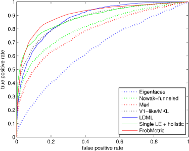
(a)

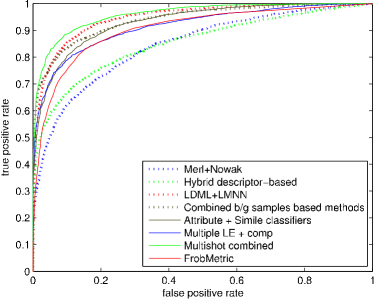
(b)

Figure 2: (a) ROC Curves that use a single descriptor and a single classifier. (b) ROC curves that use hybrid descriptors or single classifiers and FrobMetric’s curve. Each point on a curve is the average over the 10 runs.

Simple recognition systems with a single descriptor Table II shows the performance of FrobMetric’s under varying PCA dimensionality and number of triplets. Increasing the number of training triplets gives a slight improvement in recognition accuracy. The dimension after PCA has more impact on the final accuracy for this task. We also report the CPU time required.

In Figure 2 we show ROC curves for FrobMetric and related face recognition algorithms. These curves were generated by altering the threshold value across the distributions of match and mismatch similarity scores within M$k$NN. Figure 2 (a) shows methods that use a single descriptor and a single classifier only. As can be seen, our system using FrobMetric outperforms all others.

Complex recognition systems with one or more descriptors Figure 2 (b) plots the performance of more complicated recognition systems that use hybrid descriptors or combinations of classifiers. See Table III for details.

TABLE III: Test accuracy (%) on LFW datasets. ROC curve labels in Figure 2 are described here with details.

	SIFT or single descriptor + single classifier	multiple descriptors or classifiers
Turk et al. [21]	60.02 (0.79)	-
	‘Eigenfaces’
Nowak et al. [22]	73.93 (0.49)	-
	‘Nowak-funneled’
Huang et al. [23]	70.52 (0.60)	76.18 (0.58)
	‘Merl’	‘Merl+Nowak’
Wolf et al. in 2008[24]	-	78.47 (0.51)
		‘Hybrid descriptor-based’
Wolf et al. in 2009[25]	72.02	86.83 (0.34)
	-	‘Combined b/g samples based methods’
Pinto et al. [26]	79.35 (0.55)	-
	‘V1-like/MKL’
Taigman et al. [27]	83.20 (0.77)	89.50 (0.40)
	-	‘Multishot combined’
Kumar et al. [28]	-	85.29 (1.23)
		‘attribute + simile classifiers’
Cao et al. [29]	81.22 (0.53)	84.45 (0.46)
	‘single LE + holistic’	‘multiple LE + comp’
Guillaumin et al. [19]	83.2 (0.4)	87.5 (0.4)
	‘LDML’	‘LMNN + LDML’
FrobMetric (this work)	84.34 (1.23)	-
	‘FrobMetric’ on SIFT

As stated above, the leading algorithms have used either 1) additional appearance information, 2) multiple scores from multiple descriptors, or 3) complex recognition systems with hybrids of two or more methods. In contrast, our system using FrobMetric employs neither a combination of other methods nor multiple descriptors. That is, our system exploits a very simple recognition pipeline. The method thus reduces the computational costs associated with extracting the descriptors, generating the prior information, training, and computing the recognition scores.

With such a simple metric learning approach, and modest computational cost, it is notable that the method is only slightly outperformed by state-of-the-art hybrid systems (test accuracy of $84.34\%\pm 1.23\%$ versus $89.50\%\pm 0.40\%$ on the LFW datasets). We would expect that the accuracy of the FrobMetric approach would improve similarly if more features, such as local binary pattern (LBP) [30] for instance, were used.

The FrobMetric approach shows better classification performance at a lower computational cost than comparable single descriptor methods. Despite this level of performance it is surprisingly simple to implement, in comparison to the state-of-the-art.

IV-A3 Metric learning for action recognition

In this experiment, we compare the performance of the proposed method with that of existing approaches on two action recognition benchmark data sets, KTH [31] and Weizmann [32]. Some examples of the actions are shown in Figure 3. We aim to demonstrate again the advantage of our method in reducing computational overhead while achieving excellent recognition performance.

The KTH dataset in this experiment consists $2,387$ video sequences. They can be categorized into six types of human actions including boxing, hand-clapping, jogging, running, walking and hand-waving. These actions are conducted by $25$ subjects and each action is performed multiple times by a same subject. The length of each video is about four seconds at $25$ fps, and the resolution of each frame is $160\times{120}$. We randomly split all the video sequences based on the subjects into $10$ pairs, each of which contains all the sequences from $16$ subjects for training and those from the remaining $9$ subjects for test. The space-time interest points (STIP) [33] were extracted from each video sequence and the the corresponding descriptors calculated. The descriptors extracted from all training sequences were clustered into $4,000$ clusters using $k$-means, with the cluster centers used to form a visual codebook. Accordingly, each video sequence is characterized by a $4000$-dimensional histogram indicating the occurrence of each visual word in this sequence. To achieve a compact and discriminative representation, a recently proposed visual word merging algorithm, called AIB [34], is applied to merge the histogram bins to reduce the dimensionality. Subsequently each video sequence is represented by a $500$-dimensional histogram.

The Weizmann data set contains temporal segmentations of video sequences into ten types of human actions including running, walking, skipping, jumping-jack, jumping-forward-on-two-legs, jumping-in-place-on-two-legs, galloping-sideways, waving-two-hands, waving-one-hand, and bending. The actions are performed by $9$ actors. The action video sequences are represented by space-time shape features such as space-time “saliency”, degree of “plateness”, and degree of “stickness” which compute the degree of location and orientation movement in space-time domain by a Poisson equation [35]. This leads to a $286$-dimensional feature vector for each action video sequence, which is as in [35]. In this experiment, $70\%$ sequences are used for training and the remaining $30\%$ for testing.

The experimental results are shown in Table IV. The first part of the table shows the experimental setting and the second compares the results of various metric learning methods. On the KTH data set, the proposed method, FrobMetric, performs almost as well as BoostMetric with an error rate of $7.03\pm{1.46}\%$, and outperforms all others. In doing so FrobMetric requires only $289.58$ seconds to complete the metric learning, which is approximately one quarter of the time required by the fastest competing method (which has more than double the error rate). On the Weizmann data set, the error rate of FrobMetric is $0.59\pm{0.20}\%$, which is the second-best among all the compared methods. It is slightly higher than (but still comparable to) the lowest one $0.30\pm{0.09}\%$ obtained by LMNN. However, in terms of computational efficiency, FrobMetric requres approximately one eighth of the time used by LMNN, and is the fastest of the methods compared. These results demonstrate the computational efficiency and the excellent classification performance of the proposed method in action recognition.

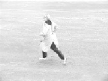
boxing handclapping handwaving jogging running walking

Figure 3: Examples of the actions from the KTH action dataset [31].

TABLE IV: Comparison of FrobMetric and other metric learning methods on action recognition datasets with $3$-NN (Standard deviation is reported for the datasets having multiple runs).

		KTH	Weizmann
# samples		2,387	5,594
# triplets		13,761	35,280
dimension		500	286
# training		1,529	3,920
test		858	1,674
# classes		6	10
# runs		10	10
Error Rates $\%$	Euclidean	10.55 (2.46)	1.14 (0.19)
	RCA	21.05 (3.86)	3.21 (0.66)
	LMNN	15.72 (2.57)	0.30 (0.09)
	ITML	27.67 (1.47)	1.06 (0.16)
	BoostMetric	7.05 (1.42)	0.85 (0.31)
	FrobMetric	7.03 (1.46)	0.59 (0.20)
Comp. Time	LMNN	1023.89s	1343.25s
	ITML	1004.94s	368.68s
	BoostMetric	4048.67	1139.02s
	FrobMetric	289.58s	169.30s

IV-B Maximum variance unfolding

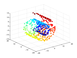
original data

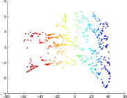
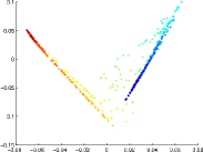
(a)	(b)

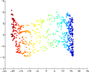
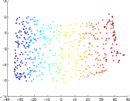
(c)	(d)

Figure 4: Embedding results of different methods on the 3D swiss-roll dataset, with the neighborhood size $k=6$ for all, and $\sigma=10^{5}$ for our method. (a) Isomap, (b) LLE, (c) Our method, (d) MVU.

In this section, we run MVU experiments on a few datasets and compare with other embedding methods. Figure 4 shows the embedding results for several different methods, namely, isometric mapping (Isomap) [36], locally linear embedding (LLE) [37] and MVU [11] on the 3D swiss-roll with 500 points. We use $k=6$ nearest neighbors to construct the local distance constraints and set $\sigma=10^{5}$.

We have also applied our method to the teapot and face image datasets from [11]. The teapot set contains $200$ images obtained by rotating a teapot through $360^{\circ}$. Each image is of $101\times 76$ pixels. Figure 5 shows the two dimensional embedding results of our method and MVU. As can be seen, both methods preserve the order of teapot images corresponding to the angles from which the images were taken, and produce plausible embeddings. But in terms of running time, our algorithm is more than an order of magnitude faster than MVU, requiring only $4$ seconds to run using $k=6$ and $\sigma=10^{10}$, while MVU required $85$ seconds.

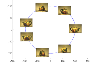
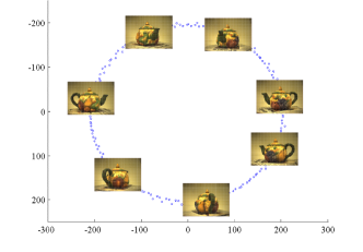
Figure 5: Embedding results of our method and MVU on the teapot dataset; (top) our results with $\sigma=10^{10}$ and (bottom) MVU’s results.

Figure 6 shows a two-dimensional embedding of the images from the face dataset. The set contains $1,965$ images (at $28\times 20$ pixels) of the same individual from different views and with differing expressions. The proposed method required $131$ seconds to solve this metric using $k=5$ nearest neighbors whereas the original MVU needed $4732$ seconds.

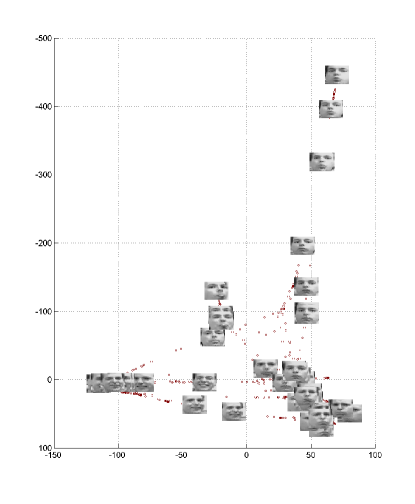
Figure 6: 2D embedding of face data by our approach.

IV-B1 Quantitative Assessment

To better illustrate the effectiveness of our method, here we provide a quantitative evaluation of the embeddings generated for the 3D swiss-roll and teapot datasets. Specifically, we adopt two quality mapping indexes, the unweighted $Q_{nx}$ and $B_{nx}$ [38], to measure the K-ary neighborhood preservation between the high and low dimensional spaces. $Q_{nx}$ represents the proportion of points that remain inside the K-neighborhood after projection, and thus larger $Q_{nx}$ indicates better neighborhood preservation. $B_{nx}$ is defined as the difference in the fractions of mild K-extrusions and mild K-intrusions. It indicates the “behavior” of a dimensionality reduction method, namely, whether it tends to produce an “intrusive” ($B_{nx}(K)>0$) or “extrusive” ($B_{nx}(K)<0$) embedding. Intrusive embedding tends to crush the manifold, which means faraway points can become neighbors after embedding, while extrusive one tends to tear the manifold, meaning some close neighbors can be embedded faraway from each other. In an ideal projection, $B_{nx}$ should be zero. See [38] for more details.

The comparison of LLE, Isomap, MVU and our proposed method on the teapot (with $\sigma=10^{10}$) and the swiss roll ($\sigma=10^{5}$) datasets are shown in Figure 7 and Figure 8. As can be seen from Figure 7 and Figure 8 (a), the proposed FrobMetric method performs on par with MVU, while better than both Isomap and LLE in terms of neighborhood preservation. Note that all methods tend to tear the manifold as $B_{nx}(K)$ is below zero in all cases.

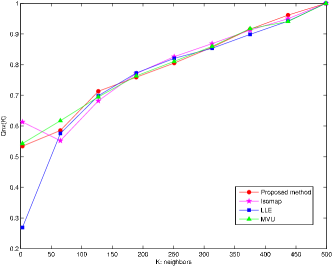
(a)

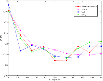
(b)

Figure 7: Quality assessment of neighborhood preservation of different algorithms on 3D swiss roll; (a) $Q_{nx}(K)$;(b) $B_{nx}(K)$.

(a)

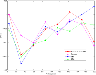
(b)

Figure 8: Quality assessment of neighborhood preservation of different algorithms on teapot dataset; (a) $Q_{nx}(K)$; (b) $B_{nx}(K)$.

We have also made quantitative analysis of the proposed algorithm based on Zhang et al. [39]. They proposed several quantitative criteria, specifically, average local standard deviation (ALSTD) and average local extreme deviation (ALED) to measure the global smoothness of a recovered low-dimensional manifold; average local co-directional consistence (ALCD) to estimate the average co-directional consistence of the principle spread direction (PSD) of the data points, and a combined criteria to simultaneously evaluate the global smoothness and co-directional consistence (GSCD).

We give the visual results of swiss-roll dataset based on PSD in Figure 9, in which the longer line at each sample represents the first PSD, and the second line is orthogonal to the first PSD. We also report the ALSTD and ALED, ALCD and GSCD in Table V and Table VI. From the tables we see that MVU performs best on this swiss-roll dataset, while the proposed FrobMetric method ranks the second best. On the teapot dataset, the proposed method performs slightly better than MVU, while worse than both Isomap and LLE. Overall, the proposed method is similar to the original MVU in terms of these embedding quality criteria. However, note that the proposed method is much faster than MVU in all cases.

original data

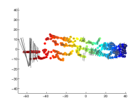
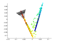
(a)	(b)

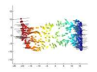
(c)	(d)

Figure 9: Visualization results based on PSD on 3D swiss roll, with the neighborhood size $k=6$ for all, and $\sigma=10^{5}$ for our method; (a)Isomap, (b)LLE, (c) our method, (d) MVU.

TABLE V: ALSTD and ALED results on the 3D swiss roll and teapot datasets

Algorithm	FrobMetric	MVU	Isomap	LLE
ALSTD
Swiss roll	0.113	0.038	0.245	0.328
Teapot	0.377	0.481	0.0611	0.0805
ALED
Swiss roll	0.311	0.102	0.668	0.886
Teapot	1.0	1.28	0.173	0.232

TABLE VI: ALCD and GSCD results on the 3D swiss roll and teapot datasets

Algorithm	FrobMetric	MVU	Isomap	LLE
ALCD
Swiss roll	0.983	0.964	0.969	0.994
Teapot	0.995	0.942	0.997	0.995
GSCD
Swiss roll	0.1163	0.0404	0.2572	0.3317
Teapot	0.3792	0.5105	0.0613	0.0808

To show the efficiency of our approach, in Figure 10 we have compared the computational time between the original MVU implementation and the proposed method, by varying the number of data samples, which determines the number of variables in MVU. Note that the original MVU implementation uses CSDP [40], which is an interior-point based Newton algorithm. We use the 3D “swiss-roll” data here.

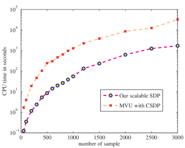
Figure 10: Comparison of computational time on 3D Swiss roll dataset between MVU and our fast approach. Our algorithm uses $\sigma=10^{2}$. Our algorithm is about $15$ times faster. Note that the $y$-axis is in log-scale.

V Conclusion

We have presented an efficient and scalable semidefinite metric learning algorithm. Our algorithm is simple to implement and much more scalable than most SDP solvers. The key observation is that, instead of solving the original primal problem, we solve the Lagrange dual problem by exploiting its special structure. Experiments on UCI benchmark data sets as well as the unconstrained face recognition task show its efficiency and efficacy. We have also extended it to solve more general Frobenius norm regularized SDPs.

References

- [1] K. Q. Weinberger, J. Blitzer, and L. K. Saul, “Distance metric learning for large margin nearest neighbor classification,” J. Mach. Learn. Res., vol. 10, pp. 207–244, 2009.
- [2] C. Shen, J. Kim, and L. Wang, “Scalable large-margin Mahalanobis distance metric learning,” IEEE Trans. Neural Networks, vol. 21, no. 9, pp. 1524–1530, 2010.
- [3] E. Xing, A. Ng, M. Jordan, and S. Russell, “Distance metric learning, with application to clustering with side-information,” in Proc. Adv. Neural Inf. Process. Syst. 2002, pp. 505–512, MIT Press.
- [4] C. Domeniconi, D. Gunopulos, and J. Peng, “Large margin nearest neighbor classifiers,” IEEE Trans. Neural Networks, vol. 16, no. 4, pp. 899–909, 2005.
- [5] J. Goldberger, S. Roweis, G. Hinton, and R. Salakhutdinov, “Neighbourhood component analysis,” in Proc. Adv. Neural Inf. Process. Syst. 2004, pp. 513–520, MIT Press.
- [6] N. Shental, T. Hertz, D. Weinshall, and M. Pavel, “Adjustment learning and relevant component analysis,” in Proc. Euro. Conf. Comp. Vis., London, UK, 2002, vol. 4, pp. 776–792, Springer-Verlag.
- [7] J. V. Davis, B. Kulis, P. Jain, S. Sra, and I. S. Dhillon, “Information-theoretic metric learning,” in Proc. Int. Conf. Mach. Learn., Corvalis, Oregon, 2007, pp. 209–216, ACM Press.
- [8] C. Shen, J. Kim, L. Wang, and A. van den Hengel, “Positive semidefinite metric learning with boosting,” in Proc. Adv. Neural Inf. Process. Syst., 2009, pp. 1651–1659.
- [9] C. Shen, J. Kim, L. Wang, and A. van den Hengel, “Positive semidefinite metric learning using boosting-like algorithms,” J. Mach. Learn. Res., vol. 13, pp. 1007−1036, 2012.
- [10] A. Demiriz, K. P. Bennett, and J. Shawe-Taylor, “Linear programming boosting via column generation,” Mach. Learn., vol. 46, no. 1-3, pp. 225–254, March 2002.
- [11] K. Q. Weinberger and L. K. Saul, “Unsupervised learning of image manifolds by semidefinite programming,” Int. J. Comp. Vis., vol. 70, no. 1, pp. 77–90, 2005.
- [12] S. Boyd and L. Xiao, “Least-squares covariance matrix adjustment,” SIAM J. Matrix Analysis & Applications, vol. 27, no. 2, pp. 532–546, 2005.
- [13] C. Shen, J. Kim, and L. Wang, “A scalable dual approach to semidefinite metric learning,” in Proc. IEEE Conf. Comp. Vis. Pattern Recogn., Colorado Springs, USA, 2011, pp. 2601–2608.
- [14] S. Boyd and L. Vandenberghe, Convex Optimization, Cambridge University Press, 2004.
- [15] J. Borwein and A. Lewis, Convex Analysis and Nonlinear Optimization, Springer-Verlag, New York, 2000.
- [16] D. C. Liu and J. Nocedal, “On the limited memory BFGS method for large scale optimization,” Math. Program.: Series A and B, vol. 45, no. 3, pp. 503–528, 1989.
- [17] C.-C. Chang and C.-J. Lin, “LIBSVM: A library for support vector machines,” ACM Trans. Intelligent Systems & Technology, vol. 2, no. 3, pp. 1–27, 2011.
- [18] G. B. Huang, M. Ramesh, T. Berg, and E. Learned-Miller, “Labeled faces in the wild: A database for studying face recognition in unconstrained environments,” Technical Report 07-49, University of Massachusetts, Amherst, October 2007.
- [19] M. Guillaumin, J. Verbeek, and C. Schmid, “Is that you? metric learning approaches for face identification,” in Proc. IEEE Int. Conf. Comp. Vis., 2009, pp. 498–505.
- [20] D. G. Lowe, “Distinctive image features from scale-invariant keypoints,” Int. J. Comp. Vis., vol. 60, no. 2, pp. 91–110, 2004.
- [21] M. A. Turk and A. P. Pentland, “Face recognition using Eigenfaces,” in Proc. IEEE Conf. Comp. Vis. Pattern Recogn., 1991, pp. 586–591.
- [22] E. Nowak and F. Jurie, “Learning visual similarity measures for comparing never seen objects,” in Proc. IEEE Conf. Comp. Vis. Pattern Recogn., 2007, pp. 1–8.
- [23] G. B. Huang, M. J. Jones, and E. Learned-Miller, “LFW results using a combined Nowak plus MERL recognizer,” in Faces in Real-Life Images Workshop, in Euro. Conf. Comp. Vision, 2008.
- [24] L. Wolf, T. Hassner, and Y. Taigman, “Descriptor based methods in the wild,” in Faces in Real-Life Images Workshop, in Euro. Conf. Comp. Vision, 2008.
- [25] L. Wolf, T. Hassner, and Y. Taigman, “Similarity scores based on background samples,” in Proc. Asian Conf. Comp. Vis., 2009, vol. 2, pp. 88–97.
- [26] N. Pinto, J. DiCarlo, and D. Cox, “How far can you get with a modern face recognition test set using only simple features?,” in Proc. IEEE Conf. Comp. Vis. Pattern Recogn., 2009, pp. 2591–2598.
- [27] Y. Taigman, L. Wolf, and T. Hassner, “Multiple one-shots for utilizing class label information,” in Proc. British Mach. Vis. Conf., 2009.
- [28] N. Kumar, A. C. Berg, P. N. Belhumeur, and S. K. Nayar, “Attribute and simile classifiers for face verification,” in Proc. IEEE Int. Conf. Comp. Vis., 2009, pp. 365–372.
- [29] Z. Cao, Q. Yin, X. Tang, and J. Sun, “Face recognition with learning-based descriptor,” in Proc. IEEE Conf. Comp. Vis. Pattern Recogn., 2010, pp. 2707–2714.
- [30] T. Ahonen, A. Hadid, and M. Pietikainen, “Face Description with Local Binary Patterns: Application to Face Recognition,” IEEE Trans. Pattern Anal. Mach. Intell., vol. 28, pp. 2037–2041, 2006.
- [31] C. Schüldt, I. Laptev, and B. Caputo, “Recognizing human actions: A local SVM approach,” Proc. Int. Conf. Pattern Recogn., vol. 3, pp. 32–36, 2004.
- [32] L. Gorelick, M. Blank, E. Shechtman, M. Irani, and R. Basri, “Actions as space-time shapes,” IEEE Trans. Pattern Anal. Mach. Intell., vol. 29, no. 12, pp. 2247–2253, 2007.
- [33] I. Laptev, M. Marszalek, C. Schmid, and B. Rozenfeld, “Learning realistic human actions from movies,” in Proc. IEEE Conf. Comp. Vis. Pattern Recogn., 2008, pp. 1–8.
- [34] B. Fulkerson, A. Vedaldi, and S. Soatto, “Localizing objects with smart dictionaries,” in Proc. Euro. Conf. Comp. Vis. 2008, pp. 179–192, Springer-Verlag.
- [35] D. Tran and A. Sorokin, “Human activity recognition with metric learning,” in Proc. Euro. Conf. Comp. Vis. 2008, pp. 548–561, Springer-Verlag.
- [36] J. B. Tenenbaum, V. de Silva, and J. C. Langford, “A global geometric framework for nonlinear dimensionality reduction,” Science, vol. 290, pp. 2319–2323, 2000.
- [37] S. Roweis and L. Saul, “Nonlinear dimensionality reduction by locally linear embedding,” Science, vol. 290, pp. 2323–2326, 2000.
- [38] J. Lee and M. Verleysen, “Quality assessment of nonlinear dimensionality reduction based on k-ary neighborhoods,” JMLR Proc. New challenges for feature selection in data mining and knowledge discovery, vol. 4, pp. 21–35, 2008.
- [39] J. Zhang, Q. Wang, L. He, and Z.-H. Zhou, “Quantitative analysis of nonlinear embedding,” IEEE Trans. Neural Networks, vol. 22, no. 12, pp. 1987–1998, 2011.
- [40] B. Borchers, “CSDP, a C library for semidefinite programming,” Optim. Methods and Softw., vol. 11, no. 1, pp. 613–623, 1999.