Improved Dual Decomposition Based Optimization for DSL Dynamic Spectrum Management

Abstract

Dynamic spectrum management (DSM) has been recognized as a key technology to significantly improve the performance of digital subscriber line (DSL) broadband access networks. The basic concept of DSM is to coordinate transmission over multiple DSL lines so as to mitigate the impact of crosstalk interference amongst them. Many algorithms have been proposed to tackle the nonconvex optimization problems appearing in DSM, almost all of them relying on a standard subgradient based dual decomposition approach. In practice however, this approach is often found to lead to extremely slow convergence or even no convergence at all, one of the reasons being the very difficult tuning of the stepsize parameters. In this paper we propose a novel improved dual decomposition approach inspired by recent advances in mathematical programming. It uses a smoothing technique for the Lagrangian combined with an optimal gradient based scheme for updating the Lagrange multipliers. The stepsize parameters are furthermore selected optimally removing the need for a tuning strategy. With this approach we show how the convergence of current state-of-the-art DSM algorithms based on iterative convex approximations (SCALE, CA-DSB) can be improved by one order of magnitude. Furthermore we apply the improved dual decomposition approach to other DSM algorithms (OSB, ISB, ASB, (MS)-DSB, MIW) and propose further improvements to obtain fast and robust DSM algorithms. Finally, we demonstrate the effectiveness of the improved dual decomposition approach for a number of realistic multi-user DSL scenarios.

EDICS: SPC-TDLS Telephone networks and digital subscriber loops, SPC-MULT Multi-carrier, OFDM, and DMT communications, MSP-APPL Applications of MIMO communications and signal processing

I Introduction

Digital subscriber line (DSL) technology refers to a family of technologies that provide digital broadband access over the local telephone network. It is currently the dominating broadband access technology with 66% of all broadband access subscribers worldwide using DSL to access the Internet [1]. The major obstacle for further performance improvement in modern DSL networks is the so-called crosstalk, i.e. the electromagnetic interference amongst different lines in the same cable bundle. Different lines (i.e. users) indeed interfere with each other, leading to a very challenging interference environment where proper management of the resources is required to prevent a huge performance degradation.

Dynamic spectrum management (DSM) has been recognized as a key technology to significantly improve the performance of DSL broadband access networks [2]. The basic concept of DSM is to coordinate transmission over multiple DSL lines so as to mitigate the impact of crosstalk interference amongst them. There are two types of coordination referred to as spectrum level and signal level coordination. Here, we will focus on spectrum level coordination, also referred to as spectrum management, spectrum balancing or multi-carrier power control. Spectrum management aims to allocate transmit spectra, i.e. transmit powers over all available frequencies (tones), to the different users so as to achieve some design objective. This generally corresponds to an optimization problem, where typically a weighted sum of user data rates is maximized subject to power constraints [3, 4, 5], which will be referred to as “constrained weighted rate sum maximization (cWRS)”. Recently this has been extended to other design objectives as well, such as power driven designs (green DSL[6],[7], [8]) and other utility driven designs [9, 10]. As shown in [6], the key component to these designs is an efficient solution for the cWRS problem. Therefore we will mainly focus on this problem and aim to find a robust and efficient solution for it.

The cWRS problem is known to be an NP-hard, separable nonconvex optimization problem, that can have many locally optimal solutions [9][11]. Even for moderately sized problems (with 5-20 users and 200-4000 tones), finding the globally optimal solution is computationally prohibitive. In [3] and [4] the authors proposed to use a dual decomposition approach with a standard subgradient based updating of the Lagrange multipliers. Many DSM algorithms [3, 5, 12, 13, 11, 14, 15, 16, 17, 18] have been proposed recently, almost all of them using this standard subgradient based dual decomposition approach. In practice, however, this approach is often found to lead to extremely slow convergence or even no convergence at all, especially so for large DSL scenarios with large crosstalk. One of the reasons is the very difficult tuning of the stepsize parameters so as to guarantee fast convergence.

In this paper we propose a novel improved dual decomposition approach inspired by recent advances in mathematical programming, more specifically the proximal center based decomposition method recently proposed in [19]. This method uses a smoothing technique for the Lagrangian that preserves separability of the problem, as recently proposed in [20]. The corresponding stepsize is determined in an optimal way and so straightforwardly tuned. The method is originally designed for separable convex problems, whereas DSM optimization problems are highly nonconvex. In this paper we extend the proximal center based decomposition method to an improved dual decomposition approach for application in the context of DSM. With this approach, we show how the convergence of current state-of-the-art DSM algorithms based on iterative convex approximations (SCALE[14], CA-DSB[11]) can be improved by one order of magnitude. Furthermore we apply the improved dual decomposition approach to other DSM algorithms (OSB[3], PBnB[12], ISB[13], ASB[16], (MS-)DSB[11], MIW[15], BB-OSB[5]), again leading to much faster converging DSM algorithms. Then we demonstrate an important pitfall of applying dual decomposition to nonconvex DSM problems and propose an effective solution for this that further improves the robustness of current DSM algorithms. Finally we demonstrate the effectiveness of the improved dual decomposition approach for a number of realistic multi-user DSL scenarios.

This paper is organized as follows. In Section II, the system model is introduced for the DSL multi-user environment. In Section III, the basic cWRS problem is described and existing DSM algorithms for this problem are reviewed, all of them relying on a subgradient based dual decomposition approach. In Section IV-A an improved dual decomposition approach is proposed for DSM algorithms based on iterative convex approximations. The improved dual decomposition approach is furthermore applied to other DSM algorithms in Section IV-B. In Section V, the problem of obtaining a primal solution from the dual solution is described and an effective solution for it is proposed. Finally in Section VI, simulation results are shown.

II System Model

We consider a system consisting of $\mathcal{N}=\{1,\ldots,N\}$ interfering DSL users (i.e., lines, modems) with standard synchronous discrete multi-tone (DMT) modulation with $\mathcal{K}=\{1,\ldots,K\}$ tones (i.e., frequencies or carriers). The transmission can be modeled independently on each tone $k$ by

$$\mathbf{y}_{k}=\mathbf{H}_{k}\mathbf{x}_{k}+\mathbf{z}_{k}.$$

The vector $\mathbf{x}_{k}=[x^{1}_{k},\ldots,x^{N}_{k}]^{T}$ contains the transmitted signals on tone $k$, where $x_{k}^{n}$ refers to the signal transmitted by user $n$ on tone $k$. Vectors $\mathbf{z}_{k}$ and $\mathbf{y}_{k}$ have similar structures; $\mathbf{z}_{k}$ refers to the additive noise on tone $k$, containing thermal noise, alien crosstalk, radio frequency interference (RFI), etc, and $\mathbf{y}_{k}$ refers to the received signals on tone $k$. $\mathbf{H}_{k}$ is an $N\times N$ channel matrix with $[\mathbf{H}_{k}]_{n,m}=h^{n,m}_{k}$ referring to the channel gain from transmitter $m$ to receiver $n$ on tone $k$. The diagonal elements are the direct channels and the off-diagonal elements are the crosstalk channels.

The transmit power of user $n$ on tone $k$, also referred to as transmit power spectral density, is denoted as $s^{n}_{k}\triangleq\Delta_{f}E\{|x^{n}_{k}|^{2}\}$, where $\Delta_{f}$ refers to the tone spacing. The vector $\mathbf{s}_{k}\triangleq\{s_{k}^{n},n\in\mathcal{N}\}$ denotes the transmit powers of all users on tone $k$. The vector $\mathbf{s}^{n}\triangleq\{s_{k}^{n},k\in\mathcal{K}\}$ denotes the transmit powers of user $n$ on all tones. The received noise power by user $n$ on tone $k$, also referred to as noise spectral density, is denoted as $\sigma^{n}_{k}\triangleq\Delta_{f}E\{|z^{n}_{k}|^{2}\}$.

Note that we assume no signal coordination at the transmitters and at the receivers, and that the interference is treated as additive white Gaussian noise. Under this standard assumption the bit loading for user $n$ on tone $k$, given the transmit spectra $\mathbf{s}_{k}$ of all users on tone $k$, is

$$b^{n}_{k}\triangleq b^{n}_{k}(\mathbf{s}_{k})\triangleq\mathrm{log}_{2}\Bigg{(}1+\frac{1}{\Gamma}\frac{|h^{n,n}_{k}|^{2}s^{n}_{k}}{{\displaystyle\sum_{m\neq n}}|h^{n,m}_{k}|^{2}s^{m}_{k}+\sigma^{n}_{k}}\Bigg{)}~{}\mathrm{bits/Hz},$$ (1)

where $\Gamma$ denotes the SNR-gap to capacity, which is a function of the desired BER, the coding gain and noise margin [21]. The DMT symbol rate is denoted as $f_{s}$. The achievable total data rate for user $n$ and the total power used by user $n$ are equal to, respectively:

$$\begin{array}[]{l}R^{n}\triangleq f_{s}{\displaystyle\sum_{k\in\mathcal{K}}}b^{n}_{k},\\ P^{n}\triangleq{\displaystyle\sum_{k\in\mathcal{K}}}s^{n}_{k}.\end{array}$$ (2)

III Dynamic spectrum management

III-A Dynamic spectrum management problem

The basic goal of DSM through spectrum level coordination is to allocate the transmit powers dynamically in response to physical channel conditions (channel gains and noise) so as to pursue certain design objectives and/or satisfy certain constraints. The constraints are mostly per-user total power constraints and so-called spectral mask constraints, i.e.

$$\begin{array}[]{l}P^{n}\leq P^{n,\mathrm{tot}}\qquad\qquad n\in\mathcal{N}\qquad\qquad\ \ \ (\mathrm{total~{}power~{}constraints})\\ 0\leq s_{k}^{n}\leq s_{k}^{n,\mathrm{mask}}\qquad n\in\mathcal{N},k\in\mathcal{K}\qquad(\mathrm{spectral~{}mask~{}constraints})\end{array}$$ (3)

where $P^{n,\mathrm{tot}}$ refers to the total available power budget for user $n$ and $s_{k}^{n,\mathrm{mask}}$ refers to the spectral mask constraint for user $n$ on tone $k$. The user total power constraints can also be written in vector notation as $\mathbf{P}\leq\mathbf{P}^{\mathrm{tot}}$, where $\mathbf{P}=[P^{1},\ldots,P^{N}]^{T}$ and $\mathbf{P}^{\mathrm{tot}}=[P^{1,\mathrm{tot}},\ldots,P^{N,\mathrm{tot}}]^{T}$, and where ’$\leq$’ denotes a component-wise inequality.

The set of all possible data rate allocations that satisfy the constraints (3) can be characterized by the achievable rate region $\mathcal{R}$:

$$\mathcal{R}=\Big{\{}(R^{n}:n\in\mathcal{N})|R^{n}=f_{s}\sum_{k\in K}b^{n}_{k}(\mathbf{s}_{k}),\mathrm{~{}s.t.~{}(\ref{eq:DSLstandard})}\Big{\}}.$$

A typical design objective is to achieve some Pareto optimal allocation of the data rates $R^{n}$ [18, 3, 13, 22, 12, 5, 16, 23, 14, 15, 11]. This results in the following typical DSM optimization problem, which will be referred as the constrained weighted rate sum maximization (cWRS) formulation, where $w_{n}$ is the weight given to user $n$:

$$\begin{array}[]{cl}{\displaystyle\max_{\{\mathbf{s}^{n},n\in\mathcal{N}\}}}&{\displaystyle\sum_{n\in\mathcal{N}}}w_{n}R^{n}\\ \mathrm{s.t.}&P^{n}\leq P^{n,\mathrm{tot}},\quad\qquad n\in\mathcal{N},\qquad\qquad\qquad(\mathrm{cWRS})\\ &0\leq s^{n}_{k}\leq s^{n,\mathrm{mask}}_{k},\quad n\in\mathcal{N},k\in\mathcal{K}.\end{array}$$ (4)

However, many other DSM formulations are possible. We refer to [6] containing a collection of other relevant DSM formulations. As shown in [6], the key component to tackling these is an efficient solution for cWRS problem (4). Therefore we will focus on this problem and aim to find a robust and efficient solution for it.

III-B Dynamic spectrum management algorithms

cWRS problem (4) is an NP-hard separable nonconvex optimization problem [9]. The number of optimization variables is equal to $KN$, where the number of users $N$ ranges between 2-100 and the number of tones $K$ can go up to 4000. Depending on the specific values of the channel and noise parameters, there can be many locally optimal solutions, that can differ significantly in value, as shown in [11]. In [4] the authors show that strong duality holds for the continuous (frequency range) formulation, and in [9] the authors prove asymptotic strong duality for the discrete (frequency range) formulation, i.e. the duality gap goes to zero as $K\rightarrow\infty$. These results suggest that a Lagrange dual decomposition approach is a viable way to reach approximate optimality for the discrete formulation (4), if the frequency range is finely discretized, as it is indeed the case in practical DSL scenarios where $K$ is large [4]. Many dual decomposition based DSM algorithms [3, 5, 12, 13, 11, 14, 15, 16, 18] have been proposed for solving (4), almost all of them using a standard subgradient based updating of the Lagrange multipliers.

The dual problem formulation of (4) consists of two subproblems, namely a master problem

$$\begin{array}[]{cl}{\displaystyle\min_{\mathbf{\lambda}}}&g(\mathbf{\lambda})\\ \mathrm{s.t.}&\mathbf{\lambda}\geq 0\end{array}$$ (5)

where $\mathbf{\lambda}=[\lambda_{1},\ldots,\lambda_{N}]^{T}$, and a slave problem defined by the dual function $g(\mathbf{\lambda})$:

$$\begin{array}[]{l}g(\mathbf{\lambda})=\mathcal{L}(\mathbf{\lambda},\mathbf{s}_{k},k\in\mathcal{K})=\Bigg{\{}\begin{array}[]{cl}{\displaystyle\max_{\{\mathbf{s}_{k},k\in\mathcal{K}\}}}&{\displaystyle\sum_{n\in\mathcal{N}}}w_{n}R^{n}-{\displaystyle\sum_{n\in\mathcal{N}}}\lambda_{n}(P^{n}-P^{n,\mathrm{tot}})\\ \mathrm{s.t.}&0\leq s_{k}^{n}\leq s_{k}^{n,\mathrm{mask}},\qquad n\in\mathcal{N},k\in\mathcal{K},\end{array}\end{array}$$ (6)

where $\mathcal{L}(\mathbf{\lambda},\mathbf{s}_{k},k\in\mathcal{K})$ is the Lagrangian. This can be reformulated as:

$$\begin{array}[]{l}g(\mathbf{\lambda})=\Bigg{\{}\begin{array}[]{cl}{\displaystyle\max_{\{\mathbf{s}_{k},k\in\mathcal{K}\}}}&{\displaystyle\sum_{k\in\mathcal{K}}}\Big{\{}f_{s}b_{k}(\mathbf{s_{k}})-{\displaystyle\sum_{n\in\mathcal{N}}}\lambda_{n}s_{k}^{n}\Big{\}}+{\displaystyle\sum_{n\in\mathcal{N}}}\lambda_{n}P^{n,\mathrm{tot}}\\ \mathrm{s.t.}&0\leq s_{k}^{n}\leq s_{k}^{n,\mathrm{mask}},\qquad n\in\mathcal{N},k\in\mathcal{K}\end{array}\\ \mathrm{with~{}~{}}b_{k}(\mathbf{s}_{k})={\displaystyle\sum_{n\in\mathcal{N}}}w_{n}b_{k}^{n}(\mathbf{s}_{k})\end{array}$$ (7)

The slave optimization problem (7) can then be decomposed into $K$ independent nonconvex subproblems (dual decomposition):

$$\begin{array}[]{l}g(\mathbf{\lambda})={\displaystyle\sum_{k\in K}}g_{k}(\mathbf{\lambda})\\ \mathrm{with~{}}g_{k}(\mathbf{\lambda})=\Bigg{\{}\begin{array}[]{cl}{\displaystyle\max_{\mathbf{s}_{k}}}&f_{s}b_{k}(\mathbf{s}_{k})-{\displaystyle\sum_{n\in\mathcal{N}}}\lambda_{n}s_{k}^{n}+{\displaystyle\sum_{n\in\mathcal{N}}}\lambda_{n}P^{n,\mathrm{tot}}/K\\ \mathrm{s.t.}&0\leq s_{k}^{n}\leq s_{k}^{n,\mathrm{mask}},\quad n\in\mathcal{N}\end{array}\\ \end{array}\\$$ (8)

The master problem (5), also called the dual problem, is a convex optimization problem. Its objective function, i.e. the dual function $g(\mathbf{\lambda})$, is however non-differentiable. The reason for this non-differentiability is that the underlying slave optimization problem (6) can have multiple globally optimal solutions for some values of the Lagrange multipliers $\mathbf{\lambda}$. In [4][3] a subgradient approach is proposed for this dual master problem, where the subgradient is defined as,

$$dg(\mathbf{\lambda})\triangleq\sum_{k\in\mathcal{K}}\mathbf{s}_{k}(\mathbf{\lambda})-\mathbf{P}^{\mathrm{tot}}$$ (9)

with $\mathbf{s}_{k}(\mathbf{\lambda})$ referring to the optimal solution of (8) for given Lagrange multipliers $\mathbf{\lambda}$, also called dual variables, and the corresponding subgradient update is:

$$\mathbf{\lambda}=\Big{[}\mathbf{\lambda}+\delta(\sum_{k\in\mathcal{K}}\mathbf{s}_{k}(\mathbf{\lambda})-\mathbf{P}^{\mathrm{tot}})\Big{]}^{+},$$ (10)

where $[\mathbf{x}]^{+}$ denotes the projection of $\mathbf{x}\in\mathcal{R}^{N}$ onto $\mathcal{R}^{N}_{+}$, and where the stepsize $\delta$ can be chosen using different procedures [4, 5], e.g. $\delta=q/i$ where $q$ is the initial stepsize and $i$ is the iteration counter. By iteratively applying (10) and (8), convergence to an optimal solution of (5) can be achieved, i.e. $\mathbf{\lambda}\rightarrow\mathbf{\lambda}^{*}$, for which the complementary conditions, $\lambda_{n}(\sum_{k\in\mathcal{K}}\mathbf{s}^{n}_{k}(\mathbf{\lambda})-\mathbf{P}^{n,\mathrm{tot}})=0,\ n\in\mathcal{N}$, are satisfied when strong duality “holds” ($K\rightarrow\infty$). This general standard dual decomposition approach is visualized in Figure 1.

Note that the per-tone subproblems (8) are nonconvex optimization problems. Many existing DSM algorithms differ only in the way these subproblems are solved, where strategies are proposed such as exhaustive discrete search (OSB)[3], branch and bound search (PBnB[12], BB-OSB[5]), coordinate descent discrete search (ISB)[13][22], solving the KKT system (DSB[11], MIW[15], MS-DSB[11]), and heuristic approximation (ASB[16], ASB2[11]).

Figure 1: General structure of subgradient based dual decomposition approach for DSM

An alternative approach is based on iterative convex approximations such as in SCALE[14] and CA-DSB[11]. This approach basically consists of iteratively executing the following two steps: (i) approximating the nonconvex cWRS problem (4) by a separable convex optimization problem $F_{\mathrm{cvx}}$, and (ii) solving this convex approximation by using a subgradient based dual decomposition approach. Note that under some conditions on the approximation, described in [24], iteratively executing these steps results in asymptotic convergence to a locally optimal solution of cWRS (4). The convex approximations used by CA-DSB and SCALE both satisfy these conditions. This approach is visualized in Figure 2, where $F_{k,\mathrm{cvx}}$ refers to the per-tone convex problem obtained from the convex approximation $F_{\mathrm{cvx}}$. We emphasize that these DSM algorithms also use a subgradient based dual decomposition approach to solve a convex optimization problem in each iteration. This step requires the major part of the computational cost.

Figure 2: Structure of iterative convex approximation approach for DSM

IV Improved dual decomposition

In practice, the standard subgradient based dual decomposition approach is often found to lead to extremely slow convergence or even no convergence at all, especially so for large DSL scenarios (6-20 users) with large crosstalk (VDSL(2)). This is because of different reasons: (i) subgradient methods are generally known not to be efficient, i.e. showing worst case convergence of order $\mathcal{O}(\frac{1}{\epsilon^{2}})$ with $\epsilon$ referring to the required accuracy of the approximation of the optimum [20], (ii) the stepsize used by subgradient methods is quite difficult to tune in order to guarantee fast convergence, (iii) the nonconvex nature of the problem implies that special care should be taken in obtaining the optimal primal variables from the optimal dual variables.

For separable convex problems, i.e. with a separable convex objective function but with convex coupling constraints, several alternative dual decomposition approaches have been proposed such as the alternating direction method [25], proximal method of multipliers [26], partial inverse method [27], etc. Here, we focus on a recently proposed dual decomposition approach in [19], referred to as the proximal center based decomposition method. This method shows interesting properties, namely it preserves separability of the problem, it uses an optimal gradient based scheme, and it uses an optimal stepsize which leads to straightforward tuning. In this section we extend this method to an improved dual decomposition approach for solving cWRS (4). This approach will be used first in Section IV-A to improve the convergence of DSM algorithms using iterative convex approximations (SCALE, CA-DSB) with one order of magnitude. In Section IV-B this will be extended to other DSM algorithms such as OSB, ISB, PBnB, BB-OSB, ASB, (MS-)DSB, MIW, etc. We will refer to these DSM algorithms that are not based on iterative convex approximations as “direct DSM algorithms”.

IV-A An improved dual decomposition approach for iterative convex approximation based DSM algorithms

Two state-of-the-art DSM algorithms that are based on iterative convex approximations are SCALE and CA-DSB. These basically consist of two steps as explained in Section III-B, which are iteratively executed. In this section we will propose an improved dual decomposition approach for solving the convex optimization problem in the second step. We will elaborate this for CA-DSB and explain how its convergence speed is improved by one order of magnitude, i.e. from $\mathcal{O}(\frac{1}{\epsilon^{2}})$ to $\mathcal{O}(\frac{1}{\epsilon})$. The improved dual decomposition approach can similarly be applied to the SCALE algorithm to obtain a similar speed up, but requires more complicated notation because of the inherent exponential transformation of variables.

For CA-DSB, the convex approximation in each iteration is obtained by reformulating the objective of cWRS, as a sum of a concave part and a convex part, and then approximating the convex part by a first order Taylor expansion. The resulting convex approximation, its dual formulation, dual function, and Lagrangian are given in (11), (12), (13), and (14), respectively.

$$f^{*}_{\mathrm{cvx}}=\big{\{}{\displaystyle\max_{\{\mathbf{s}_{k}\in\mathcal{S}_{k},k\in\mathcal{K}\}}}{\displaystyle\sum_{k\in\mathcal{K}}}b_{k,\mathrm{cvx}}(\mathbf{s}_{k})\ \ \mathrm{s.t.}{\displaystyle\sum_{k\in\mathcal{K}}}s_{k}^{n}\leq P^{n,\mathrm{tot}},\ n\in\mathcal{N}\big{\}}$$ (11)

$${\displaystyle\min_{\mathbf{\lambda}\geq 0}}\ g_{\mathrm{cvx}}(\mathbf{\lambda})$$ (12)

$$g_{\mathrm{cvx}}(\mathbf{\lambda})={\displaystyle\max_{\{\mathbf{s}_{k}\in\mathcal{S}_{k},k\in\mathcal{K}\}}}\mathcal{L}_{\mathrm{cvx}}(\mathbf{s}_{k},k\in\mathcal{K},\mathbf{\lambda})$$ (13)

$$\mathcal{L}_{\mathrm{cvx}}(\mathbf{s}_{k},k\in\mathcal{K},\mathbf{\lambda})={\displaystyle\sum_{k\in\mathcal{K}}}b_{k,\mathrm{cvx}}(\mathbf{s}_{k})-{\displaystyle\sum_{k\in\mathcal{K}}}\ {\displaystyle\sum_{n\in\mathcal{N}}}\lambda_{n}s_{k}^{n}+{\displaystyle\sum_{n\in\mathcal{N}}}\lambda_{n}P^{n,\mathrm{tot}}$$ (14)

where $\mathcal{S}_{k}=\{\mathbf{s}_{k}\in\mathcal{R}^{n}:0\leq s_{k}^{n}\leq s_{k}^{n,\mathrm{max}},n\in\mathcal{N}\}$ is a compact convex set with $s_{k}^{n,\mathrm{max}}:=\min(s_{k}^{n,\mathrm{mask}},P^{n,\mathrm{tot}})$ and $P^{n,\mathrm{tot}}<\infty$, and where $b_{k,\mathrm{cvx}}(\mathbf{s}_{k})$ is concave and given as:

$$\begin{array}[]{l}b_{k,\mathrm{cvx}}(\mathbf{s}_{k})={\displaystyle\sum_{n\in\mathcal{N}}}w_{n}f_{s}\log_{2}({\displaystyle\sum_{m\in\mathcal{N}}}|\tilde{h}_{k}^{n,m}|^{2}s_{k}^{m}+\Gamma\sigma_{k}^{n})-{\displaystyle\sum_{n\in\mathcal{N}}}w_{n}f_{s}({\displaystyle\sum_{m\neq n}}a_{k}^{m,n}s_{k}^{m}+c_{k}^{n}),\\ \end{array}$$ (15)

with $a_{k}^{n,m},c_{k}^{n},\forall n,m,k$ constant approximation parameters, obtained by a closed-form formula in the approximation step [11], and with

$$\begin{array}[]{l}|\tilde{h}_{k}^{n,m}|^{2}\Bigg{\{}\begin{array}[]{l}=\Gamma|h_{k}^{n,m}|^{2},\qquad n\neq m\\ =|h_{k}^{n,m}|^{2},\qquad n=m.\end{array}\end{array}$$ (16)

The convex problem (11) has a separable structure and so the standard way to solve it is by focusing on the dual problem (12) and using a subgradient update approach for the dual variables. This subgradient based dual decomposition approach is however known [20] to have a convergence speed of order $\mathcal{O}(\frac{1}{\epsilon^{2}})$, where $\epsilon$ is the required accuracy for the approximation of the optimum. In the sequel, it will be shown how the “proximal center based decomposition” method from [19] can be adapted for solving the convex approximation, leading to a scheme with convergence speed of order $\mathcal{O}(\frac{1}{\epsilon})$, i.e. one order of magnitude faster but with the same computational complexity. The basic steps in this result are as follows. First an approximated (smoothed) dual function $\bar{g}_{\mathrm{cvx}}(\mathbf{\lambda})$ is defined that can be chosen to be arbitrarily close to the original dual function $g_{\mathrm{cvx}}(\mathbf{\lambda})$. Then it is proven that this smoothed dual function $\bar{g}_{\mathrm{cvx}}$ is differentiable and has a Lipschitz continuous gradient. Finally an optimal gradient scheme is applied to this smoothed dual function.

We introduce the following functions $d_{k}(\mathbf{s}_{k}),k\in\mathcal{K}$, which are called prox-functions in [19] and are defined as follows:

Definition 1

A prox-function $d_{k}(\mathbf{s}_{k})$ has the following properties:

• $d_{k}(\mathbf{s}_{k})$ is a non-negative continuous and strongly convex function with convexity parameter $\sigma_{\mathcal{S}_{k}}$

• $d_{k}(\mathbf{s}_{k})$ is defined for the compact convex set $\mathcal{S}_{k}$

An example of a valid prox-function is $d_{k}(\mathbf{s}_{k})=\frac{1}{2}\|\mathbf{s}_{k}\|^{2}$, which is also used in our concrete implementations (see Section VI). As many other valid prox-functions exist, and in order not to loose generality, we continue with $d_{k}(\mathbf{s}_{k})$. Since $\mathcal{S}_{k},k\in\mathcal{K},$ are compact and $d_{k}(\mathbf{s}_{k})$ are continuous, we can choose finite and positive constants such that

$$D_{\mathcal{S}_{k}}\geq\max_{\mathbf{s}_{k}\in\mathcal{S}_{k}}d_{k}(\mathbf{s}_{k}),k\in\mathcal{K}.$$ (17)

The prox-functions can be used to smoothen the dual function $g_{\mathrm{cvx}}(\mathbf{\lambda})$ to obtain a smoothed dual function $\bar{g}_{\mathrm{cvx}}(\mathbf{\lambda})$ as follows:

$$\bar{g}_{\mathrm{cvx}}(\mathbf{\lambda})=\max_{\{\mathbf{s}_{k}\in\mathcal{S}_{k},k\in\mathcal{K}\}}\sum_{k\in\mathcal{K}}\Big{\{}b_{k,\mathrm{cvx}}(\mathbf{s}_{k})-\sum_{n\in\mathcal{N}}\lambda_{n}(s_{k}^{n}-P^{n,\mathrm{tot}}/K)-cd_{k}(\mathbf{s}_{k})\Big{\}},$$ (18)

where $c$ is a positive smoothness parameter that will be defined later in this section. By using a sufficiently small value for $c$, the smoothed dual function can be arbitrarily close to original dual function. Note that we can also choose different parameters $c_{k}$ for each prox-term. The generalization is straightforward.

One useful property of the particular choice of prox-functions is that they do not destroy the separability of the objective function in (18), i.e.

$$\bar{g}_{\mathrm{cvx}}(\mathbf{\lambda})=\sum_{k\in\mathcal{K}}\bigg{\{}\max_{\mathbf{s}_{k}\in\mathcal{S}_{k}}b_{k,\mathrm{cvx}}(\mathbf{s}_{k})-\sum_{n\in\mathcal{N}}\lambda_{n}(s_{k}^{n}-P^{n,\mathrm{tot}}/K)-cd_{k}(\mathbf{s}_{k})\bigg{\}}.$$ (19)

Denote by $\bar{\mathbf{s}}_{k,\mathrm{cvx}}(\mathbf{\lambda}),k\in\mathcal{K},$ the optimal solution of the maximization problem in (19). The following theorem describes the properties of the smoothed dual function $\bar{g}_{\mathrm{cvx}}(\mathbf{\lambda})$:

Theorem 1 ([19])

The function $\bar{g}_{\mathrm{cvx}}(\mathbf{\lambda})$ is convex and continuously differentiable at any $\mathbf{\lambda}\in\mathcal{R}^{n}$. Moreover, its gradient $\nabla\bar{g}_{\mathrm{cvx}}(\mathbf{\lambda})=\sum_{k\in\mathcal{K}}\bar{\mathbf{s}}_{k,\mathrm{cvx}}(\mathbf{\lambda})-\mathbf{P}^{\mathrm{tot}}$ is Lipschitz continuous with Lipschitz constant $L_{c}=\sum_{k\in\mathcal{K}}\frac{1}{c\sigma_{\mathcal{S}_{k}}}$. The following inequalities also hold:

$$\bar{g}_{\mathrm{cvx}}(\mathbf{\lambda})\leq g_{\mathrm{cvx}}(\mathbf{\lambda})\leq\bar{g}_{\mathrm{cvx}}(\mathbf{\lambda})+c\sum_{k\in\mathcal{K}}D_{\mathcal{S}_{k}}\qquad\mathbf{\lambda}\in\mathcal{R}^{n}$$ (20)

The addition of the prox-functions thus leads to a convex differentiable dual function with Lipschitz continuous gradient. Now instead of solving the original dual problem (12), we focus on the following problem

$$\min_{\mathbf{\lambda}\geq 0}\bar{g}_{\mathrm{cvx}}(\mathbf{\lambda})$$ (21)

Note that, by making $c$ sufficiently small in (19), the solution of (21) can be made arbitrarily close to the solution of (12). Taking the particular structure of (21) into account, i.e. a differentiable objective function with Lipschitz continuous gradient, we propose the optimal gradient based scheme given in Algorithm 1, derived from [19], for solving (11). This algorithm will be referred to as the improved dual decomposition algorithm for solving the convex approximation of CA-DSB (11).

Algorithm 1 Improved dual decomposition algorithm for solving (11) for CA-DSB

1:  $i:=0$, tmp $:=0$

2:  initialize $i_{\mathrm{max}}$

3:  initialize $\mathbf{\lambda}^{i}$

4:  for $i=0\ldots i_{\mathrm{max}}$ do

5:     $\forall k:\mathbf{s}_{k}^{i+1}={\displaystyle\operatornamewithlimits{argmax}_{\{\mathbf{s}_{k}\in\mathcal{S}_{k}\}}}\ b_{k,\mathrm{cvx}}(\mathbf{s}_{k})-{\displaystyle\sum_{n\in\mathcal{N}}}\mathbf{\lambda}^{i}_{n}s_{k}^{n}-cd_{k}(\mathbf{s}_{k})$

6:     $d\bar{g}_{c}^{i+1}={\displaystyle\sum_{k\in\mathcal{K}}}\mathbf{s}^{i+1}_{k}-\mathbf{P}^{\mathrm{tot}}$

7:     $\mathbf{u}^{i+1}=[\frac{d\bar{g}_{c}^{i+1}}{L_{c}}+\mathbf{\lambda}^{i}]^{+}$

8:     $\mathrm{tmp}:=\mathrm{tmp}+\frac{i+1}{2}d\bar{g}_{c}^{i+1}$

9:     $\mathbf{v}^{i+1}=[\frac{\mathrm{tmp}}{L_{c}}]^{+}$

10:     $\mathbf{\lambda}^{i+1}=\frac{i+1}{i+3}\mathbf{u}^{i+1}+\frac{2}{i+3}\mathbf{v}^{i+1}$

11:     $i:=i+1$

12:  end for

13:  Build $\hat{\mathbf{\lambda}}=\mathbf{\lambda}^{i_{\mathrm{max}}+1}$ and $\hat{\mathbf{s}}_{k}=\sum_{i=0}^{i_{\mathrm{max}}}\frac{2(i+1)}{(i_{\mathrm{max}}+1)(i_{\mathrm{max}}+2)}\mathbf{s}^{i+1}_{k}$

The specific value for $L_{c}$ depends on the chosen prox-function $d_{k}(\mathbf{s}_{k})$, as given in Theorem 1. The specific value for $c$ will be defined later in Theorem 2. Note that lines $6$-$10$ of Algorithm 1 correspond to the improved Lagrange multiplier updates. By comparing this with the standard subgradient Lagrange multiplier update (10), one can observe that the standard and improved update require a similar complexity.

The remaining issue is to prove that $\hat{\mathbf{s}}_{k},k\in\mathcal{K},$ converges to an $\epsilon$-optimal solution in $i_{\mathrm{max}}$ iterations where $i_{\mathrm{max}}$ is of the order $\mathcal{O}(\frac{1}{\epsilon})$. For this we define the following lemmas that will be used in the sequel.

Lemma 1

For any $\mathbf{y}\in\mathcal{R}^{n}$ and $\mathbf{z}\geq 0$, the following inequality holds:

$$\mathbf{y}^{T}\mathbf{z}\ \leq\|\mathbf{[y]}^{+}\|\|\mathbf{z}\|$$ (22)

Proof:

Let us define the index sets $\mathcal{I}^{-}=\{i\in\{1\ldots n\}:y_{i}<0\}$ and $\mathcal{I}^{+}=\{i\in\{1\ldots n\}:y_{i}\geq 0\}$. Then,

$$\mathbf{y}^{T}\mathbf{z}=\sum_{i\in\mathcal{I}^{-}}y_{i}z_{i}+\sum_{i\in\mathcal{I}^{+}}y_{i}z_{i}\leq\sum_{i\in\mathcal{I}^{+}}y_{i}z_{i}=([\mathbf{y}]^{+})^{T}\mathbf{z}\leq\|\mathbf{[y]}^{+}\|\|\mathbf{z}\|.$$

∎

The following lemma provides a lower bound for the primal gap, $f^{*}_{\mathrm{cvx}}-\sum_{k\in\mathcal{K}}b_{k,\mathrm{cvx}}(\hat{\mathbf{s}}_{k})$, of (11):

Lemma 2

Let $\mathbf{\lambda}^{*}$ be any optimal Lagrange multiplier, then for any $\hat{\mathbf{s}}_{k}\in\mathcal{S}_{k},k\in\mathcal{K}$, the following lower bound on the primal gap holds:

$$f^{*}_{\mathrm{cvx}}-\sum_{k\in\mathcal{K}}b_{k,\mathrm{cvx}}(\hat{\mathbf{s}}_{k})\geq-\|\mathbf{\lambda^{*}}\|\|[\sum_{k\in\mathcal{K}}\hat{\mathbf{s}}_{k}-\mathbf{P^{\mathrm{tot}}}]^{+}\|$$ (23)

Proof:

From the assumptions of the lemma we have

$$f^{*}_{\mathrm{cvx}}=\max_{\{{\mathbf{s}}_{k}\in\mathcal{S}_{k},k\in\mathcal{K}\}}\sum_{k\in\mathcal{K}}b_{k,\mathrm{cvx}}({\mathbf{s}}_{k})-\mathbf{\lambda^{*}}^{T}(\sum_{k\in\mathcal{K}}{\mathbf{s}}_{k}-\mathbf{P^{\mathrm{tot}}})\geq\sum_{k\in\mathcal{K}}b_{k,\mathrm{cvx}}(\hat{\mathbf{s}}_{k})-\mathbf{\lambda^{*}}^{T}(\sum_{k\in\mathcal{K}}\hat{\mathbf{s}}_{k}-\mathbf{P^{\mathrm{tot}}})$$ (24)

and then (23) is obtained by applying Lemma 1.
∎

From Lemma 2 it follows that if $\|[\sum_{k\in\mathcal{K}}\hat{\mathbf{s}}_{k}-\mathbf{P^{\mathrm{tot}}}]^{+}\|\leq\epsilon_{c}$, then the primal gap is bounded, i.e. for all $\hat{\mathbf{\lambda}}\in\mathcal{R}^{N}_{+}$

$$-\epsilon_{c}\|\mathbf{\lambda}^{*}\|\leq f^{*}_{\mathrm{cvx}}-\sum_{k\in\mathcal{K}}b_{k,\mathrm{cvx}}(\hat{\mathbf{s}}_{k})\leq g_{\mathrm{cvx}}(\hat{\mathbf{\lambda}})-\sum_{k\in\mathcal{K}}b_{k,\mathrm{cvx}}(\hat{\mathbf{s}}_{k}).$$ (25)

Therefore, if we are able to derive an upper bound $\epsilon$ for the dual gap, namely $g_{\mathrm{cvx}}(\hat{\mathbf{\lambda}})-\sum_{k\in\mathcal{K}}b_{k,\mathrm{cvx}}(\hat{\mathbf{s}}_{k})$, and an upper bound $\epsilon_{c}$ for the coupling constraints for some given $\hat{\mathbf{\lambda}}$ ($\geq 0$) and $\hat{\mathbf{s}}_{k}\in\mathcal{S}_{k},\forall k,$ then we can conclude that $\hat{\mathbf{s}}_{k}$ is an ($\epsilon,\epsilon_{c}$)-solution for (11) (since in this case $-\epsilon_{c}\|\mathbf{\lambda}^{*}\|\leq f^{*}_{\mathrm{cvx}}-\sum_{k\in\mathcal{K}}b_{k,\mathrm{cvx}}(\hat{\mathbf{s}}_{k})\leq\epsilon$). The next theorem derives these upper bounds for Algorithm 1 and provides a concrete value for $c$.

Theorem 2

Let $\mathbf{\lambda}^{*}$ be an optimal Lagrange multiplier, taking $c=\frac{\epsilon}{\sum_{k\in\mathcal{K}}D_{\mathcal{S}_{k}}}$ and
$i_{\mathrm{max}}+1=2\sqrt{(\sum_{k}\frac{1}{\sigma_{\mathcal{S}_{k}}})(\sum_{k}D_{\mathcal{S}_{k}})}\frac{1}{\epsilon}$, then after $i_{\mathrm{max}}$ iterations Algorithm 1 obtains an approximate solution $\hat{\mathbf{s}}_{k},k\in\mathcal{K},$ to the convex approximation (11) with a duality gap less than $\epsilon$, i.e.

$$g_{\mathrm{cvx}}(\hat{\mathbf{\lambda}})-\sum_{k\in\mathcal{K}}b_{k,\mathrm{cvx}}(\hat{\mathbf{s}}_{k})\leq\epsilon,$$ (26)

and the constraints satisfy

$$\|[\sum_{k}\hat{\mathbf{s}}_{k}-\mathbf{P}^{\mathrm{tot}}]^{+}\|\leq\epsilon(\|\mathbf{\lambda}^{*}\|+\sqrt{\|\mathbf{\lambda}^{*}\|^{2}+2})$$ (27)

Proof:

Using a similar reasoning as in Theorem 3.4 in [19] we can show that for any $c$ the following inequality holds:

$$\bar{g}_{\mathrm{cvx}}(\hat{\mathbf{\lambda}})\leq\min_{{\mathbf{\lambda}}\geq 0}\big{\{}\frac{2L_{c}}{(i_{\mathrm{max}}+1)^{2}}\|{\mathbf{\lambda}}\|^{2}+\sum_{i=0}^{i_{\mathrm{max}}}\frac{2(i+1)}{(i_{\mathrm{max}}+1)(i_{\mathrm{max}}+2)}[\bar{g}_{\mathrm{cvx}}(\lambda^{i})+(\nabla\bar{g}_{\mathrm{cvx}}(\lambda^{i}))^{T}(\lambda-\lambda^{i})]\big{\}}$$

Replacing $\bar{g}_{\mathrm{cvx}}(\lambda^{i})$ and $\nabla\bar{g}_{\mathrm{cvx}}(\lambda^{i})$ by their expressions given in (18) and Theorem 1, respectively, and taking into account that the functions $b_{k,\mathrm{cvx}}$ are concave, we obtain the following inequality:

$$g_{\mathrm{cvx}}(\hat{\mathbf{\lambda}})-\sum_{k\in\mathcal{K}}b_{k,\mathrm{cvx}}(\hat{\mathbf{s}}_{k}) \leq c(\sum_{k\in\mathcal{K}}D_{\mathcal{S}_{k}})+\min_{{\mathbf{\lambda}}\geq 0}\big{\{}\frac{2L_{c}}{(i_{\mathrm{max}}+1)^{2}}\|{\mathbf{\lambda}}\|^{2}-\langle\lambda,\sum_{k}\hat{\mathbf{s}}_{k}-\mathbf{P}^{\mathrm{tot}}\rangle\big{\}}$$

$$=c(\sum_{k\in\mathcal{K}}D_{\mathcal{S}_{k}})-\frac{(i_{\mathrm{max}}+1)^{2}}{8L_{c}}\|[\sum_{k}\hat{\mathbf{s}}_{k}-\mathbf{P}^{\mathrm{tot}}]^{+}\|^{2}\leq c(\sum_{k\in\mathcal{K}}D_{\mathcal{S}_{k}}).$$

By taking $c=\frac{\epsilon}{\sum_{k\in\mathcal{K}}D_{\mathcal{S}_{k}}}$, we obtain (26). For the constraints using Lemma 2 and the previous inequality we get that $\|[\sum_{k}\hat{\mathbf{s}}_{k}-\mathbf{P}^{\mathrm{tot}}]^{+}\|$ satisfies the second order inequality in $y$: $\frac{(i_{\mathrm{max}}+1)^{2}}{8L_{c}}y^{2}-\|\lambda^{*}\|y-\epsilon\leq 0$. Therefore, $\|[\sum_{k}\hat{\mathbf{s}}_{k}-\mathbf{P}^{\mathrm{tot}}]^{+}\|$ must be less than the largest root of the corresponding second-order equation, i.e.

$$\|[\sum_{k}\hat{\mathbf{s}}_{k}-\mathbf{P}^{\mathrm{tot}}]^{+}\|\leq\big{(}\|\lambda^{*}\|+\sqrt{\|\lambda^{*}\|^{2}+\frac{\epsilon(i_{\mathrm{max}}+1)^{2}}{2L_{c}}}\big{)}\frac{4L_{c}}{(i_{\mathrm{max}}+1)^{2}}.$$

By taking $i_{\mathrm{max}}=2\sqrt{(\sum_{k}\frac{1}{\sigma_{\mathcal{S}_{k}}})(\sum_{k}D_{\mathcal{S}_{k}})}\frac{1}{\epsilon}-1$, we obtain (27). ∎

From Theorem 2 we can conclude that by taking $c=\frac{\epsilon}{\sum_{k\in\mathcal{K}}D_{\mathcal{S}_{k}}}$, Algorithm 1 converges to a solution with duality gap less than $\epsilon$ and the constraints violation satisfy $\|[\sum_{k}\hat{\mathbf{s}}_{k}-\mathbf{P}^{\mathrm{tot}}]^{+}\|\leq\epsilon(\|\mathbf{\lambda}^{*}\|+\sqrt{\|\mathbf{\lambda}^{*}\|^{2}+2})$ after $i_{\mathrm{max}}=2\sqrt{(\sum_{k}\frac{1}{\sigma_{\mathcal{S}_{k}}})(\sum_{k}D_{\mathcal{S}_{k}})}\frac{1}{\epsilon}-1$ iterations, i.e. the convergence speed is of the order $\mathcal{O}(\frac{1}{\epsilon})$.

Note that Algorithm 1 provides a fully automatic approach, i.e. it requires no stepsize tuning, which is otherwise known to be a very difficult and crucial process. Finally note that combining this algorithm with an outer loop that iteratively updates the convex approximations leads to an overall procedure that converges to a local maximizer of the nonconvex problem cWRS [24][11]. The extension of CA-DSB with the improved dual decomposition approach will be referred to as Improved CA-DSB (I-CA-DSB).

A final remark on Algorithm 1 is that the independent convex per-tone problems (line 5 of Algorithm 1) are slightly modified with respect to the standard per-tone problems for CA-DSB. This is a consequence of the addition of the extra prox-function term. One can use state-of-the-art iterative methods (e.g. Newton’s method) to solve this convex subproblem with guaranteed convergence. An alternative consists in using an iterative fixed point update approach, which is shown to work well, with very small complexity, and is easily extended to distributed implementation by using a protocol [14][11]. The fixed point update formula for the transmit powers $s_{k}^{n}$ used by CA-DSB can be adapted so as to take the extra prox-term into account. Following the same procedure as explained in [11], consisting of a fixed point reformulation of the corresponding KKT stationarity condition of (12), we obtain the following transmit power update formula, that only differs in the presence of the term PROX:

$$s_{k}^{n}=\Bigg{[}\bigg{(}\frac{w_{n}f_{s}/\log(2)}{\lambda_{n}+\underbrace{2cs_{k}^{n}}_{\mathrm{PROX}}+{\displaystyle\sum_{m\neq n}}\omega_{m}f_{s}a_{k}^{n,m}-{\displaystyle\sum_{m\neq n}}\frac{w_{m}f_{s}\Gamma|h_{k}^{m,n}|^{2}/\log(2)}{{\displaystyle\sum_{p}}|\tilde{h}_{k}^{m,p}|^{2}s_{k}^{p}+\Gamma\sigma_{k}^{m}}}\bigg{)}-\frac{{\displaystyle\sum_{m\neq n}}\Gamma|h_{k}^{n,m}|^{2}s_{k}^{m}+\Gamma\sigma_{k}^{n}}{|h_{k}^{n,n}|^{2}}\Bigg{]}_{0}^{s_{k}^{n,\mathrm{mask}}}.$$ (28)

Providing convergence conditions for this type of iterative fixed point updates is outside the scope of this paper. In [16, 11, 18], convergence is proven under certain conditions, and demonstrated for realistic DSL scenarios. This leads to an alternative and fast way of implementing line $5$ of Algorithm 1, as specified in Algorithm 2. The number of iterations in line 2 is typically fixed at $3$. Note that a distributed solution is also possible for the full scheme as the dual decomposition approach is decoupled over the users. (see [11] for more details).

Algorithm 2 Iterative fixed point update approach for solving line $5$ of Algorithm 1

1:  for $k=1\ldots K$ do

2:     for iterations do

3:        for $n=1\ldots N$ do

4:           $s_{k}^{n}=$(28)

5:        end for

6:     end for

7:  end for

As mentioned, although the improved dual decomposition approach has been elaborated for CA-DSB, it can similarly be applied to other DSM algorithms based on iterative convex approximations, like for instance SCALE, with a similar speed up of convergence. In this case the prox-function can be taken as $d_{k}(\mathbf{s}_{k})=\|\mathbf{s}_{k}\|^{2}$, resulting in concrete values for $c$, $i_{\mathrm{max}}$ and $L_{c}$. The extension of SCALE with the improved dual decomposition approach will be referred to as Improved SCALE (I-SCALE).

IV-B An improved dual decomposition approach for direct DSM algorithms

In this section we extend the improved dual decomposition approach to direct DSM algorithms such as OSB, ISB, ASB, (MS-)DSB, MIW, etc, corresponding to the structure visualized in Figure 1. Using a similar trick as in Section IV-A, we define a smoothed dual function $\bar{g}(\mathbf{\lambda})$ as follows

$$\bar{g}(\mathbf{\lambda})=\Bigg{\{}\begin{array}[]{cl}{\displaystyle\max_{\mathbf{s}_{k}\in\mathcal{S}_{k},k\in\mathcal{K}}}&{\displaystyle\sum_{k\in\mathcal{K}}}f_{s}b_{k}(\mathbf{s}_{k})-{\displaystyle\sum_{k\in\mathcal{K}}\sum_{n\in\mathcal{N}}}\lambda_{n}s_{k}^{n}+{\displaystyle\sum_{n\in\mathcal{N}}}\lambda_{n}P^{n,\mathrm{tot}}-{\displaystyle\sum_{k\in\mathcal{K}}}cd_{k}(\mathbf{s}_{k})\\ \mathrm{s.t.}&0\leq s_{k}^{n}\leq s_{k}^{n,\mathrm{mask}},\quad k\in\mathcal{K},n\in\mathcal{N},\end{array}$$ (29)

where $d_{k}(\mathbf{s}_{k})$ is a prox-function, which for instance can be chosen as $d_{k}(\mathbf{s}_{k})=\|\mathbf{s}_{k}\|^{2}$, and $c=\frac{\epsilon}{\sum_{k\in\mathcal{K}}D_{\mathcal{S}_{k}}}$, with $\epsilon$ the required accuracy, and $L_{c}=\sum_{k\in\mathcal{K}}\frac{1}{c\sigma_{\mathcal{S}_{k}}}$.

Note that by choosing a sufficiently small value for $c$, the smoothed dual function $\bar{g}(\mathbf{\lambda})$ can be made arbitrarily close to the original dual function $g(\mathbf{\lambda})$, i.e. $\bar{g}(\mathbf{\lambda})\approx g(\mathbf{\lambda})$.

This results in the improved dual decomposition approach for direct DSM algorithms, given in Algorithm 3, where line 4 uses the following optimization problem:

$$\begin{array}[]{ll}\tilde{\mathbf{s}}_{k}(\mathbf{\lambda})=&{\displaystyle\operatornamewithlimits{argmax}_{\mathbf{s}_{k}}}f_{s}b_{k}(\mathbf{s}_{k})-{\displaystyle\sum_{n\in\mathcal{N}}}\lambda_{n}s_{k}^{n}-cd_{k}(\mathbf{s}_{k})\\ &\mathrm{s.t.~{}}0\leq s_{k}^{n}\leq s_{k}^{n,\mathrm{mask}},\quad n\in\mathcal{N},\end{array}$$ (30)

Algorithm 3 Improved dual decomposition approach for direct DSM algorithms

1:  $i:=0$, tmp $:=0$

2:  initialize $\mathbf{\lambda}^{i}$ and $\epsilon_{a}$ (desired accuracy)

3:  while $\exists n:(\mathrm{abs}(\lambda_{n}^{i}({\displaystyle\sum_{k\in\mathcal{K}}}s_{k}^{n}-P^{n,\mathrm{tot}}))\geq\epsilon_{a})$ do

4:     $\forall k:$ $\mathbf{s}_{k}^{i+1}=\tilde{\mathbf{s}}_{k}(\mathbf{\lambda^{i}})$ obtained by solving (30)

5:     $dg^{i+1}={\displaystyle\sum_{k\in\mathcal{K}}}\mathbf{s}^{i+1}_{k}-\mathbf{P}^{\mathrm{tot}}$

6:     $\mathbf{u}^{i+1}=[\frac{dg^{i+1}}{L_{c}}+\mathbf{\lambda}^{i}]^{+}$

7:     $\mathrm{tmp}:=\mathrm{tmp}+\frac{i+1}{2}dg^{i+1}$

8:     $\mathbf{v}^{i+1}=[\frac{\mathrm{tmp}}{L_{c}}]^{+}$

9:     $\mathbf{\lambda}^{i+1}=\frac{i+1}{i+3}\mathbf{u}^{i+1}+\frac{2}{i+3}\mathbf{v}^{i+1}$

10:     $i:=i+1$

11:  end while

12:  Build $\hat{\mathbf{\lambda}}=\mathbf{\lambda}^{i}$ and $\hat{\mathbf{s}}_{k}=\mathbf{s}_{k}^{i},\forall k\in\mathcal{K}$

Algorithm 3 uses a similar optimal gradient based scheme on the smoothed Lagrangian as in Algorithm 1. Again no stepsize tuning is needed. Besides the improved updating procedure for the Lagrange multipliers (lines 5-9), it involves a slightly different decomposed per-tone problem (30) (line 4). This can be solved by using a discrete exhaustive search similar to OSB, a discrete coordinate descent method similar to ISB, or a KKT system approach similar to DSB/MIW/MS-DSB using (28), where $a_{k}^{n,m}=\frac{\Gamma|h_{k}^{m,n}|^{2}/\log(2)}{\sum_{p\neq m}\Gamma|h_{k}^{m,p}|^{2}s_{k}^{p}+\Gamma\sigma_{k}^{m}}$ [11]. One can also use a virtual reference length approach similar to ASB, ASB2. Note that for ASB, and when using $d_{k}(\mathbf{s}_{k})=\|\mathbf{s}_{k}\|^{2}$, this increases the complexity as a polynomial equation of degree 4 is then to be solved instead of a cubic equation. Depending on the choice of the algorithm for solving the per-tone problem, there will be a trade-off in complexity versus performance [11]. We will again add the prefix ’I-’ to refer to these algorithms using the improved dual decomposition approach, i.e. I-OSB,I-ISB, I-DSB/MIW, I-MS-DSB, I-ASB.

The main difference of Algorithm 3 is that line 4 now involves $K$ nonconvex optimization problems, while line 5 of Algorithm 1 involves $K$ (strong) convex optimization problems. As a consequence, the smoothed dual function $\bar{g}(\mathbf{\lambda})$ is not necessarily differentiable and its gradient is not necessarily Lipschitz continuous. More specifically, this is the case when $\bar{g}(\mathbf{\lambda})$ has multiple globally optimal solutions for a given Lagrange multiplier $\mathbf{\lambda}$. This specific condition however mainly occurs for a particular type of DSL scenarios which are analyzed and discussed in Section V. For these scenarios the worst case convergence of order $\mathcal{O}(\frac{1}{\epsilon})$ can not be guaranteed, as in Theorem 2, but still we can expect an improved convergence behaviour with respect to the standard subgradient approach. Except for these specific cases, and so for most practical DSL scenarios, the smoothed dual function $\bar{g}(\mathbf{\lambda})$ will be differentiable and Lipschitz continuous, and so a worst case convergence speed of $\mathcal{O}(\frac{1}{\epsilon})$ is guaranteed. For instance, in [28] conditions on the channel and noise parameters were given under which cWRS can be “convexified”. For these conditions, differentiability and Lipschitz continuity holds for $\bar{g}(\mathbf{\lambda})$ and so application of Algorithm 3 will provide a worst case convergence of $\mathcal{O}(\frac{1}{\epsilon})$.

V An interleaving procedure for recovering the primal solution from the dual solution

The subgradient based dual decomposition approach for solving problem cWRS (4) as well as the improved dual decomposition approach presented in Sections IV-A and IV-B, converge to the optimal dual variables. However, because of the nonconvex nature of cWRS, extra care must be taken when recovering the optimal primal solution, i.e. optimal transmit powers $\mathbf{s}_{k}^{*},k\in\mathcal{K},$ for (4), from the optimal dual variables $\mathbf{\lambda}^{*}$, as was also mentioned in [4][29]. The fact that the objective function of cWRS is not strictly concave, can result in cases where the optimal $\mathbf{s}_{k}(\mathbf{\lambda}^{*}),k\in\mathcal{K},$ that solves (7) is not unique, leading to multiple solutions $\mathbf{s}_{k}(\mathbf{\lambda}^{*}),k\in\mathcal{K},$ for given optimal dual variables $\mathbf{\lambda}^{*}$. Formally this can be expressed as follows:

$$\begin{array}[]{l}\{\mathbf{s}_{k}(\mathbf{\lambda}^{*}),k\in\mathcal{K}\}\in\mathcal{B}=\{(\tilde{\mathbf{s}}_{k,1},k\in\mathcal{K}),\ldots,(\tilde{\mathbf{s}}_{k,|\mathcal{B}|},k\in\mathcal{K})\}\\ \mathrm{~{}with~{}}\tilde{\mathbf{s}}_{k,m}\in\mathcal{S}_{k},k\in\mathcal{K},\mathrm{~{}and~{}}\mathcal{L}(\tilde{\mathbf{s}}_{k,m},k\in\mathcal{K},\mathbf{\lambda}^{*})={\displaystyle\max_{\{\mathbf{s}_{k}\in\mathcal{S}_{k},k\in\mathcal{K}\}}}\mathcal{L}(\mathbf{s}_{k},k\in\mathcal{K},\mathbf{\lambda}^{*}),\quad m\in\{1,\ldots,|\mathcal{B}|\},\end{array}$$ (31)

where the cardinality of set $\mathcal{B}$ is larger than 1, i.e. $|\mathcal{B}|>1$. It is important to note that the elements of $\mathcal{B}$ are not necessarily solutions to (4), i.e. they do not necessarily satisfy the user total power constraints (3). However, there exists at least one element in set $\mathcal{B}$ that does satisfy the total power constraints [4]. In order to obtain convergence to a primal optimal solution for (4) in the case that $|\mathcal{B}|>1$, the dual decomposition approach has to be extended with an extra procedure that chooses an element out of set $\mathcal{B}$ that satisfies the user total power constraints.

A simple example may be given to clarify this issue; suppose we have a DSL scenario consisting of two users ($N=2$) and two tones ($K=2$), where the channel matrices (direct and crosstalk components) and noise components for the two tones are the same, i.e. $\mathbf{H}_{1}=\mathbf{H}_{2}$ and $\sigma_{1}^{n}=\sigma_{2}^{n},\ n\in\mathcal{N}$, and the weights are also the same $w_{1}=w_{2}$. Furthermore suppose the crosstalk components are very large. In this case, there will be only one user active on each tone [30]. Finally suppose that the optimal dual variables $\lambda_{1}^{*},\lambda_{2}^{*}$, where $\lambda_{1}^{*}=\lambda_{2}^{*}$, are given and the total power constraints are $P^{n}\leq\mathrm{ON}$, where $\mathrm{ON}$ is a fixed power level. For this setup there will be 4 possible solutions to (7), namely $\{s_{1}^{1}=\mathrm{ON},s_{2}^{1}=\mathrm{ON},s_{1}^{2}=0,s_{2}^{2}=0\},\{s_{1}^{1}=0,s_{2}^{1}=0,s_{1}^{2}=\mathrm{ON},s_{2}^{2}=\mathrm{ON}\},\{s_{1}^{1}=\mathrm{ON},s_{2}^{1}=0,s_{1}^{2}=0,s_{2}^{2}=\mathrm{ON}\},\{s_{1}^{1}=0,s_{2}^{1}=\mathrm{ON},s_{1}^{2}=\mathrm{ON},s_{2}^{2}=0\}$. Note that all these solutions correspond to exactly the same objective value but only the last two solutions are primal optimal solutions as they satisfy the user total power constraints. Typical DSM algorithm implementations, however, have a fixed exhaustive search order or iteration order over tones so that one of the two first solutions may be selected and, as a consequence, these algorithms will not provide the primal optimal solutions of (4). To obtain convergence to the optimal primal variables of (4) an extra procedure should be added to the dual decomposition approach.

Note that the above problem is practically only relevant when the phenomenon of non-unique globally optimal solutions $\mathbf{s}_{k}(\mathbf{\lambda}^{*})$ occurs at many tones. This is the case for DSL scenarios that have a subset of strong symmetric crosstalkers with equal line lengths, i.e. lines that generate the same interference to their environment over multiple tones $k$, with equal weights $w_{n}$ and user total power constraints $P^{n,\mathrm{tot}}$. Here, we can have many subsequent tones with multiple globally optimal solutions, namely where only one of the subset of strong crosstalkers is active [30]. If no special care is taken when recovering the primal transmit powers, this can lead to extremely slow convergence or even no convergence at all for these scenarios. More specifically, a fixed exhaustive search order or iteration order in typical DSM algorithm implementations will choose the same strong crosstalker over all competing tones, instead of equally dividing the resources over the competing users.

To overcome this problem we propose a very simple, but effective, interleaving procedure. More specifically this solution consists of alternatingly on a per-tone basis, giving priority to the globally optimal solution that corresponds to a different active strong crosstalker of the symmetric subset. This interleaving procedure replaces line 4 of Algorithm 3 with the following:

$$\forall k:\left\{\begin{array}[]{ll}\mathcal{C}_{k}&=\{\mathrm{all~{}globally~{}optimal~{}solutions~{}\tilde{\mathbf{s}}_{k}(\mathbf{\lambda})~{}of~{}(\ref{eq:islaves})\mathrm{~{}for~{}given~{}}\mathbf{\lambda}}\},\\ &=\{\mathcal{C}_{k}(1),\ldots,\mathcal{C}_{k}(|\mathcal{C}_{k}|)\},\\ \mathrm{index}&=\mathrm{rem}(k,|\mathcal{C}_{k}|)+1,\\ \mathbf{s}_{k}^{i+1}&=\mathcal{C}_{k}(\mathrm{index}),\end{array}\right.$$ (32)

where ‘rem($k,|\mathcal{C}_{k}|$)’ refers to the remainder after dividing $k$ by $|\mathcal{C}_{k}|$. As the suggested solution requires that all globally optimal solutions in the first step of (32) actually be computed, it should be combined with algorithms for the per-tone nonconvex problem that indeed compute all these solutions such as OSB with a fixed order exhaustive search for all tones or a multiple starting point approach such as MS-DSB with a fixed iteration order for all tones.

In the simulation Section VI, it will be demonstrated how the usage of (32) significantly improves the robustness of the dual decomposition approach for cWRS.

Remark: The above mentioned non-uniqueness also has an impact on the Lipschitz continuity condition of the smoothed gradient. More specifically this condition reduces to [19]:

$$\|\sum_{k\in\mathcal{K}}\tilde{\mathbf{s}}_{k}(\mathbf{\lambda})-\sum_{k\in\mathcal{K}}\tilde{\mathbf{s}}_{k}(\mathbf{\mu})\|^{2}\leq L_{c}\|\mathbf{\lambda}-\mathbf{\mu}\|^{2}\mathrm{~{}with~{}}L_{c}<\infty$$ (33)

For the above two-user two-tone symmetric strong crosstalk example, this condition does not hold. This can be shown as follows. Let us compare two cases: (1) optimal dual variables $(\lambda_{1}^{*},\lambda_{2}^{*}+\mu)$ corresponding to primal variables $\{s_{1}^{1}=\mathrm{ON},s_{2}^{1}=\mathrm{ON},s_{1}^{2}=0,s_{2}^{2}=0\}$, (2) optimal dual variables $(\lambda_{1}^{*}+\mu,\lambda_{2}^{*})$ corresponding to primal variables $\{s_{1}^{1}=0,s_{2}^{1}=0,s_{1}^{2}=\mathrm{ON},s_{2}^{2}=\mathrm{ON}\}$, where $\mathbf{\mu}\geq 0$. For very small $\mu$ these two cases have only slightly different dual variables but completely different primal variables. So a small change in Lagrange multipliers can lead to a large change in primal variables. This means that for these specific cases Lipschitz continuity (33) is not satisfied and so the convergence speed will be worse than $O(\frac{1}{\epsilon})$. However adding the interleaving trick alleviates this problem, as will be demonstrated in Section VI.

VI Simulation results

In this section, simulation results are shown that compare the performance of the improved dual decomposition approach with respect to the subgradient based dual decomposition approach. More specifically, in Section VI-A we demonstrate the convergence speed-up in using the improved dual decomposition approach with respect to the subgradient based dual decomposition approach for a DSM algorithm based on iterative convex approximations (CA-DSB). In Section VI-B we demonstrate how the improved dual decomposition approach in combination with a direct DSM algorithm (MS-DSB) succeeds in providing much faster convergence than with the subgradient based dual decomposition approach. Furthermore the convergence improvement for the interleaving procedure presented in Section V is demonstrated.

The following parameter settings are used for the simulated DSL scenarios. The twisted pair lines have a diameter of 0.5 mm (24 AWG). The maximum per-user total transmit power is 11.5 dBm for the VDSL scenarios and 20.4 dBm for the ADSL scenarios. The SNR gap $\Gamma$ is 12.9 dB, corresponding to a coding gain of 3 dB, a noise margin of 6 dB, and a target symbol error probability of $10^{-7}$. The tone spacing $\Delta_{f}$ is 4.3125 kHz. The DMT symbol rate $f_{s}$ is 4 kHz.

VI-A Convergence speed up for iterative convex approximation based DSM

A first DSL scenario is shown in Figure 3. This is a so-called near-far scenario which is known to be challenging, where DSM can make a substantial difference. For this scenario, we compare the convergence behaviour for the improved approach for CA-DSB (Algorithm 1) and the standard subgradient based dual decomposition approach for CA-DSB, where convergence is defined as achieving the optimal dual value of the convex approximation within accuracy 0.05%. The results are shown in Figure 4. For the subgradient scheme we used the stepsize update rule $\delta=q/i$, where $q$ is the initial stepsize and $i$ is the iteration counter [4]. This update rule is proven to converge to the optimal dual value. It can be observed that different initial stepsizes lead to a different convergence behaviour and this is generally difficult to tune. Note that for all initial stepsizes, the subgradient dual decomposition approach is still far from convergence after 500 iterations. The improved dual decomposition approach, on the other hand, automatically tunes its stepsize and converges very rapidly in only 40 iterations.

Figure 3: 2-user near-far ADSL downstream scenario

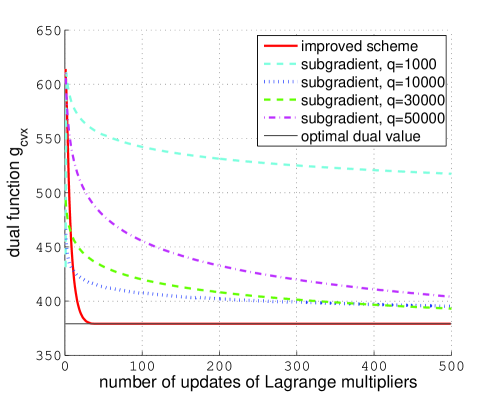
Figure 4: Comparison of convergence behaviour between subgradient dual decomposition approach, with different initial stepsizes $q$, and the improved dual decomposition approach, for CA-DSB

VI-B Convergence speed up for direct DSM

It was shown in [5] that for direct DSM algorithms the subgradient based dual decomposition approach with a particular stepsize selection procedure works well for ADSL scenarios, i.e. there are typically only 50-100 subgradient iterations needed to converge to the optimal dual variables. However for multi-user VDSL scenarios, which use a much larger frequency range and have to cope with significantly more crosstalk interference, existing subgradient approaches [4][5] are found to have significant convergence problems. We will focus on such VDSL scenarios and demonstrate how the improved approach succeeds in providing much faster convergence.

The different VDSL scenarios are shown in Figures 5, 6 and 8, i.e. four-user VDSL upstream, six-user VDSL upstream, and six-user VDSL upstream scenario with a subset of strong symmetric crosstalkers, respectively. The weights $w_{n}$ are chosen equal for all users $n$, namely $w_{n}=1/N$. Note that we used the multiple starting point procedure MS-DSB to solve the nonconvex per-tone problems for the subgradient based dual decomposition approach as well as the improved dual decomposition approach using (28). In [11] it was shown that this procedure provides globally optimal performance for practical ADSL and VDSL scenarios.

The first scenario, shown in Figure 5, is a four-user upstream VDSL scenario, consisting of two far-users with line length $1200$ m and two near-users with line length $300$ m. In the higher frequency range, there is a significant crosstalk coupling. This is a near-far scenario where spectrum management is crucial as to avoid significant performance degradation for the far-end users. Note that the near-end users form a subset of strong symmetric crosstalkers, in the high frequency range. As mentioned in Section V, this can cause significant convergence problems for the dual decomposition approach. In fact, simulations show that the subgradient methods in [5] and [4] fail to converge to the dual variables, i.e. after $20000$ iterations the complementarity conditions for some users are far from being satisfied. The main problem is that the stepsize selection procedure, which is a crucial component for fast convergence, is difficult to tune. For decreasing step sizes as proposed in [4], with different initial stepsizes, the procedure does not converge. For adaptive stepsizes, as proposed in [5], very small stepsizes are selected resulting in a very slow convergence ($>20000$ iterations). It is observed that for some users there is a fast convergence to the corresponding complementarity conditions whereas for other users convergence is very slow. The presence of the strong subset of symmetric crosstalkers, can lead to large changes in primal variables for small changes in dual variables, as discussed in Section V, if stepsizes are not tuned carefully. The improved approach of Algorithm 3, in contrary, converges very fast to the optimal dual and primal variables. In only $100$ iterations convergence is obtained, within an accuracy of $0.05\%$.

Figure 5: 4-user VDSL upstream scenario

The second VDSL upstream scenario, shown in Figure 6, consists of six users with different line lengths. Also for this large crosstalk scenario, the standard subgradient approaches [5][4] fail to converge to the optimal dual variables, i.e. after $10000$ iterations the complementarity conditions are far from being satisfied. Similarly to the scenario of Figure 5, one can observe very different convergence behaviour for the different users to the corresponding complementarity conditions, where typically for a few users convergence is very slow. The improved dual decomposition approach however converges to the optimal dual and primal variables in only $150$ iterations, within an accuracy of $0.05\%$. The optimal transmit powers are shown in Figure 7 for illustration.

Figure 6: 6-user VDSL upstream scenario

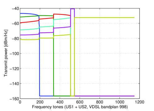
Figure 7: Optimal transmit powers for DSL scenario of Fig. 6 obtained using the improved dual decomposition approach. Blue, green, red, cyan, magenta and yellow curves correspond to transmit powers of users with line length $1200$m, $1000$m, $800$m, $600$m, $450$m and $300$m respectively.

The VDSL upstream scenario of Figure 8 consists of a six-line cable bundle with a subset of three strong symmetric crosstalkers, namely the set of lines with length $300$m. The standard subgradient approaches [5] [4] fail to converge to the optimal dual variables. The presence of the strong symmetric crosstalkers significantly slows down the convergence, as it can lead to multiple globally optimal solutions for particular values of the dual variables. Here, stepsize selection is very crucial as a small change in dual variables can lead to a large change in primal variables, as also explained in Section V. The improved dual decomposition approach converges to the optimal dual variables in only $150$ iterations, but does not succeed in obtaining the primal optimal variables, because of the existence of multiple globally optimal solutions (i.e. optimal transmit powers) for optimal dual variables that do not satisfy the user total power constraints. More specifically for this scenario, for the obtained optimal dual variables, the obtained transmit powers jump to different solutions, with total powers $\{P^{1},P^{2},P^{3}\}=\{P^{1,\mathrm{tot}},P^{2,\mathrm{tot}},P^{3,\mathrm{tot}}\}$, and $\{P^{4},P^{5},P^{6}\}\in\big{\{}\{3P^{\mathrm{tot}},A,A\},\{A,3P^{\mathrm{tot}},A\},\{A,A,3P^{\mathrm{tot}}\}\big{\}}$, with $A$ being very small. These primal solutions are shown in Figures 9, 10 and 11 . One can observe that in the low and medium frequency range (used tones 1-727), the users with line lengths $1200$ m, $900$ m and $600$ m are active. In this frequency range the strong crosstalkers will back-off and transmit at small similar transmit powers corresponding to a total power equal to $A$. However in the high frequency range (used tones 727-1147) where the users with line lengths $1200$ m, $900$ m and $600$ are switched off, the three strong crosstalkers will compete, where only one user can be active in each tone $k$ because of the significant crosstalk interference [30]. As explained in Section V, typical DSM algorithm implementations will select the same active user for each of these tones, namely the user that corresponds to the smallest dual variable, where the dual variable can be seen as a penalty. So instead of dividing the total power over the three users equally, which would lead to a primal solution satisfying the per-user total power constraints, one user gets all power, leading to $P^{n}=3P^{n,\mathrm{tot}}$ for user $n$ and $P^{m}=A$ for users $m\neq n$. Note that this prevents convergence to the optimal primal variables satisfying the per-user total power constraints.

However, when applying the proposed interleaving procedure (32), as proposed in Section V, together with the improved dual decomposition approach, we can observe a very fast convergence both in primal and dual variables. Convergence is achieved in only $150$ iterations, within an accuracy of $0.05\%$. The obtained optimal transmit powers are shown in Figure 12. In the frequency range between tone $728$ and tone $1147$, one can observe the interleaving effect. In Figure 13 this is zoomed in for tones $970$ up to $975$.

Remark: In the practical implementation the first step of the interleaving procedure is changed to ‘all best solutions that are 99.9% close to each other’. This is to prevent that the procedure is only active when the dual variables are exactly the same. The overall effect of this is a negligible noise on the transmit powers as can be seen in Figure 12.

Remark: Note that applying the interleaving procedure combined with the improved dual decomposition approach for the scenarios in Figures 5 and 6, also leads to a faster convergence in both dual and primal variables.

Figure 8: 6-user VDSL upstream scenario with subset of strong symmetric crosstalkers

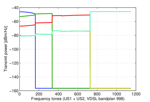
Figure 9: Transmit powers for DSL scenario of Fig. 8 for optimal dual variables $\mathbf{\lambda}^{*}$ and with user total powers $\{P^{1},P^{2},P^{3},P^{4},P^{5},P^{6}\}=\{P^{1,\mathrm{tot}},P^{2,\mathrm{tot}},P^{3,\mathrm{tot}},3P^{4,\mathrm{tot}},A,A\}$, where $A<<P^{4,\mathrm{tot}}$. Blue, green, red, cyan, magenta, yellow curves correspond to transmit powers of users 1,2,3,4,5 and 6 respectively.

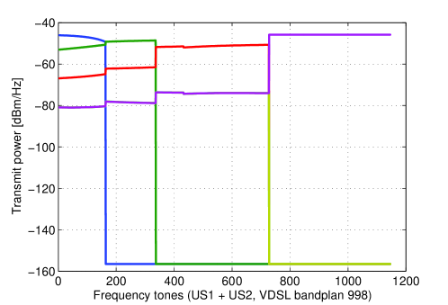
Figure 10: Transmit powers for DSL scenario of Fig. 8 for optimal dual variables $\mathbf{\lambda}^{*}$ and with user total powers $\{P^{1},P^{2},P^{3},P^{4},P^{5},P^{6}\}=\{P^{1,\mathrm{tot}},P^{2,\mathrm{tot}},P^{3,\mathrm{tot}},A,3P^{5,\mathrm{tot}},A\}$, where $A<<P^{5,\mathrm{tot}}$. Blue, green, red, cyan, magenta, yellow curves correspond to transmit powers of users 1,2,3,4,5 and 6 respectively.

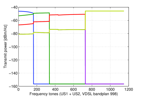
Figure 11: Transmit powers for DSL scenario of Fig. 8 for optimal dual variables $\mathbf{\lambda}^{*}$ and with user total powers $\{P^{1},P^{2},P^{3},P^{4},P^{5},P^{6}\}=\{P^{1,\mathrm{tot}},P^{2,\mathrm{tot}},P^{3,\mathrm{tot}},A,A,3P^{6,\mathrm{tot}}\}$, where $A<<P^{6,\mathrm{tot}}$. Blue, green, red, cyan, magenta, yellow curves correspond to transmit powers of users 1,2,3,4,5 and 6 respectively.

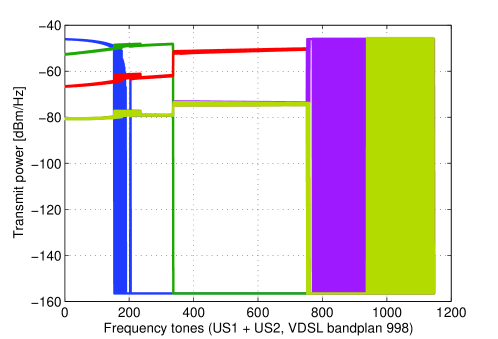
Figure 12: Transmit powers for scenario of DSL scenario of Fig. 8 obtained using improved dual decomposition approach with the interleaving procedure (32). Blue, green, red, cyan, magenta, yellow curves correspond to transmit powers of users 1,2,3,4,5 and 6 respectively.

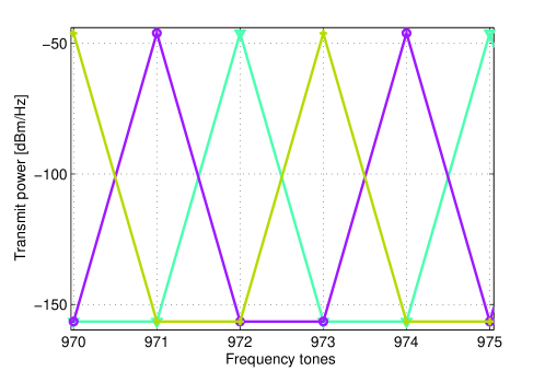
Figure 13: Zoom in on tones $970$ to $975$ of Fig. 12.

VII Conclusion

Dynamic spectrum management has been recognized as a key technology to significantly improve the performance of DSL broadband access networks by mitigating the impact of crosstalk interference. Existing DSM algorithms use a standard subgradient based dual decomposition approach to tackle the corresponding nonconvex optimization problems. However, this standard approach is often found to lead to extremely slow convergence or even no convergence at all. Especially for multiuser VDSL scenarios with subsets of strong symmetric crosstalkers significant convergence problems are observed because (1) the stepsize selection procedure of the subgradient updates is very critical, and (2) because special care must be taken when recovering the optimal transmit powers from the optimal dual solution. This paper proposes an improved dual decomposition approach, which consists of an optimal gradient based scheme with an automatic optimal stepsize selection removing the need for a tuning strategy. With this approach it is shown how the convergence of current state-of-the-art DSM algorithms, based on iterative convex approximations, is improved by one order of magnitude. The improved dual decomposition approach is also applied to other DSM algorithms (OSB, ISB, ASB, (MS)-DSB, MIW). The addition of an extra interleaving procedure for recovering the optimal transmit powers from the dual optimal solution furthermore improves the convergence of the proposed approach. Simulation results demonstrate that significant convergence speed ups are obtained using the proposed improved dual decomposition approach.

References

- [1] DSL Forum (www.dslforum.org), “DSL dominates global broadband subscriber growth,” Tech. Rep., March 2007, internet: http://www.broadband-forum.org/news/download/pressreleeases/YE06_Release.pdf.
- [2] K.B. Song, S.T. Chung, G. Ginis, J.M. Cioffi, “Dynamic spectrum management for next-generation DSL systems,” IEEE Communications Magazine, vol. 40, no. 10, pp. 101–109, Oct. 2002.
- [3] R. Cendrillon, W. Yu, M. Moonen, J. Verlinden and T. Bostoen, “Optimal multiuser spectrum balancing for digital subscriber lines,” IEEE Trans. Comm., vol. 54, no. 5, pp. 922–933, May 2006.
- [4] W. Yu and R. Lui, “Dual methods for nonconvex spectrum optimization of multicarrier systems,” IEEE Trans. on Comm., vol. 54, no. 7, July 2006.
- [5] P. Tsiaflakis, J. Vangorp, M. Moonen, J. Verlinden, “A low complexity optimal spectrum balancing algorithm for digital subscriber lines,” Signal Processing, vol. 87, no. 7, pp. 1735–1753, July 2007.
- [6] P. Tsiaflakis, Y. Yi, M. Chiang, M. Moonen, “Green DSL: Energy-Efficient DSM,” in accepted for publication in IEEE International Conference on Communications (ICC 2009), June 2009.
- [7] M. Wolkerstorfer, D. Statovci, and T. Nordström, “Dynamic spectrum management for energy-efficient transmission in dsl,” in The Eleventh IEEE International Conference on Communications Systems (ICCS 2008), Guangzhou, China, November 2008.
- [8] J. M. Cioffi, S. Jagannathan, W. Lee, H. Zou, A. Chowdhery, W. Rhee, G. Ginis, P. Silverman, “Greener copper with dynamic spectrum management,” in AccessNets, Las Vegas, NV, USA, Oct 2008.
- [9] Z. Q. Luo, S. Zhang, “Dynamic Spectrum Management: Complexity and Duality,” IEEE Journal of Selected Topics in Signal Processing, vol. 2, no. 1, pp. 57–73, Feb. 2008.
- [10] P. Tsiaflakis, Y. Yi, M. Chiang, M. Moonen, “Throughput and delay of DSL dynamic spectrum management with dynamic arrivals,” in IEEE Global Telecommunications Conference (GLOBECOM), November 2008, pp. 1–5.
- [11] P. Tsiaflakis, M. Diehl, M. Moonen, “Distributed Spectrum Management Algorithms for Multiuser DSL Networks,” IEEE Transactions on Signal Processing, vol. 56, no. 10, pp. 4825–4843, Oct 2008.
- [12] Y. Xu, T. Le-Ngoc, S. Panigrahi, “Global concave minimization for optimal spectrum balancing in multi-user dsl networks,” IEEE Transactions on Signal Processing, vol. 56, no. 7, pp. pp. 2875–2885, July 2008.
- [13] R. Cendrillon, M. Moonen, “Iterative spectrum balancing for digital subscriber lines,” in IEEE Int. Conf. on Communications, vol. 3, no. 3, May 2005, pp. 1937–1941.
- [14] J. Papandriopoulos and J. S. Evans, “Low-complexity distributed algorithms for spectrum balancing in multi-user DSL networks,” in IEEE Int. Conf. on Communications, vol. 7, June 2006, pp. 3270–3275.
- [15] W. Yu, “Multiuser water-filling in the presence of crosstalk,” in Information Theory and Applications (ITA), Feb. 2007.
- [16] R. Cendrillon, J. Huang, M. Chiang, M. Moonen, “Autonomous spectrum balancing for digital subscriber lines,” IEEE Trans. on Signal Processing, vol. 55, no. 8, pp. 4241–4257, August 2007.
- [17] S. Jagannathan and J. M. Cioffi, “Distributed Adaptive Bit-loading for Spectrum Optimization in Multi-user Multicarrier Systems,” Elsevier Physical Communication, vol. 1, no. 1, pp. pp. 40–59, 2008.
- [18] W. Yu, G. Ginis, J. Cioffi, “Distributed multiuser power control for digital subscriber lines,” IEEE J. Sel. Area. Comm., vol. 20, no. 5, pp. 1105–1115, Jun. 2002.
- [19] I. Necoara, J.A.K. Suykens, “Application of a smoothing technique to decomposition in convex optimization,” IEEE Transactions on Automatic Control, vol. 11, no. 53, pp. 2674–2679, 2008.
- [20] Y. Nesterov, Introductory Lectures on Convex Optimization: A Basic Course, Kluwer, Ed. Boston, 2004.
- [21] T. Starr, J. M. Cioffi, P. J. Silverman, Understanding digital subscriber lines. Prentice Hall, 1999.
- [22] R. Lui and W. Yu, “Low-complexity near-optimal spectrum balancing for digital subscriber lines,” in IEEE Int. Conf. on Communications, vol. 3, no. 3, May 2005, pp. 1947–1951.
- [23] W. Lee, Y. Kim, M. H. Brady and J. M. Cioffi, “Band-preference dynamic spectrum management in a DSL environment,” in IEEE Glob. Telecomm. Conf., Nov. 2006, pp. 1–5.
- [24] M. Chiang, C.W. Tan, D.P. Palomar, D. O’Neill, D. Julian, “Power control by geometric programming,” IEEE Transactions on Wireless Communications, vol. 6, no. 7, pp. 2640–2651, July 2007.
- [25] S. Kontogiorgis, R. D. Leone, and R. Meyer, “Alternating direction splitings for block angular parallel optimization,” Journal of Optimization Theory and Applications, vol. 90, no. 1, pp. 1–29, 1996.
- [26] G. Chen and M. Teboulle, “A proximal-based decomposition method for convex minimization problems,” Mathematical Programming (A), vol. 64, pp. 81–101, 1994.
- [27] J. E. Spingarn, “Applications of the method of partial inverses to convex programming: decomposition,” Mathematical Programming (A), vol. 32, pp. 199–223, 1985.
- [28] P. Tsiaflakis, C.W. Tan, Y. Yi, M. Chiang, M. Moonen, “Optimality certificate of dynamic spectrum management in multi-carrier interference channels,” in IEEE International Symposium on Information Theory, July 2008, pp. 1298–1302.
- [29] L. Xiao, M. Johansson, S. Boyd, “Simultaneous Routing and Resource Allocation via Dual Decomposition,” IEEE Transactions on Communications, vol. 52, no. 7, pp. 1136–1144, July 2004.
- [30] S. Hayashi, Z. Q. Luo, “Dynamic spectrum management: When is FDMA sum-rate optimal?” in IEEE Int. Conf. on Acoustics, Speech and Sign. Proc., vol. 3, April 2007, pp. III–609 – III–612.