Is Europe Evolving Toward an Integrated Research Area?

An integrated European Research Area (ERA) is a critical component for a more competitive and open European R&D system. However, the impact of EU-specific integration policies aimed at overcoming innovation barriers associated with national borders is not well understood. Here we analyze $2.4\times 10^{6}$ patent applications filed with the European Patent Office (EPO) over the 25-year period 1986–2010 along with a sample of $2.6\times 10^{5}$ records from the ISI Web of Science to quantitatively measure the role of borders in international R&D collaboration and mobility. From these data we construct five different networks for each year analyzed: (i) the patent co-inventor network, (ii) the publication co-author network, (iii) the co-applicant patent network, (iv) the patent citation network, and (v) the patent mobility network. We use methods from network science and econometrics to perform a comparative analysis across time and between EU and non-EU countries to determine the “treatment effect” resulting from EU integration policies. Using non-EU countries as a control set, we provide quantitative evidence that, despite decades of efforts to build a European Research Area, there has been little integration above global trends in patenting and publication. This analysis provides concrete evidence that Europe remains a collection of national innovation systems.

Efforts towards European research and development (R&D) integration have a long history, intensifying with the Fifth Framework Program (FP) in 1998  (?, ?, ?) and the launch of the European Research Area (ERA) initiative at the Lisbon European Council in 2000. A key component of the European Union (EU) strategy for innovation and growth  (?, ?) is the ERA aims at an integrated innovation system through directed funding, increased mobility, and streamlined innovation policies that can overcome national borders.

To assess the rate of progress towards this ERA vision, we analyze the evolution of geographical collaboration networks constructed from patent and scientific publication data. While these data may not capture every facet of ERA, they are widely accepted measures of R&D output and the European Commission considers them crucial for the evaluation of the Horizon 2020 FP  (?). All in all, we find no evidence since 2003 that EU innovation policies aimed at promoting an integrated research and innovation system have corresponded to intensified cross-border R&D activity in Europe vis-à-vis other OECD countries.

We exploit the June 2012 release of the OECD REGPAT database  (?), and analyze all $\sim 2.4\times 10^{6}$ patent applications filed with the European Patent Office (EPO) over the period 1986-2010. For comparison with scientific publications we take a random sample of $\sim 2.6\times 10^{5}$ records from the ISI Web of Science over the period 1991-2009. We geo-coded each data set at the NUTS3 region level (see Supplementary Materials (SM)). Using the data we construct 5 networks, which provide different perspectives into EU R&D integration. In our networks, nodes correspond to NUTS3 regions and links represent collaboration/mobility measures. Specifically, (i) the patent co-inventor network and (ii) the publication co-author network measure the intensity of inter-regional collaboration at the individual level; (iii) the co-applicant patent network measures the collaboration between institutions (“applicants”) located in different regions; (iv) the patent citation network indirectly measures scientific integration by following the flow of citations from patents in one region to patents in another; (v) the patent mobility network measures the mobility of inventors from one region to another by tracking their location in subsequent patents.

We use a standard network-clustering algorithm to identify communities, i.e., sub- sets of nodes more strongly linked to one another than to nodes outside, to compare geopolitical borders and R&D networks. Regional integration is shown in Fig. 1 in the purple community, centered on Eindhoven, which is composed of strongly collaborating regions in the Benelux, and in the international Nordic community with its center in Copenhagen. Despite these exceptions, patterns of co-inventorship in Europe continue to be largely shaped by national borders. This observation stands in contrast to the community structure of the highly dispersed “coast-to-coast” US co-inventor network (see SM for comparison)  (?). Figure 1 shows Europe as a collection of regional and national innovation communities. However, that does not necessarily mean that integration efforts have been unsuccessful. The more relevant question, then, is at what rate is Europe evolving toward an integrated research system relative to the rate of cross-border R&D collaboration observed in non-EU OECD countries.

Consistent with recent studies  (?, ?, ?, ?) we observe a significant increase in the total number of cross-border research collaborations, both within and outside Europe (see SM). To assess the role of EU-specific factors, we compare the relative change in cross-border collaboration between European countries (e.g., distinguishing German-French, from German-German, and French-French collaborations) to the relative change in cross-border collaboration between non-European OECD countries (e.g., distinguishing USA-Japan from USA-USA, and Japan-Japan collaborations). Collaborations between EU and non-EU regions are not included in our analysis.

For each network, our econometric model simultaneously performs three quantitative differences and controls for the size of regions, geographic distance and time effects (see SM). First, the difference between cross-border and intra-border average number of links is computed, both for EU and non-EU OECD nations. Second, the difference between these two estimates isolates the impact of EU-specific factors on R&D integration. The final one, to a baseline year, yields the quantitative output of the model, i.e. the expected number of additional links between regions resulting from EU specific factors. This quantity is shown in Figure 2. Comparing data points from two different years, a higher y-axis value indicates a greater impact of EU specific factors upon integration among EU nations. Thus by construction, choice of the baseline year does not alter our results. It also follows that a positive (negative) slope indicates Europe is integrating faster (slower) than non-EU countries.

Since the late 1990s, we observe some signs of integration in European patent statistics. In the case of the patent co-inventor network, there has been an increase in cross-border collaboration in Europe vis-à-vis other OECD countries. This effect was relatively pronounced from 1998 to 2002, but stalled in 2003. Since then, the additional number of links for an average pair of regions due to Europe specific factors has never been significantly larger than zero. The patent co-applicant network exhibits no significant increase since 1996. The citation network shows a temporary bump in integration in the late 90’s, then fluctuates around that level. Finally, the inventors’ mobility network shows almost no progress in the last decade, confirming a slow pace of integration for the European high-skill labor market.

The scientific publications co-authorship network shows a negative trend since 1999, indicating that cross-border links among non-EU OECD countries grew faster than European cross-border links. These results are striking and deserve further investigation given the amount of resources the EU has committed to promote cross-border scientific collaboration through programs like FPs, European Cooperation in Science and Technology, Networks of Excellence, Marie Curie Actions, etc.

In sum, our analysis of R&D patent and publication networks shows Europe remains a collection of loosely coupled national innovation systems  (?). Furthermore, since 2003, cross-border collaborations in Europe have developed no faster than in the rest of the OECD countries. Several ongoing initiatives seek to address a number of general shortcomings that have affected previous integration efforts  (?). The European Institute of Innovation and Technology’s (EIT) Knowledge and Innovation Communities are long-term (7-15 years) collaboration networks spanning all aspects of the R&D ecosystem  (?). To foster synergetic interaction between national funding bodies, Science Europe, an association of national research organizations, was founded in 2011  (?).

The European Research Council  (?) has taken major steps to promote cross-border mobility by making grants competitive and portable. Likewise, a memorandum of understanding signed by the European Commission and the League of European Research Universities  (?) pushes for pension unification and transparency in hiring and tenure decisions.

Despite these initiatives to increase competition within the system, monitoring and evaluation must drastically change if Europe is to accomplish its ambitious goals in Science and Technology. Evidence based evaluation focused on output and impact is crucial, as recognized in the plans for the Horizon 2020 FP  (?). Our methodology promotes this vision by combining interdisciplinary expertise with data relevant to evaluation.

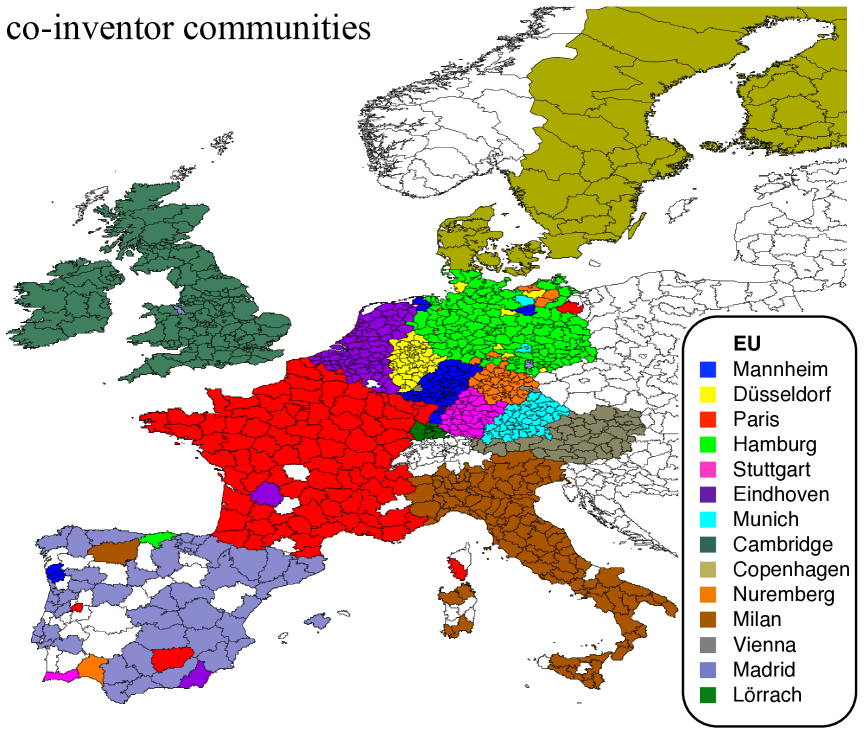
Figure 1: The community structure of the 2009 EU-15 co-inventor network. Communities are shown with different colors and are labeled by their most central region. Communities have been generated by iteratively aggregating nodes (NUTS3 regions) into clusters of increasing size (see SM). Blank regions have no ties in 2009.

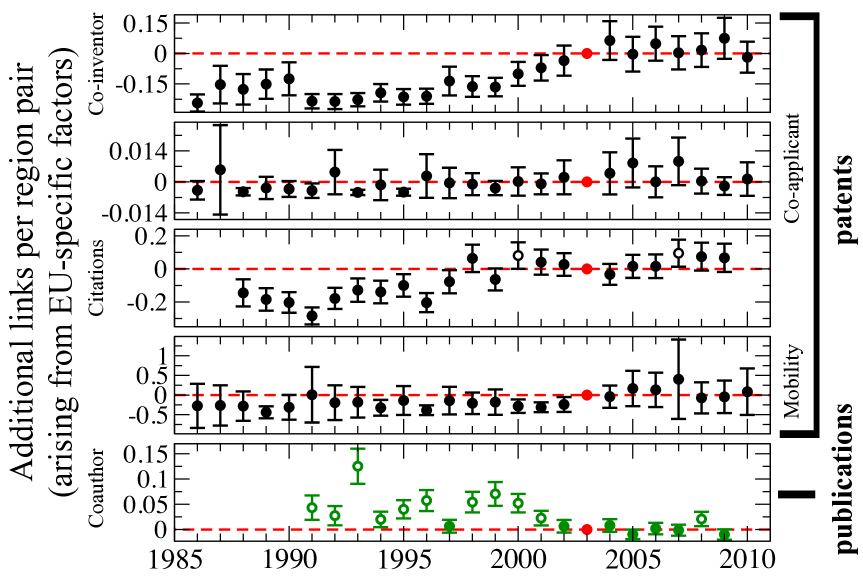
Figure 2: The evolution of European integration in five R&D networks. We use econometric methods to measure the effect of EU specific factors on the amount of cross-border links relative to within-border links and to the rest of non-EU OECD countries. Results are shown for 4 different patent networks (black circles) and a scientific publication network (green circles). Open circles indicate statistically significant (.05 level) positive deviations from the baseline year (2003). The y-axis reports the additional number of links for an average pair or regions relative to 2003 due to R&D integration in Europe.

Supplementary Materials

Is Europe Evolving Toward an Integrated Research Area?

Alessandro Chessa,¹ Andrea Morescalchi,¹ Fabio Pammolli,¹

Orion Penner,¹ Alexander M. Petersen,¹ Massimo Riccaboni,¹

¹IMT Institute for Advanced Studies Lucca, 55100 Lucca, Italy

(Feb. 11, 2013)

1 Materials and Methods

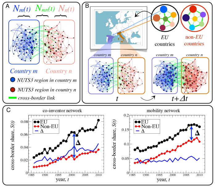
Figure S1: Network analysis of co-patent activity. (A) Schematic illustration of the network methodology. For each year $t$ we calculate weighted links from $N_{n}(t)$, the number of patents between NUTS3 regions within a country $n$, and $N_{mn}(t)$, the number of patents between NUTS3 regions in different countries, as indicated by the green links. (B) The evolution of the collaboration networks over time serves as the basis for analyzing the integration rate of the EU innovation system, and these within-EU changes over time are compared to non-EU changes over time. (C) For the set of EU countries, we show the annual cross-border share $S(t)=N_{\times}/N_{T}$, calculated as the ratio of the number $N_{\times}(t)=\sum_{m,n}N_{mn}$ of cross-border collaboration links divided by the total number $N_{T}(t)=N_{\times}+\sum_{n}N_{n}$ of both intra- and cross-border collaboration links. We calculate the same quantity for the set of non-EU countries. The increase of S over time in the co-inventor and mobility networks reflects a well-documented increasing trend in global patent activity. However, the share difference $\Delta=S(EU)-S(nonEU)$, a coarse indicator of relative integration that does not control for EU specific factors, is relatively flat for both measures, except for a small “jump” around 1998-2000 in the co-inventor network. The relatively constant trend in $\Delta(t)$ is preliminary empirical evidence that brings into question the effectiveness of EU policies aimed at accelerating integration. Our econometric “treatment effect” approach further investigates the effectiveness of EU integration policies by controlling for multiple underlying variables, see Eq. S5. Link count values are listed in Table S1.

We perform a geo-spatial network analysis of scientific collaboration. In our framework, the nodes are NUTS3 regions. In our analysis of R&D integration, we distinguish between two types of collaboration links: (a) links between NUTS3 within the same country, and (b) cross-border links between NUTS3 regions in country $m$ and NUTS3 regions in country $n$, as demonstrated by the green links in Fig. S1(A). Fig. S1(B) outlines our methodological approach where we analyze and compare the time evolution of collaboration networks in EU countries vis-à-vis non-EU countries. We use an econometric model to measure the difference between the network structure in year $t^{*}+\Delta t$ and the “baseline year”, which we choose to be $t^{*}=2003$.

Supplementary materials are organized as follows: the first section describes our data sources and database construction; the second section illustrates the network clustering methods we employed; and the third section contains a detailed description of our statistical methodology and results. All relevant Data and Code can be downloaded at:
http://cse.lab.imtlucca.it/SOM/SOM.zip

1.1 Data

Patent collaboration data are drawn from the OECD REGPAT database  (?, ?) which compiles all patent applications filed with the European Patent Office (EPO) since the 1960s. Within this database the geographical location of inventor and applicant are designated by one of the 5,552 NUTS3 regions in 50 countries. We use all patent applications across all classes in the REGPAT database over the period 1986–2010, $~{}2.4\times 10^{6}$ applications overall. We construct 4 geographical networks: (i) co-inventors, (ii) co-applicants, (iii) citations and (iv) inventor mobility. In (i) and (ii) the strength of a link between two regions is equal to the number of patents jointly invented by or jointly assigned to the two regions. In (iii) it is the number of patent citations between inventors’ regions. Specifically, for each pair $(i,j)$ of NUTS3 regions we count the number of times that (a patent invented by an inventor residing in) region $i$ cites (a patent invented by an inventor residing in) region $j$. Conversely the number of citations that $i$ receives from $j$ is the strength of the link $(j,i)$. In (iv) link weight is equal to the number of inventors moving from region $i$ to region $j$. As for citations, the mobility network is directed, i.e. we distinguish between mobility from $i$ to $j$ and mobility in the opposite direction, $j$ to $i$. Links are created tracking regional migration for inventors with at least two patents. We compare the affiliation of inventors’ consecutive patents and assign a new link whenever a new patent is filed in a region different from the one reported in the inventor’s previous patent.

Fig. S1(C) illustrates the global trend of increased cross-border collaboration in the co-inventor network, and increased cross-border flow in the mobility network. We count the total number of intra-border collaborations links $N_{i}=\sum_{n}N_{n}(t)$ and the total number of cross-border collaboration links $N_{\times}=\sum_{m,n}N_{m,n}$ and define the collaboration share to be the ratio $S\equiv N_{\times}/(N_{i}+N_{\times}$) for a given time period (values shown in Fig. S1(C) and values for the other networks are listed in Table S1). The overall increasing trend reflects both the increasing pace of patenting and the decreasing role of distance in worldwide research efforts. We note that for the case of Europe the 15% final share matches the ratio of the EU research budget to the combined national research budgets of EU nations.

Scientific publications data are drawn from ISI-Web of Science. The Web of Science database is a bibliographical collection maintained by Thomson Reuters, considered to be one of the most comprehensive and reliable sources of information on research activity across all fields of science. We analyze a random sample of 256,015 research articles in the period 1991-2009 by authors affiliated at institutions located in the OECD countries. We build the regional co-authorship network by geo-coding each address attached to the paper. Since addresses refer to institutional affiliations and it is not possible to link individuals to organizations  (?), we define co-authorship as the co-occurrence of two or more addresses on a publication. Therefore, if an author lists multiple affiliations in different regions we consider co-authorship links between those regions in our analysis.

1.2 Community detection

There are now many community detection methods for clustering networks  (?), one the most popular being modularity optimization, introduced by Newman and Girvan  (?). Some limitations have been noted for this method, the most important being the existence of a resolution limit  (?) that prevents it from detecting small modules. Nevertheless it is reliable for standard cluster analysis provided a suitable optimization procedure is employed. In the present analysis we adopt a weighted version of the modularity function and optimized it using the Louvain algorithm  (?). This algorithm arrives at the final community structure by starting from isolated nodes (NUTS-3 regions in our case) and iteratively aggregating them into communities of increasing size. This particular optimization procedure can mitigate the effect of the resolution limit.

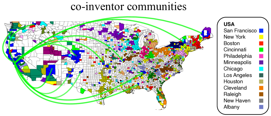
Figure S2: Community structure of the 2009 USA co-inventor network. We show only the top 13 communities and left regions belonging to all other communities white. The most central region of each community is listed in the legend and is determined by the procedure described in Section 2. Communities were determined using the Newman Girvan algorithm (21) and the Louvain algorithm (23). The green arcs are used to highlight some of the long distance members of the community for which San Francisco is the core region. Source: our computations based on data and code available here: http://cse.lab.imtlucca.it/SOM/SOM.zip

After determining the community structure we calculated the centrality of each node within a community using a novel perturbative approach. Since we obtain the modularity score of a network ($Q$) by an optimization procedure, every perturbation of the partition structure leads to a negative variation in the modularity ($dQ$). For every node we calculate a $dQ$ by moving the node into every other community in the network. Within a specific community, the node with the most negative $dQ$ is defined as the most central node (core region). The legends of Fig. 1 in the manuscript and Fig. S2 below identify the most central nodes (using the city name associated with the NUTS3 region) for the top 13 communities in the 2009 co-inventor networks, for Europe and the USA respectively.

The community structure of the top 13 communities in the USA co-inventor network in 2009 is shown in Fig. S2. Green arcs have been added to highlight (some of) the long range connections of the community for which San Francisco is the most central region. Communities in the USA have a higher fraction of cross border links than in the EU, indicating drastically different levels of integration in their respective R&D collaboration networks. This result is confirmed numerically by comparing the share of links with at least one region outside of the nation in which the core region is located for Europe versus the share of links with at least on member outside the state in which the core region is located for US communities. This share is always significantly higher in the US co-inventor than in the EU. Table S2 shows that the fraction of cross-border ties is on average larger for the US ($0.706$) as compared to the EU ($0.138$), with $t$-statistic 7.16 ($p<0.01$). The only European cluster which has a cross-border connectivity comparable with the US ones is the Nordic cluster centered on Copenhagen, which has many members outside Denmark in Sweden and Finland.

1.3 Statistical analysis

The rate at which EU (NUTS3) regions are linking to regions in other EU countries is increasing due to two types of factors: those that are global and those that are EU specific. Thus, to capture the effect of EU specific institutional factors we must account for the net effect of the global factors. In technical terms, we use the non-EU OECD members as a control group and its behaviour serves as the counterfactual behavior of EU regions.

In our statistical analysis the number of links ($y_{i}\equiv A_{k,l}$) between NUTS3 regions $k$ and $l$ is regressed on a set of independent variables. We model this dependent variable with a count density. A number of models can be found in the literature to handle count densities, including the Poisson model, Negative Binomial model variants, and Zero-inflated models  (?, ?, ?, ?, ?, ?, ?). Since $\sim 90\%$ of our link counts are zero, we opted for a zero-inflated negative binomial (ZINB), as consistent with  (?, ?). Zero-inflated models allow zeros to be generated by two distinct processes and are generally used when data exhibits “excess zeros”  (?). The ZINB model supplements a count density, $\tilde{P}$ with a binary zero generating process $\psi$. This allows a zero count to be produced in two ways, either as an outcome of the zero generating process with probability $\psi$, or as an outcome of the count process $\tilde{P}$ provided the zero generating process did not produce a zero ($\psi_{i}=1$).

The density distribution for the count pair $y_{i}$ is then given by

$$P(y_{i})=(1-\psi_{i})*\tilde{P}(y_{i}),$$ (S1 )

where the zero generating process $\psi_{i}$ is parameterized as a logistic function of the regressors in $Z_{i}$, with parameter vector $\beta^{0}$:

$$\psi_{i}=\frac{\exp(Z_{i}\beta^{0})}{1+\exp(Z_{i}\beta^{0})}.$$ (S2 )

The count process $\tilde{P}(y_{i})$ is modeled as Negative Binomial of the second kind (NB2):

$$\tilde{P}(y_{i})=\frac{\Gamma(y_{i}+\alpha^{-1})}{\Gamma(y_{i}+1)+\Gamma(\alpha^{-1})}\left(\frac{\alpha^{-1}}{\alpha^{-1}+\mu_{i}}\right)^{\alpha^{-1}}\left(\frac{\mu_{i}}{\alpha^{-1}+\mu_{i}}\right)^{y_{i}},$$ (S3 )

where the conditional mean $\mu_{i}$ is parameterized as an exponential function of the linear index $X\beta^{1}$, and $\alpha(\geq 0)$ is the overdispersion parameter. Thus, drawing together equations S1, S2, and S3 our model for the expected count is

$$E(y_{i}|X_{i},Z_{i})=\left(1-\frac{\exp(Z_{i}\beta^{0})}{1+\exp(Z_{i}\beta^{0})}\right)*\exp(X_{i}\beta^{1}).$$ (S4 )

In our estimation procedure we assume $X_{i}=Z_{i}$ because there is no reason to expect some variables would be relevant only in one of the two processes. However, individual regressors can impact the $y_{i}$ estimator differently through the two distinct processes and their separate parameter vectors, $\beta^{0}$ and $\beta^{1}$.

The linear indices $X\beta^{0}$ for the zero-generating process and $X\beta^{1}$ for the Negative Binomial process are modeled in parallel as

$$\begin{split}X\beta^{j}&=\beta_{0}^{j}+\beta_{1}^{j}border+\beta_{2}^{j}eu+\beta_{3}^{j}Distance+\beta_{4}^{j}Size_{k}+\beta_{5}^{j}Size_{l}+\gamma^{j}border*eu+\\ &+\sum_{t=2}^{T}\theta_{t}^{j}year_{t}+\sum_{t=2}^{T}\delta_{t}^{j}border*year_{t}+\sum_{t=2}^{T}\zeta_{t}^{j}eu*year_{t}+\sum_{t=2}^{T}\eta_{t}^{j}border*eu*year_{t},\end{split}$$ (S5 )

where $j=0,1$. $Size_{k}$ and $Size_{l}$ denote the size of each of the two regions. We proxy the size of a region by the total number of links attached to the region. $Distance$ is the geographical distance between centroids of the regions and $year_{t}$ is the year dummy variable. The time interval for estimation is generally 1986-2010 for patents and 1991-2009 for publications. $border$ flags pairs of NUTS3 regions within the same country. $eu$ flags pairs of NUTS3 regions that are within the EU ($eu=1$) and pairs of NUTS3 regions for which neither are in the EU ($eu=0$). Cross-sections are pooled over years and estimation is carried out on the whole sample clustering standard errors at pairs of NUTS3 regions. Following the Difference-in-Differences (DiD) econometric strategy, the full set of double/triple interaction dummy variables among the three dimensions ($eu=\{0,1\}$, $border=\{0,1\}$, $year_{t}=\{0,1\}$ for $t=2,\ldots,T$) is relevant to the identification of treatment effect.

In the literature on program evaluation, DiD estimation is one of the most popular strategies for identifying the impact of a policy or treatment  (?, ?, ?, ?). Treatment effect on an outcome variable is, in general, defined as the difference between the outcome actually observed under the treatment and the counterfactual, that is the outcome that would have been observed without treatment  (?). Under this treatment-effect framework, our analysis seeks to quantify the effect of EU institutional changes upon integration within the EU, by measuring the relative rate of cross-border links within a given network. Moreover, to isolate the signal arising only from EU factors we must control for the global rate of cross-border integration. Specifically, we extend the standard DiD strategy of one state indicator (treatment vs control group) to the case of two state indicators, providing a control group of links between non-European countries. For the purpose of embedding the institutional comparison in a temporal perspective, our analysis also includes a time variable, in line with the standard treatment-effect formalism. Due to the addition of a second state indicator our approach is a Difference-in-Differences-in-Differences estimator (DiDiD)  (?).

While the standard version of DiD estimation is designed for the linear case, it can be extended to cases in which the outcome variable is non-continuous and nonlinear estimation is preferred, as in our case  (?). When employing the ZINB model it is not possible to make a general statement regarding the sign of the treatment effect merely by checking the sign of the interaction term(s) coefficients. However, we can identify the treatment effect by calculating the incremental effect of the interaction term through comparison of a given year to a baseline year. In our framework, treatment effects are incremental effects of the triple interaction terms $border*eu*year_{t}$, evaluated at means of the regressors.

Denoting the actual and counterfactual outcomes of our count dependent variable as $Y^{1}$ and $Y^{0}$ respectively and taking into account our DiDiD extension, the yearly treatment effect ($\tau_{t}$) can be defined as

$$\begin{split}\tau_{t}(year_{t}=1,eu=1,border=1,M)=&E[Y^{1}|year_{t}=1,eu=1,border=1,M]\\ &-E[Y^{0}|year_{t}=1,eu=1,border=1,M],\end{split}$$ (S6 )

where $M$ is the matrix of controls ($Size_{k},Size_{l},Distance$). Given the linear indices modeled in Eq. S5 the expectation values of $Y^{1}$ and $Y^{0}$, for the group under treatment are

$$\begin{split}E[Y^{1}|year_{t}=1,&eu=1,border=1,M]=\\ &\frac{\exp(\phi^{1}+\omega^{1}M+\eta_{t}^{1})}{1+\exp(\phi^{0}+\omega^{0}M+\eta_{t}^{0})},\end{split}$$ (S7 )

$$\begin{split}E[Y^{1}|year_{t}=1,&eu=1,border=1,M]=\\ &\frac{\exp(\phi^{1}+\omega^{1}M)}{1+\exp(\phi^{0}+\omega^{0}M)},\end{split}$$ (S8 )

where $\phi^{j}\equiv\beta_{0}^{j}+\beta_{1}^{j}+\beta_{2}^{j}+\gamma^{j}+\theta_{t}^{j}+\delta_{t}^{j}+\zeta_{t}^{j}$, and where $\omega^{1}$ and $\omega^{0}$ are the coefficient vectors for $M$ (the controls). We can then write Eq. S6 as

$$\tau_{t}(year_{t}=1,eu=1,border=1,M)=\frac{\exp(\phi^{1}+\omega^{1}M+\eta_{t}^{1})}{1+\exp(\phi^{0}+\omega^{0}M+\eta_{t}^{0})}-\frac{\exp(\phi^{1}+\omega^{1}M)}{1+\exp(\phi^{0}+\omega^{0}M)}.$$ (S9 )

We calculate the yearly treatment effect $\tau_{t}$ in Eq. S9 using parameter estimates of $\beta^{0}$ and $\beta^{1}$ and the sample mean of $M$. Estimates for the parameters in vectors $\beta^{0}$ and $\beta^{1}$ are obtained through maximum likelihood. Although differences in the linear indices ($\eta_{t}^{1}$ and $\eta_{t}^{0}$) are constant across individuals for a given t, it is clear from Eq. S9 that differences in the dependent variable depend on the values chosen for $M$.

Relative to the baseline year $t^{*}$ (we use the year 2003 in our analysis as indicated by red dots in Fig. 2 in the manuscript), the yearly treatment effect reflects the impact of changes in institutional factors specific to the EU which have taken place in a given year $t$. Estimates of $\tau$, which are just marginal effects of the triple interaction term $border*eu*year_{t}$. Estimates are obtained averaging over all the variables in the model and thus refer to an “average” pair of regions.

Due to the large number of zero entries, in the regression analysis we ignore regions with fewer than 50 total patents. For inventor mobility, the analysis focuses only on NUTS3 region pairs with at least one link (nonzero counts). Since in co-authorship network the fraction of zeros is lower, we do not use any cutoff.

Table S1: Network data summary. Total numbers of intra-border and cross-border links calculated for each area by networks. Source: our computations based on data and code available here: http://cse.lab.imtlucca.it/SOM/SOM.zip

	REGPAT				REGPAT				REGPAT				REGPAT				ISI Publications
	Coinventor				Coapplicant				Citations				Mobility				Coauthor
	EU links		non-EU links		EU links		non-EU links		EU links		non-EU links		EU links		non-EU links		EU links		non-EU links
	Intra	Cross	Intra	Cross	Intra	Cross	Intra	Cross	Intra	Cross	Intra	Cross	Intra	Cross	Intra	Cross	Intra	Cross	Intra	Cross
1986	34,827	859	55,153	511	1,415	915	1,216	42	31,567	11,643	52,205	16,437	1,605	140	2,099	75
1987	38,526	1,077	62,617	595	1,569	884	1,390	38	35,150	15,371	60,750	21,111	1,807	171	2,503	95
1988	43,512	1,325	75,417	790	1,701	1,301	1,746	84	42,843	19,359	81,566	27,388	2,083	170	3,255	143
1989	50,462	1,596	91,458	1,005	1,869	1,456	1,870	94	51,360	23,520	101,107	33,281	2,666	222	3,824	147
1990	54,636	2,095	105,193	1,216	1,966	1,305	2,278	93	55,072	26,822	121,120	40,673	2,909	253	5,586	198
1991	47,755	1,521	104,199	1,246	1,618	1,141	2,139	91	55,263	26,743	134,172	45,161	2,824	272	5,860	250	2,112	582	10,230	774
1992	54,524	2,164	112,028	1,687	1,594	1,322	2,252	152	55,367	27,424	150,384	49,265	3,204	309	6,061	321	3,519	1,674	11,376	1,115
1993	53,864	1,933	109,058	1,818	1,373	907	2,070	187	57,098	28,976	149,610	47,845	3,096	314	5,930	311	3,792	2,296	13,376	1,495
1994	57,712	2,328	117,467	2,070	1,644	981	2,260	164	54,747	27,143	146,215	53,723	3,352	341	6,700	388	4,850	1,856	16,324	2,205
1995	68,499	3,014	135,726	3,218	1,994	1,050	2,719	246	51,941	28,434	151,797	51,539	3,903	451	7,791	511	3,820	1,808	17,727	2,054
1996	71,140	3,465	143,689	3,147	1,850	934	2,772	225	59,429	27,847	171,307	56,276	4,015	480	8,575	614	5,074	2,674	20,550	2,668
1997	84,402	4,464	165,497	4,271	2,247	881	2,965	251	51,943	28,495	163,503	53,387	4,805	604	9,409	677	7,571	2,962	25,651	3,336
1998	95,005	4,933	189,313	4,135	2,422	745	3,516	366	42,487	27,389	176,398	59,144	5,217	674	10,342	842	8,929	3,561	42,094	4,913
1999	105,492	6,611	206,325	5,226	2,892	748	3,658	362	42,202	27,138	166,953	57,620	5,739	802	11,418	898	13,434	5,187	41,402	4,595
2000	116,113	7,869	236,805	6,585	2,896	775	4,587	383	42,440	28,039	181,899	60,933	6,485	859	13,086	1,128	17,210	6,627	48,664	6,085
2001	131,038	8,827	289,700	6,253	2,795	877	5,600	476	41,729	25,933	184,064	65,369	6,935	1,035	15,080	1,283	18,558	8,514	45,597	7,226
2002	137,527	8,522	305,854	7,862	3,071	1,027	4,988	377	39,678	25,410	189,116	67,793	7,122	1,114	14,675	1,495	18,146	7,740	46,694	6,944
2003	140,980	9,900	295,097	8,549	2,768	1,131	5,242	478	41,395	26,393	167,170	69,722	7,078	1,223	15,783	1,621	19,363	7,384	54,604	8,604
2004	144,498	10,751	309,835	9,632	3,090	1,170	6,192	502	40,965	26,125	178,485	75,453	7,385	1,285	16,864	1,875	21,376	10,215	57,533	8,673
2005	160,262	11,195	331,276	10,365	6,653	1,044	6,118	529	40,396	25,370	165,813	73,323	7,889	1,384	17,210	2,005	22,622	10,623	55,137	10,325
2006	160,272	11,447	346,867	10,916	3,108	1,130	6,307	647	51,257	30,409	172,981	78,750	7,948	1,574	18,012	2,264	21,645	10,753	56,450	10,179
2007	167,742	12,172	337,697	11,421	3,253	1,242	5,819	657	52,246	31,290	166,443	75,349	8,440	1,679	18,211	2,207	24,671	13,815	62,971	14,263
2008	164,220	11,789	329,244	11,257	3,903	1,251	6,135	682	54,673	35,410	149,728	74,718	8,479	1,710	18,430	2,410	23,850	17,171	68,754	22,868
2009	156,698	11,986	315,711	10,540	3,922	1,216	5,796	672	75,729	43,273	124,083	63,374	8,259	1,627	17,974	2,485	27,602	25,660	64,837	17,420
2010	85,916	7,695	205,397	7,752	1,776	464	2,665	481	78,357	52,762	107,040	60,059	4,886	930	10,945	1,329
Total	2,425,622	149,538	4,976,623	132,067	63,389	25,897	92,300	8,279	1,245,334	696,718	3,613,909	1,377,693	128,131	19,623	265,623	25,572	268,144	141,102	759,971	135,742

Table S2: Measurement of cross-border share of communities found in the coinventor networks for Europe and the USA in 2009. Data are the same as in Figs. 1 and S2. The $t$-statistic is computed on the difference between averages. For the average percent multistate value $0.706,t=7.16(P<0.01)$.

	Intra-	Multi-	Percent			Intra-	Multi-	Percent
	country	country	multi-			state	state	multi-
	links	links	country			links	links	state
Mannheim	1,612	12	0.007		San Francisco	208	396	0.656
Dusseldorf	1,484	16	0.011		New York	178	584	0.766
Paris	2,060	26	0.012		Boston	66	384	0.853
Hamburg	2,218	6	0.003		Cincinnati	98	168	0.632
Stuttgart	672	2	0.003		Philadelphia	148	258	0.635
Eindhoven	742	814	0.523		Minneapolis	232	328	0.586
Munich	856	0	0.000		Chicago	98	428	0.814
Cambridge	2,060	124	0.057		Los Angeles	54	324	0.857
Copenhagen	84	406	0.829		Houston	278	312	0.529
Nuremberg	646	4	0.006		Cleveland	206	332	0.617
Milan	1,184	2	0.002		Raleigh	178	254	0.588
Vienna	392	14	0.034		New Haven	52	176	0.772
Madrid	152	66	0.303		Albany	44	318	0.878
Average	1,089	115	0.138			142	328	0.706

References

- 1. H. Delanghe, U. Muldur, L. Soete, European science and technology policy: Towards integration or fragmentation? (EdwarElgar, Cheltenham, UK, 2009).
- 2. T. Scherngell & M. J. Barber, Distinct spatial characteristics of industrial and public reserach collaborations: Evidence from the 5th EU Framework Programme. The Annals of Regional Science 46, 2 (2011).
- 3. T. Scherngell & R. Lata, Towards an integrated European Research Area? Findings from Eigenvector spatially filtered spatial interaction models using European Framework Programme data. Regional Science (in press), DOI: 10.1111/j.1435-5957.2012.00419.x (2012).
- 4. M. Nedeva & M. Stampfer, From “Science in Europe” to “European Science.” Science 336, 982 (2012).
- 5. http://ec.europa.eu/research/era
-
6.
http://ec.europa.eu/research/horizon2020/pdf/proposals/
horizon_2020_impact_assessment_report.pdf -
7.
S. Maraut, H. Dernis, C. Webb, V. Spiezia, and D. Guellec.
The OECD REGPAT Database: a Presentation. STI Working Paper 2008/2, OECD, 2008.
http://www.oecd.org/dataoecd/22/19/40794372.pdf. - 8. J. Owen-Smith, M. Riccaboni, F. Pammolli, W. W. Powell, A Comparison of U.S. and European University-Industry Relations in the Life Sciences. Management Sci. 48, 24 (2002).
- 9. S. Breschi & L. Cusomano, Unveiling the texture of a European Research Area: Emergence of oligarchic networks under EU Framework Programmes. Intl. J. of Tech. Management 27, 747 (2004).
- 10. J. Hoekman & T. Scherngell & K. Frenken & R. Tijssen, Acquistion of European research funds and its effect on international scientific collaboration. Journal of Economic Geography 13, 23 (2012).
- 11. National Science Board. Science and Engineering Indicators 2012. Arlington VA: National Science Foundation (NSB 12-01).
- 12. R.R. Nelson, National innovation systems: a comparative analysis (Oxford University Press, USA, 1993).
- 13. http://eit.europa.eu
- 14. http://www.scienceeurope.org
- 15. http://erc.europa.eu
- 16. Memorandum of Understanding on ERA (July 2012) www.leru.org/files/publications/ERA_Final_MoU_LERU.pdf
- 17. OECD, REGPAT database, June 2012.
- 18. R. Ponds & F. Van Oort & K. Frenken, The geographical and institutional proximity of research collaboration. Papers in Regional Science 86, 423 (2007).
- 19. S. Fortunato, Community detection in graphs. Physics Reports, 486, 75 (2010).
- 20. M. E. J. Newman & M. Girvan, Finding and evaluating community structures in networks. Physical Review E 69, 026113 (2004).
- 21. S. Fortunato & M. Barthelemy, Resolution limit in community detection. Proc. Nat. Acad. Sci. 104, 36 (2007).
- 22. V. D. Blondel & J.-L. Guillaume & R. Lambiotte & E. Lefebvre, Fast unfolding of communities in large networks. Journal of Statistical Mechanics: Theory and Experiment 2008, P10008 (2008).
- 23. T. Scherngell & M. J. Barber, Spatial interaction modelling of cross-region R&D collaborations: empirical evidence from the 5th EU framework programme. Papers in Regional Science 88, 3 (2009).
- 24. K. Frenken & J. Hoekman & S. Kok & R. Ponds & F. van Oort & J. van Vliet, Death of Distance in Science? A Gravity Approach to Research Collaboration. Innovation Networks, chapter 3, eds. A. Pyka & A. Scharnhorst (Springer, Berlin, 2009).
- 25. J. Hoekman & K. Frenken & R. Tijssen, Research collaboration at a distance: Changing spatial patterns of scientific collaboration in Europe. Research Policy 39, 662 (2010).
- 26. J. M. Wooldridge, Econometric Analysis of Cross Section and Panel Data, 2nd Ed. (MIT Press, Cambridge USA, 2010).
- 27. A. C. Cameron & P. K. Trivedi, Regression analysis of count data (Cambridge University Press, Cambridge UK, 1998).
- 28. R. Winkelmann, Econometric Analysis of Count Data, 5th Ed. (Springer, Berlin, 2008).
- 29. J. Angrist & A. Krueger, Empirical Strategies in Labor Economics. Handbook of Labor Economics 3A, eds. O. Ashenfelter & D. Card (Elsevier, 1999).
- 30. J. Heckman & R. LaLonde & J. Smith, The Economics and Econometrics of Active Labor Market Programs. Handbook of Labor Economics 3A, eds. O. Ashenfelter & D. Card (Elsevier, 1999).
- 31. S. Athey & G. Imbens, Identification and inference in nonlinear difference-in-differences models. Econometrica 74, 2 (2006).
- 32. R. Blundell & M. Costa Dias, Alternative Approaches to Evaluation in Empirical Microeconomics. Journal of Human Resources 44, 3 (2009).
- 33. P. Puhani, The Treatment Effect, the Cross Difference, and the Interaction Term in Nonlinear Difference-in-Differences Models. Econ. Lett. 115, 85 (2012).
- 34. P. Giuri et al., Inventors and invention processes in Europe: Results from the PatVal-EU survey. Research Policy 36 , 1107 (2007).