Trend prediction in temporal bipartite networks:
the case of Movielens, Netflix, and Digg

Abstract

Online systems where users purchase or collect items of some kind can be effectively represented by temporal bipartite networks where both nodes and links are added with time. We use this representation to predict which items might become popular in the near future. Various prediction methods are evaluated on three distinct datasets originating from popular online services (Movielens, Netflix, and Digg). We show that the prediction performance can be further enhanced if the user social network is known and centrality of individual users in this network is used to weight their actions.

I Introduction

Many websites give their users the possibility to buy, review or simply share various kinds of products or other contents. This is the case, for example, for e-commerce sites as Amazon or social networks like Twitter and Digg. Data produced by systems of this kind can be effectively described by bipartite networks which consist of two types of nodes (representing users and items), and where every edge runs between a user node and an item node if the user has collected (bought, rated, or otherwise favored) this item. This representation has been successfully used to, for example, assign reputation values to nodes in a network Deng2009 , study global structural properties of interlocking company directors Robins2004 , and to compute personalized recommendations by a random walk process on the network Zhou07 .

In addition to collecting items, users can often make explicit links to other users by, for example, following them (in which case items collected by followed users are automatically forwarded to the users who follow them). This gives rise to a monopartite network where nodes are connected through directed edges representing leader/follower relationships (as is the case for Twitter) or undirected edges representing friendship relationships (as is the case for Facebook). Thanks to the availability of large-scale data, online social networks have been studied extensively. Their network characteristics have been measured Mislove2007 and compared with those of real-life social networks Ahn2007 , statistical analysis led to various models of their evolution Leskovec2008 ; Kumar2010 , and studies of user influence aimed at finding influential spreaders Kempe2003 ; Lu2011 or extracting the subset of user-user connections that actually drive user behavior Huberman2008 .

The bipartite and monopartite network are often connected not only by sharing the same set of users but they also exert mutual influence: a link between two users influences items collected by them in the future and collecting similar items may lead to a pair of users being aware of each other and eventually connected by a link. While much of the work so far assumed a static picture where a particular snapshot of a network is studied without considering time when individual edges were created, increased availability of datasets with time information allows for a better perspective on network formation and function (see Holme2011 for a review). Time labels are of particular importance in information networks Medo2011 where they can be used to design specialized information filtering algorithms that can account for changing interests of users Ding2006 or prefer recent scientific publications over old ones CiteRank07 .

Once time labels become available, it is natural to ask how well are we able to predict the future development of a given network. This is a very practical question as the ability of making good predictions of future popularity of items is important for vendors and their marketing strategies. Knowing potential hot items is of great interest also to users who want to avoid plowing through the bulk of mediocre items. Site administrators can benefit from this kind of knowledge too because it allows them to better use their system resources. For example, a video which is flagged to potentially become very popular in the near future can be made available for download from multiple mirrors of the web site. Predicting future trends is relevant also from a theoretical point of view since the individuation of informative signals may help to isolate the basic mechanisms driving the network’s evolution and eventually contribute to the understanding of complex connection patterns in real networks. There have been works that studied the time evolution of popularity of online content without considering the question of prediction. An extensive study of various temporal patterns of popularity in online media has been presented in Yang2011 . Similarly, a classification of YouTube videos into three classes according to how their popularity decays after an initial burst was reported in Crane2008 and supplemented by a model of user behavior combining an epidemics-like propagation of interesting content and a power-law distribution of waiting times.

Predicting the user interest prior to publication of items based only on item features turns out to be very difficult Tsagkias2009 . The situation becomes much different after publication when robust patterns develop fast. In the case of the popular online service Digg.com where users submit links to stories and comment on stories submitted by the others, predictive models trained on comments made in the first few hours after the story submission can successfully predict its later popularity Jamali2009 . Much more information is hidden in the initial growth popularity: the popularity of a story as early as one hour after its submission has been shown to correlate strongly with its final popularity Szabo2010 . On the other hand, the same authors report a lower level of predictability for YouTube videos which they attribute to much longer time scales and a lack of popularity saturation there. An explicit popularity evolution model based on how Digg users can reach the site’s content was presented in Lerman2010 . There are several other suggestions that predictions based on our actions in online environments can be particularly effective thanks to their high level of automation and exceptional coverage (online data can be collected and evaluated automatically for millions of users from all parts of the world). For example, Google aggregates search queries to track the level of flu activity (see www.google.org/flutrends/). Another example is a study of Twitter mood as a predictor of the stock market moves Bollen2010 .

In this paper, we study three distinct datasets created by popular online services—Netflix, Movielens, and Digg—with focus on temporal patterns of user behavior and popularity prediction. Different from Szabo2010 , we do not follow individual items after their submission. We focus instead on a given time point and attempt to predict which items may become the most popular in a given future time window. Rather than focusing directly on a particular algorithm, we progress in steps from basic empirical observations made on the chosen datasets to methods which possess some predictive power. The paper consists of two parts. We first consider the bipartite networks of Movielens, Netflix, and Digg and use this information to predict item popularity. We then discuss the case of Digg where in addition to the user-item data, we also have the social user-user network which allows us to improve predictions of an item’s popularity by considering the social status of users who have collected this item.

II Trend Prediction in Bipartite User-Item Networks

As testing data, we use datasets produced by three popular online services: Netflix, Movielens, and Digg. The Digg dataset has been obtained by the authors of Lerman2010b who studied spreading of stories in social news sites. The dataset contains information about stories promoted to the Digg’s front page in June 2009. For each story, it collects the list of all users who have “dug” the story (voted for it) up to the time of data collection (5th July 2009) and the time stamp of each vote. We also retrieved the voters’ friendship links within Digg.com. Our Netflix data is based on the dataset released by the company for the Netflixprize (see www.netflixprize.com). The original data has $480,189$ users, $17,770$ items and $100,480,507$ ratings. Finally, the Movielens data is based on the dataset with $10,000,054$ ratings from $71,567$ users for $10,681$ movies. It has been released by the GroupLens research group (see www.grouplens.org/node/73). Since the original Movielens and Netflix datasets are large, we construct a subset for each of them by randomly choosing $U$ users who have rated at least $20$ movies and keeping all the movies that they rated.

In our user-item bipartite networks, we label users by Latin letters and items (movies in Movielens or Netflix and stories in Digg) by Greek letters. All datasets are mapped into an adjacency matrix $\mathsf{A}$ whose elements $A_{i\alpha}$ are equal to $1$ if user $i$ has collected item $\alpha$ and $0$ otherwise. In Digg, an item is collected by a user if this user “dug” (gave their vote) the item. In Movielens and Netflix, we have more complete information consisting of review rating in an integer or half-integer scale from 1 to 5 which is then mapped to our binary data by applying a threshold rating of $3$: any item rated $3$ or above is marked as collected by a respective user. The number of users $U$, items $I$ and resulting links $L$ together with the time period when the data was collected are given in Table 1. Compared to the original data, the subset contains about $7\%$ of users, $70\%$ of movies and $9\%$ of links for Movielens and $1\%$ of users, $90\%$ of movies and $12\%$ of links for Netflix. Since only temporal patterns of individual items contribute to our popularity predictions in these two datasets, one can expect that thus-created subsets have no effect on these predictions.

Dataset	$U$	$I$	$L$	Start date	End date
Movielens	5,000	7,533	$8.6\cdot 10^{5}$	$1^{\rm st}$ Jan 2002	$1^{\rm st}$ Jan 2005
Netflix	4,968	16,331	$1.2\cdot 10^{7}$	$1^{\rm st}$ Jan 2000	$31^{\rm st}$ Dec 2005
Digg	336,225	3,553	$3.0\cdot 10^{6}$	$31^{\rm st}$ May 2009	$5^{\rm th}$ Jul 2009

Table 1: Basic properties of the used datasets: The number of users $U$, items $I$, and links $L$ and the start/end date of the data collection.

We consider snapshots of these networks at different time steps by considering only the links established before given time $t$. The time-dependent adjacency matrix $\mathsf{A}(t)$ then can be used to introduce user degree $k_{i}(t)=\sum_{\alpha}A_{i\alpha}(t)$ and item degree $k_{\alpha}(t)=\sum_{i}A_{i\alpha}(t)$ which correspond to the number of items collected by user $i$ and the number of users who collected item $\alpha$, respectively. The popularity increase of item $\alpha$ in past $T_{P}$ time steps (the past time window) is then

$$\Delta k_{\alpha}(t,T_{P})=k_{\alpha}(t)-k_{\alpha}(t-T_{P}).$$ (1)

For a suitably chosen value of $T_{P}$, this quantity measures recent interest in item $\alpha$ (while a too small value leads to a high noise level and many items with zero degree increase, a too high value puts large weight on outdated developments at the expense of recent changes). Note that when we speak about popularity in this paper, we mean the absolute/total popularity (i.e., the current degree $k$ of an item). When, instead, we speak about recent popularity or popularity increase, we mean the degree increase $\Delta k$ of an item as in Eq. (1).

Our main goal here is to predict which items are expected to attract the biggest attention in the near future. To this end we define a test date $t^{*}$ and a future time window of length $T_{F}$, and rank all items according to their popularity increase $\Delta k_{\alpha}(t^{*}+T_{F},T_{F})$. We refer to this ranking as the true ranking. We then consider a generic predictor which, based on links existing before time $t^{*}$, assigns scores $\{s_{\alpha}\}$ to all items. These scores are then mapped into a predicted ranking. To test the performance of a predictor, we compute the fraction of items in the top $n$ places of the estimated ranking that appear also in the top $n$ places of the true ranking. This standard information retrieval metric is called precision Herlocker2004 and lies in the range $[0,1]$ (the higher the better). We label it as $P_{n}$ here. To obtain the final evaluation of the performance of the predictor, we average results over $9$, $12$, and $7$ regularly-spaced test dates $t^{*}$ for Movielens, Netflix, and Digg, respectively. It is often the case that items popular in the future time window $(t^{*},t^{*}+T_{F}]$ were already popular in the past time window $(t^{*}-T_{P},t^{*}]$. Successful prediction of those items, albeit contributing to precision $P_{n}$, brings smaller benefit to the users than prediction of genuinely “new entries”: items that were missing in top $n$ in the past time window but they appear there in the future time window. We label the true number of those items as $E_{n}$ and the number of those successfully identified by our ranking as $C_{n}$. The rate of predicting these new entries, $Q_{n}:=C_{n}/E_{n}$, then allows us to measure how well a method is able to anticipate future trends which are not yet obvious. While we always present results for top $n=100$ items, we evaluated prediction performance of all studied methods also for other values ($50$ and $200$) and found that despite the absolute values of $P_{n}$ and $Q_{n}$ change, the relative comparison of the methods and our main conclusions still apply.

II.1 Popularity-based predictors

Preferential attachment, also known as the rich-get-richer process, cumulative advantage, the Yule process, or the Matthew effect, is a well-known mechanism of network evolution which assumes that the rate at which nodes attract new links is proportional to their degree. In our context this means that items that are popular at time $t^{*}$ are expected to have better chances to attract new users, implying that the current degree of an item $k_{\alpha}(t^{*})$ is a good predictor of its future popularity increase. Preferential attachment-based models have been successfully used to explain the emergence of scale-free structures in different systems, ranging from the World Wide Web BarAlb99 to the number of species in a genus Yule25 and scientific citations Price1976 . Despite its success, pure preferential attachment is often too crude to reproduce a more detailed behavior of real networks. In particular, it is often the case that the interest towards individual items vanishes with time Medo2011 and the current degree thus becomes a poor indicator of the future popularity increase. This is especially true for information networks—a class to which belong all three datasets studied in this paper.

To avoid the problem of decaying interest, one can base the prediction on the probability of acquiring new links measured by the recent popularity of an item. Assuming that in the future time window this link-attracting probability does not change significantly, the prediction score of an item at time $t^{*}$ can be set as $\Delta k_{\alpha}(t^{*},T_{P})$ where $T_{P}$ is the length of the time lapse in which the increase takes place. Fig. 1 shows the prediction precision in the $(T_{P},T_{F})$ plane and demonstrates some significant differences between the datasets. While both Movielens and Netflix display optimal precision inside the plane, the popularity increase decays very fast in Digg and, as a result, precision decreases monotonically with both $T_{P}$ and $T_{F}$. Since the $\Delta k_{\alpha}(t^{*},T_{P})$ predictor is simple and effective, we use it as a benchmark for all later methods. As shown in Fig. 1, $\Delta k_{\alpha}(t^{*},T_{P})$ generally performs best when $T_{P}=60\,\text{days}$ in Movielens, $T_{P}=60\,\text{days}$ in Netflix and $T_{P}=10\,\text{hours}$ in Digg data. In the following analysis we always set $T_{P}$ to these values.

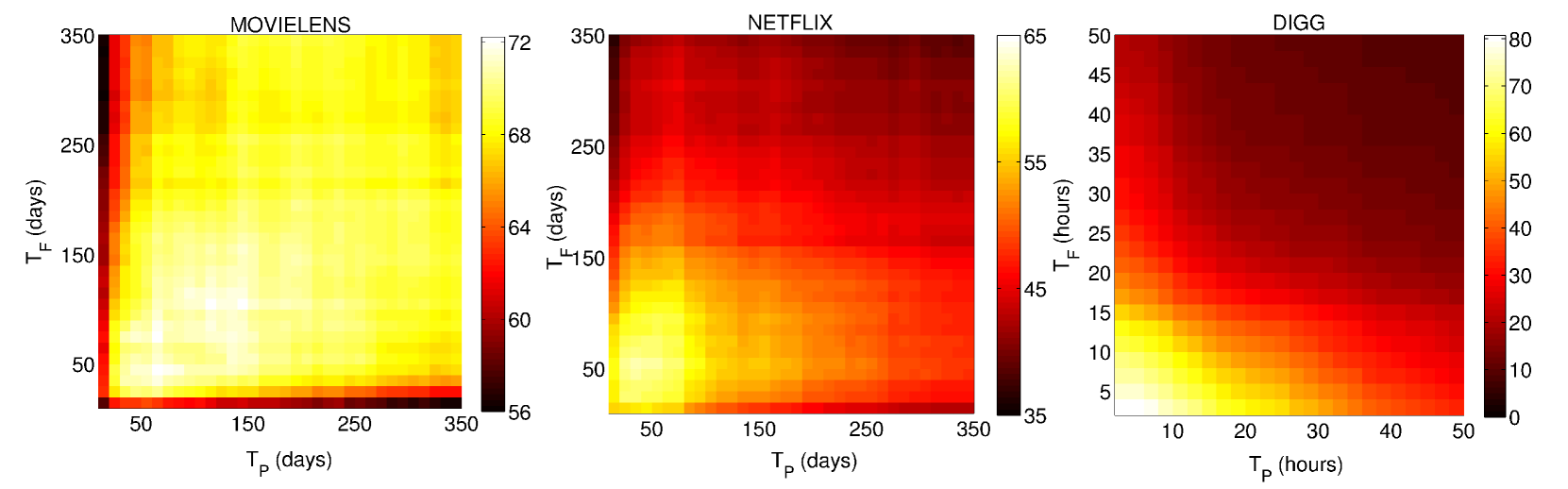
Figure 1: (Color online) Heat map of precision $P_{100}$ obtained with the degree increase predictor in the past/future time window plane $(T_{P},T_{F})$. Time is measured in days for Netflix and Movielens and in hours for Digg.

In the context of the Barabási-Albert model, the expected popularity increase of an item is proportional to the item’s degree and the two predictors, $\Delta k$ and $k$, are expected to produce rankings that are identical on average (though, $\Delta k$ is a more noisy indicator than $k$). As already mentioned, patterns in real data often substantially differ from the basic Barabási-Albert scenario and rankings produced by the two predictors are thus expected to diverge to some extent. To benefit from these two complementary sources of information, we introduce parameter $\lambda\in[0,1]$ which interpolates between them and introduce the hybrid item score in the form

$$s_{\alpha}(t^{*},T_{P})=k_{\alpha}(t^{*})-\lambda k_{\alpha}(t^{*}-T_{P}).$$ (2)

This simplifies to the total popularity (degree) for $\lambda=0$ and to the recent popularity (degree increase) for $\lambda=1$. We refer to this as the popularity-based predictor (PBP).

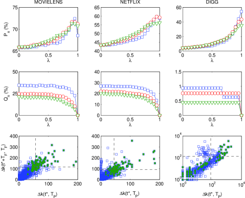
Figure 2: (Color online) Results for the PBP predictor defined by Eq. (2). $T_{F}$ is set to $90\,\mathrm{days}$ days for Movielens/Netflix and $10\,\mathrm{hours}$ for Digg in all simulations. Top row: Precision versus $\lambda$ for different past time windows $T_{P}$: blue lines with squares ($T_{P}=30\,\mathrm{days}$ in Netflix/Movielens and $T_{P}=10\,\mathrm{hours}$ in Digg), red lines with circles ($T_{P}=60\,\mathrm{days}$ in Netflix/Movielens and $T_{P}=20\,\mathrm{hours}$ in Digg), and green lines with triangles ($T_{P}=90\,\mathrm{days}$ in Netflix/Movielens and $T_{P}=30\,\mathrm{hours}$ in Digg). Middle row: Rate of correctly guessed new entries $Q_{n}$ versus $\lambda$ (different lines as in the top row). Bottom row: Scatter plots of item degree increase in $(t^{*}-T_{P},t^{*}]$ versus the degree increase in $(t^{*},t^{*}+T_{F}]$ with both history and future window lengths $60$ days for Netflix and Movielens and $10$ hours for Digg. Items placed by the PBP method with $\lambda=0.9$ in top 100 are marked with full green symbols.

Results obtained with PBP for different values of $\lambda$ are shown in Fig. 2. Recent popularity gives better results than total popularity in all datasets, especially in Digg where interest in a story fades quickly and the absolute popularity hence yields a particularly low precision value. For both Movielens and Netflix, there is an intermediate value of the parameter $\lambda$ outperforming both total and recent popularity. The optimal value of $\lambda$ is approximately $0.9$ in both cases. The absence of such a maximum in Digg confirms the intuition that the temporal evolution of news popularity substantially differs from that of movies. The rate of correctly predicted new items $Q_{n}$ monotonically decreases with $\lambda$ in both Movielens and Netflix and reaches $0$ for $\lambda=1$ (by definition because $\lambda=1$ corresponds to prediction by popularity increase where items with low recent popularity cannot score high). $Q_{n}$ values are very low in the case of Digg which is due to the quick dynamics of news which makes it nearly impossible that an old item with high degree can be among the top growing items in the near future. This is in line with Szabo2010 where high correlation has been found between popularity of stories early after their submission and their final popularity.

Fig. 2 further includes scatter plots showing popularity increase in the past and future time window for individual items (no averaging over $t^{*}$ was applied). The vertical dashed line marks the degree of the 100th most popular item in the history window and the horizontal dashed line marks the degree of the 100th most popular item in the future window. The top $100$ items predicted by PBP with $\lambda=0.9$ are marked with full symbols. The meaning of $C_{n}$ is well illustrated by these scatter plots. Among the top $100$ most popular items in the future time window, some were among the top $100$ most popular also in the past time window (the top-right quadrant in the scatter plots) and some are new—they were not among the top $100$ most popular in the past (the top-left quadrant). Items from the top-left quadrant are more difficult to be predicted and for this reason they are more valuable. By setting $\lambda<1$ in the PBP, the top $100$ predicted items cease to be located only in the top-right and bottom-right quadrant and some of them appear in our target top-left quadrant ($C_{n}$ is equal to the number of these items) as well as in the bottom-left quadrant (where they represent wrong predictions similarly as the predicted items located in the bottom-right quadrant). We can conclude that intermediate values of $\lambda$ highlight some of the items that are increasing their popularity at a faster pace than they did in the recent past. This is however not the case for Digg where the value of $Q_{n}$ stays virtually zero regardless of $\lambda$.

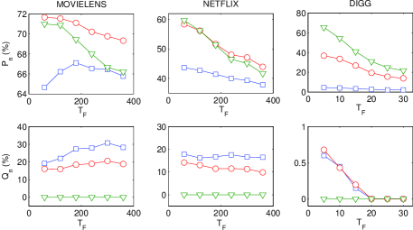
Figure 3: (Color online) Top row: Precision vs the future time window length $T_{F}$ for different values of $\lambda$: $\lambda=0$ (blue lines with squares), $\lambda=0.9$ (red lines with circles), and $\lambda=1$ (green lines with triangles). The past time window length is $T_{P}=2\,\mathrm{months}$ for Movielens/Netflix and $10\,\mathrm{hours}$ for Digg. Bottom row: Rate of correctly guessed new entries $Q_{n}$ as a function of the future time window length $T_{F}$ and different values of $\lambda$ (the same lines as in the top row).

We further investigate how the PBP method performs as a function of the future time window length $T_{F}$ for different values of $\lambda$. As can be seen in Fig. 3, predictions based on the popularity increase ($\lambda=1$ and $\lambda=0.9$) give better results than those based on total popularity ($\lambda=0$) but their performance decreases with $T_{F}$ faster than for $\lambda=1$ and $\lambda=0.9$. This confirms that total popularity is a reliable and stable predictor for the long run but it can be outperformed by other methods for short time windows. PBP with $\lambda=0.9$ gives on overall the best performance and is rather stable when the future time window is varied. In the case of Digg, it is always best to use pure popularity increase for prediction and, closely related, the decrease of precision of with $T_{F}$ is the steepest out of the three tested datasets.

II.2 Trend setters: a weighted popularity predictor

In the PBP method, all users are considered equal: only the number of users who have collected an item matters. It is however possible that some users are better than the others in detecting promising items and that their choice is only afterwards followed by other users who are more popularity-driven and less attentive to the emerging trends. However, Movielens and Netflix datasets lack any additional user information which could allow us to assess user weights. We thus have to base our judgment only on the rating activity of users which can be measured either as the number of recent ratings $\Delta k_{i}(t^{*},T_{P})$ or as the total number of ratings $k_{i}(t^{*})$. Since the total activity performs slightly better in our tests, we define the weighted popularity predictor (WPP) in the form

$$s_{\alpha}(t^{*},T_{P})=\sum_{i}\big{(}A_{i\alpha}(t^{*})-A_{i\alpha}(t^{*}-T_{P})\big{)}k_{i}(t^{*})^{\gamma}.$$ (3)

Here $\gamma$ is a tunable parameter which defines how much greater (when $\gamma>0$) or lower (when $\gamma<0$) weight is given to active users. When $\gamma=0$, the predicted score reduces to the popularity increase in the past time window. As can be seen in Fig. 4, prediction precision achieves a maximum around $\gamma=0$ in Movielens and Netflix. In Digg, positive values of $\gamma$ lead to a considerable increase in the precision value. Furthermore, both $\gamma>0$ and $\gamma<0$ allow us to achieve significant rates of correctly predicted new entries $Q_{n}$, which means that the method is able to detect promising items. This feature is most pronounced when $\gamma>0$ in Digg. Notably, approximately one third of these items are not found by the popularity-based predictor because their popularity on the test date $t^{*}$ is too small. As before, we make also scatter plots of the popularity increase (see Fig. 4) which further demonstrate the ability of the WPP to detect the emerging items and avoid those that fade away. The performance dependence on the future window length $T_{F}$ can be studied too and shows that when $T_{F}$ increases, activity-favoring predictions ($\gamma>0$) suffer less than activity-disfavoring ones ($\gamma<0$).

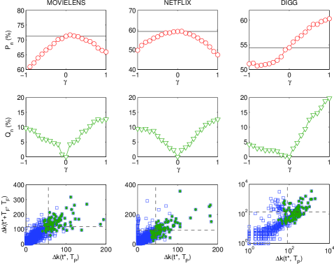
Figure 4: (Color online) Top row: Prediction precision versus $\gamma$ for WPP. Horizontal lines correspond to results obtained with the simple $\Delta k$ predictor. Middle row: The rate of correctly guessed new entries, $Q_{n}$ versus $\gamma$. Bottom row: Scatter plots of item degree increase in $(t^{*}-T_{P},t^{*}]$ versus the degree increase in $(t^{*},t^{*}+T_{F}]$. Full symbols correspond to items predicted by the WPP method. In all cases, both history and future window lengths are $60$ days for Netflix and Movielens and $10$ hours for Digg.

III Trend Prediction Augmented by User Centrality in the Social Network

We now focus on the Digg dataset for which, unlike the Movielens and Netflix data, we have also the social network of connections among the users. In the case of Digg, it is a directed leader-follower network thanks to which followers receive stories “dug” by their leaders. This social network contains 336,225 users and 2,251,171 links. The general idea is that prominent users in the social network can be more effective in propagating contents (because their reputation or their position in the social network boost the propagation of a story) or have better chances of digging promising contents (if their social status in the social network reflects their ability to filter good stories). The presence of influential users and their role in the propagation of information is still a controversial subject and it is not clear to which extent they can effectively influence the popularity of items or products WattsDuncanJandDodds2007 . This matter is also debated in the context of viral marketing Leskovec2007 ; Subramani2003 where it is not clear if large adoption of a product can be driven by a cascading word-of-mouth process. Our data is not detailed enough to allow us to see if prominent users (according to their number of followers or a more sophisticated centrality measure) are in fact directly responsible for propagation of stories. However, we can still assess if there is some benefit to be gained in our prediction task from user status in the social network.

We denote the adjacency matrix of the user social network as $\mathsf{G}$. $G_{ij}=1$ if user $i$ follows user $j$ and $0$ otherwise. Since the network is directed, matrix $\mathsf{G}$ is not necessarily symmetric and we distinguish between a node’s in-degree (number of followers) $d^{IN}_{i}=\sum_{j}G_{ji}$ and out-degree (number of leaders) $d^{OUT}_{i}=\sum_{j}G_{ij}$. For computational reasons we do not take into account the time dependence of the adjacency matrix $\mathsf{G}$ in the social network. We denote the influence of user $i$ as $I_{i}$ (we specify it later) and compute the influence-based predictor (IBP) similarly as in Eq. (3), that is by weighting the contribution of each user by this user’s influence

$$s_{\alpha}(t^{*},T_{P})=\sum_{i}\big{(}A_{i\alpha}(t^{*})-A_{i\alpha}(t^{*}-T_{P})\big{)}I_{i}^{\eta}.$$ (4)

Parameter $\eta$ makes it possible to tune the contribution of user influence (when $\eta=0$, the method simplifies to the original influence-free popularity increase).

We are free to choose from various influence measures (in social sciences, the term centrality metric is often used instead Bonacich1987 ). The simplest measure of influence is the user in-degree (the number of followers), in which case we simply set $I_{i}=d^{IN}_{i}$ and call the corresponding predictor IBP-IN. As more refined measures of influence, we choose the PageRank Page1999 and the LeaderRank Lu2011 , giving rise to two predictors: IBP-PR and IBP-LR, respectively. Both PageRank and LeaderRank are reputation metrics which derive the influence of a user from the influence of his followers in a self-consistent way. These two methods are shown to outperform the in-degree in identifying the influential users for spreading Lu2011 . In both algorithms, users are first initialized with the same score. The PageRank score of a user is then computed by iterating a process where a fraction $\delta\in(0,1)$ of the score of a user is transferred in equal shares to its leaders (we set $\delta=0.85$ as in the original paper). The remaining $1-\delta$ fraction of the score is evenly redistributed to all users in the network. The LeaderRank score is computed in a similar way with the difference that $\delta$ is set to $1$ and a ground node is introduced and connected with all user nodes by bidirectional links. This algorithm is parameter-free and it is based on the assumption that users with few leaders owe a larger share of their reputation to the entire community than users with many leaders.

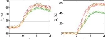
Figure 5: (Color online) Prediction precision $P_{n}$ and the rate of correctly guessed new entries $Q_{n}$ versus $\eta$ in Digg for different user centrality measures: number of followers (IBP-IN, red lines with circles), PageRank (IBP-PR, green lines with triangles), and LeaderRank (IBP-LR, orange lines with diamonds). Horizontal lines correspond to the results obtained with the simple $\Delta k$ predictor.

Past work on predicting future popularity of Digg content focuses on individual stories Szabo2010 and predictions of the top-$L$ most popular items haven’t been studied yet. We can thus only present the results obtained with the simple $\Delta k$ predictor as comparison. As one can see in Fig. 5, all three measures of influence yield significantly higher precision than the bare popularity increase and the rate of correctly predicted new items is also considerably higher than, for example, in Fig. 4. Although we cannot draw any causal implications from this observation, we can say that measures of social influence importantly enhance the performance of future popularity increase predictions. Performance obtained with PageRank or LeaderRank weighting is better (with respect to both $P_{n}$ and $Q_{n}$) than that obtained with bare in-degree, confirming the added value of these two centrality measures. Note that in the Digg dataset, a large part of these correctly guessed new entries $Q_{n}$ cannot be predicted neither by their recent popularity increase (by definition) nor by their total popularity. This means that the IBP method is able to find inherently unexpected items whose upcoming popularity is due to the social processes taking place in the system. Similar results follow when top $n=50$ and $n=200$ places of rankings are evaluated.

IV Conclusions

We investigated the ability of different methods to predict which items are going to have the biggest popularity increase in the near future. When items in the studied system have short typical lifetime (which, for example, is the case for the Digg data studied herein), predictions by total popularity result in poor performance while predictions by recent popularity perform well. In Netflix and Movielens data we find that recent popularity is a good predictor for short future time windows but its performance decreases fast with the future window length. Predictions by total popularity, instead, are more stable in this sense and perform reasonably well also in the long run. By combining these two predictors, one can achieve a slightly higher precision and a large increase in the number of correctly guessed items that are new at the top of the ranking. We found in all studied datasets that weighted popularity increase which takes user activity into account, while not so useful for improving the prediction precision, can detect items whose popularity was not particularly high in the recent past. Finally, in the case of the Digg data we found that knowledge of the underlying user social network can significantly enhance the prediction results. To achieve this improvement, we weighted users with various measures of social status (in-degree, PageRank, and LeaderRank) and found that both precision and the ability to predict items that were recently not so popular improve. In summary, the hybrid method combining the total item popularity with recent popularity allows for some improvements in the case of Netflix and Movielens. In Digg, the benefit gained from the knowledge of the social network among the users is substantial and the weighted predictor based on social influence achieves improvements in accuracy and, even more, in the ability to correctly predict new items at top places of the ranking.

Our study is an exploratory one and there is much work that remains to be done in the future. First of all, to test the methods on more datasets would be useful to show possible limits of their applicability. One should also invest the computational effort to evaluate the methods on large-scale data—both for the sake of confirming previously found patterns and for evaluating which computation steps can be simplified. For practical applications of the ideas proposed in this work, it would be very important to devise scalable algorithms able to cope with the massive data routinely produced by the current online systems. For large-scale data, one can also devise methods that benefit from the often-available additional information such as user and item meta data. Robust statistical techniques could reveal that, for example, users with certain background (say, females under 25 years) are particularly significant for predicting popularity of a specific kind of contents. How much this could improve the predictions is of course an open question.

Besides devising further techniques for trend prediction, we find it important to search for additional metrics to assess the prediction performance. For example, incorporating the order of the ranking will increase the information of the prediction. Moreover, it would be interesting to focus on items which are in the early stage of their evolution—one can say that the ability to predict success of those would be of foremost usefulness to the users. Our metric $Q_{n}$ makes a step in this direction by counting the items which are new in the top-$100$ ranking of items by their recent popularity. However, it does not account for the fact that some of those “new” items can already have substantial total popularity and they only return to the group of recently popular items after a momentous lapse. The natural way to aim for those well-performing new items is to define the logarithmic derivative of the popularity, $\Delta k/k$, as the true score and see how to predict this ranking. However, we found it difficult to work with $\Delta k/k$ because of the excess weight that it puts on low-degree items (highest values are achieved by items with very low $k$) and the resulting sensitivity to the discreteness of time in the data. For example, an item submitted short before midnight accumulates only a few links on the first day and then excels—to some extent without reason—in $\Delta k/k$ the day after. Devising more reliable and justifiable metrics focusing on genuinely new items thus remains a future challenge.

References

- (1) Ahn, Y.-Y., Han, S., Kwak, H., Moon, S., and Jeong, H., Analysis of topological characteristics of huge online social networking services, in Proceedings of the 16th international conference on World Wide Web - WWW ’07 (ACM Press, New York, New York, USA, 2007), p. 835, doi:10.1145/1242572.1242685.
- (2) Barabási, A.-L. and Albert, R., Emergence of Scaling in Random Networks, Science 286 (1999) 509–512.
- (3) Bollen, J., Mao, H., and Zeng, X.-J., Twitter mood predicts the stock market, Computer 2 (2010) 1–8.
- (4) Bonacich, P., Power and Centrality: a Family of Measures, JSTOR: American Journal of Sociology 92 (1987) 1170—-1182.
- (5) Crane, R. and Sornette, D., Robust dynamic classes revealed by measuring the response function of a social system., Proceedings of the National Academy of Sciences of the United States of America 105 (2008) 15649–53.
- (6) Deng, H., Lyu, M. R., and King, I., A generalized co-hits algorithm and its application to bipartite graphs, in Proceedings of the 15th ACM SIGKDD international conference on Knowledge discovery and data mining, KDD ’09 (ACM, New York, NY, USA, 2009), pp. 239–248, doi:10.1145/1557019.1557051.
- (7) Ding, Y., Li, X., and Orlowska, M. E., Recency-based collaborative filtering, in Proceedings of the 17th Australasian Database Conference - ADC ’06 (ACM Press, 2006), pp. 99–107.
- (8) Herlocker, J. L., Konstan, J. A., Terveen, L. G., and Riedl, J. T., Evaluating collaborative filtering recommender systems, ACM Transactions on Information Systems 22 (2004) 5–53.
- (9) Holme, P. and Saramäki, J., Temporal networks, Physics Reports 519 (2012) 97–125.
- (10) Huberman, B. A., Romero, D. M., and Wu, F., Social networks that matter: Twitter under the microscope, SSRN Electronic Journal (2008).
- (11) Jamali, S. and Rangwala, H., Digging Digg: Comment Mining, Popularity Prediction, and Social Network Analysis, in 2009 International Conference on Web Information Systems and Mining (IEEE, 2009), pp. 32–38, doi:10.1109/WISM.2009.15.
- (12) Kempe, D., Kleinberg, J., and Tardos, E., Maximizing the spread of influence through a social network, in Proceedings of the ninth ACM SIGKDD international conference on Knowledge discovery and data mining - KDD ’03 (ACM Press, New York, New York, USA, 2003), p. 137, doi:10.1145/956750.956769.
- (13) Kumar, R., Novak, J., and Tomkins, A., Structure and Evolution of Online Social Networks, in Link Mining: Models, Algorithms, and Applications, eds. Yu, P. S. S., Han, J., and Faloutsos, C. (Springer New York, 2010), pp. 337–357.
- (14) Lerman, K. and Ghosh, R., Information contagion: an empirical study of spread of news on digg and twitter social networks, in Proceedings of 4th International Conference on Weblogs and Social Media - ICWSM ’10 (Association for the Advancement of Artificial Intelligence, 2010), pp. 90–97.
- (15) Lerman, K. and Hogg, T., Using a model of social dynamics to predict popularity of news, in Proceedings of the 19th international conference on World wide web - WWW ’10 (ACM Press, New York, New York, USA, 2010), p. 621, doi:10.1145/1772690.1772754.
- (16) Leskovec, J., Adamic, L. A., and Huberman, B. A., The dynamics of viral marketing, ACM Transactions on the Web 1 (2007) 5–es.
- (17) Leskovec, J., Backstrom, L., Kumar, R., and Tomkins, A., Microscopic evolution of social networks, in Proceeding of the 14th ACM SIGKDD international conference on Knowledge discovery and data mining - KDD ’08 (ACM Press, New York, New York, USA, 2008), p. 462, doi:10.1145/1401890.1401948.
- (18) Lü, L., Zhang, Y.-C., Yeung, C. H., and Zhou, T., Leaders in social networks, the Delicious case., PloS one 6 (2011) e21202.
- (19) Medo, M., Cimini, G., and Gualdi, S., Temporal Effects in the Growth of Networks, Physical Review Letters 107 (2011).
- (20) Mislove, A., Marcon, M., Gummadi, K. P., Druschel, P., and Bhattacharjee, B., Measurement and analysis of online social networks, in Proceedings of the 7th ACM SIGCOMM conference on Internet measurement - IMC ’07 (ACM Press, New York, New York, USA, 2007), p. 29, doi:10.1145/1298306.1298311.
- (21) Page, L., Brin, S., Motwani, R., and Winograd, T., The PageRank Citation Ranking: Bringing Order to the Web. (1999).
- (22) Price, D. D. S., A general theory of bibliometric and other cumulative advantage processes, Journal of the American Society for Information Science 27 (1976) 292–306.
- (23) Robins, G. and Alexander, M., Small Worlds Among Interlocking Directors: Network Structure and Distance in Bipartite Graphs, Computational & Mathematical Organization Theory 10 (2004) 69–94.
- (24) Subramani, M. R. and Rajagopalan, B., Knowledge-sharing and influence in online social networks via viral marketing, Communications of the ACM 46 (2003) 300.
- (25) Szabo, G. and Huberman, B. A., Predicting the popularity of online content, Commun. ACM 53 (2010) 80–88.
- (26) Tsagkias, M., Weerkamp, W., and de Rijke, M., Predicting the volume of comments on online news stories, in Proceeding of the 18th ACM conference on Information and knowledge management - CIKM ’09 (ACM Press, New York, New York, USA, 2009), p. 1765, doi:10.1145/1645953.1646225.
- (27) Walker, D., Xie, H., Yan, K.-K., and Maslov, S., Ranking scientific publications using a model of network traffic, Journal of Statistical Mechanics: Theory and Experiment (2007) P06010.
- (28) Watts, D. J. and Dodds, P. S., Influentials, Networks, and Public Opinion Formation, JSTOR: Journal of Consumer Research 34 (2007) 441—-458.
- (29) Yang, J. and Leskovec, J., Patterns of temporal variation in online media, in Proceedings of the fourth ACM international conference on Web search and data mining - WSDM ’11 (ACM Press, New York, New York, USA, 2011), p. 177, doi:10.1145/1935826.1935863.
- (30) Yule, G. U., A Mathematical Theory of Evolution, Based on the Conclusions of Dr. J. C. Willis, F.R.S., Philosophical Transactions of the Royal Society of London. Series B, Containing Papers of a Biological Character 213 (1925) pp. 21–87.
- (31) Zhou, T., Ren, J., Medo, M., and Zhang, Y.-C., Bipartite network projection and personal recommendation, Phys. Rev. E 76 (2007) 46115.