Bayesian analysis of measurement error models using INLA

Abstract

To account for Measurement error (ME) in explanatory variables, Bayesian approaches provide a flexible framework, as expert knowledge about unobserved covariates can be incorporated in the prior distributions. However, given the analytic intractability of the posterior distribution, model inference so far has to be performed via time-consuming and complex Markov chain Monte Carlo implementations. In this paper we extend the Integrated nested Laplace approximations (INLA) approach to formulate Gaussian ME models in generalized linear mixed models. We present three applications, and show how parameter estimates are obtained for common ME models, such as the classical and Berkson error model including heteroscedastic variances. To illustrate the practical feasibility, R-code is provided.

Leonhard Held, Division of Biostatistics, Institute of Social and Preventive Medicine, University of Zurich, Hirschengraben 84, 8001 Zurich, Switzerland.

1 Introduction

The existence and the effects of measurement error (ME) in statistical analyses have been recognized and discussed for more than a century, see for example Pearson (1902); Wald (1940); Berkson (1950); Fuller (1987); Carroll et al. (2006). The sources of ME are manifold and imply much more than just instrumental imprecision in the measurement of physical variables, such as length, weight etc., but may include for instance biases due to preferential sampling, incomplete observations or misclassification.

If ME is ignored, parameter estimates and confidence intervals in statistical models often suffer from serious biases. If a regression model is multivariate and some covariates can be measured with and some without error, even the effects of the error-free measured covariates can be biased, where the direction of the bias depends on the correlation among covariates (Carroll et al., 1985; Gleser et al., 1987). Moreover, ME may cause a loss of power for detecting signals and connections among variables, and may mask important features of the data. Given these facts, it is surprising that ME is often completely ignored or not treated properly. One reason might be that standard statistical textbooks on regression often pay very little attention to this aspect, although the problems have been recognized for a long time.

For successful error-correction both the amount of error (i.e. the error variance) and the error model need to be specified correctly. Hence, information about the underlying measurement process is essential. Possible errors must be identified early in a study and the entire data-collection process should be driven by such considerations. In the last decades, several approaches to model and correct for ME have been proposed, such as method-of-moments corrections (Fuller, 1987), simulation extrapolation (SIMEX) (Cook and Stefanski, 1994), regression calibration (Carroll and Stefanski, 1990; Gleser, 1990), or Bayesian analyses (Clayton, 1992; Stephens and Dellaportas, 1992; Richardson and Gilks, 1993; Dellaportas and Stephens, 1995; Gustafson, 2004). A thorough overview of current state-of-the-art methods is given in the books of Carroll et al. (2006) and Buonaccorsi (2010).

In this paper, we focus on Bayesian approaches where prior knowledge, and in particular prior uncertainty, e.g., in variance estimates, can be incorporated in the model. Up to now, posterior marginal distributions in such measurement error models have been estimated by employing a Markov chain Monte Carlo (MCMC) sampler, see for example Stephens and Dellaportas (1992) or Richardson and Gilks (1993). However, case-specific implementation may be challenging, MCMC is time-consuming, and its analysis and interpretation requires diagnostic tools. Generic software like WinBugs (Lunn et al., 2000), OpenBugs (Lunn et al., 2009), or MCMC samplers in R, such as MCMCpack (Martin et al., 2011), might be used, but they suffer from the same drawbacks as any MCMC technique.

Recently, an alternative to MCMC has been proposed to estimate posterior marginals by integrated nested Laplace approximations (INLA) for the class of latent Gaussian models (Rue et al., 2009). INLA provides accurate approximations avoiding time-consuming sampling. Due to its flexibility in the choice of likelihood functions and latent models, INLA is an appealing alternative to likelihood-based inference in particular for generalized linear mixed models (GLMMs) (Fong et al., 2010). The INLA approach is implemented in C and easy to use under Linux, Windows and Macintosh via a freely available R-interface (R Core Team, 2012). The R-package r-inla can be downloaded from www.r-inla.org. Using this package models can be specified in a modular way, where different types of regression models can be combined with different types of error models. Moreover, it is straightforward to incorporate random effects, such as independent or conditional autoregressive (CAR) models to account for spatial structure, which is of importance in several settings (Bernardinelli et al., 1997). Here, we used the r-inla version updated on July 13, 2013.

In this paper we extend the INLA framework to the most common Gaussian ME models, namely the classical and the Berkson ME models, which are suitable for continuous error-prone covariates. To facilitate the usage of the INLA-package with the new features, R-code is provided in the Supplementary Material. We hope that the solution presented here will increase the use of ME thinking in practice and stimulates the greater use of Bayesian methods in ME modelling.

Section 2 introduces three applications from the biological/medical field containing: a linear regression combined with heteroscedastic classical error, a logistic model with an binary error-free covariate and one suffering from classical error, and an overdispersed Poisson regression model with Berkson error. In Section 3 we will review the classical and Berkson ME models and their effects. Bayesian analysis with INLA is introduced in Section 4, where we will describe how to use this framework for model inference in the presence of classical and Berkson ME. Section 5 presents modelling details and the results of the three applications analyzed with both INLA and MCMC. Finally, we provide a discussion and outlook in Section 6.

2 Examples of measurement error problems

In this Section we introduce three applications which will be discussed in more detail in Section 5. Here, we mainly describe the problem at hand and the difference of the results depending on whether or not measurement error has been incorporated in the analysis. All parameter estimates in measurement error models are obtained using INLA, as described in detail in subsequent sections.

2.1 Inbreeding in Swiss ibex populations

We analyzed data described by Bozzuto et al. (2013) on $26$ Alpine ibex populations in Switzerland, some of them monitored over the past 100 years. The study aimed to quantify the effect of inbreeding on populations’ intrinsic growth rates. The intrinsic growth rate $y_{i}$ of a population $i$ is the theoretical maximal rate of increase, if there are no density-dependent effects. The inbreeding coefficient ${x_{i}}$ of population $i$ (often denoted as $f_{i}$) is a quantity between $0$ and $1$, with larger values indicating stronger inbreeding. Unfortunately, $x_{i}$ cannot be measured exactly. A Bayesian analysis based on genotype experiments at $37$ neutral microsatellite loci was employed to derive estimates for $x_{i}$, denoted by $w_{i}$, which additionally provided error variances for each population $i$. Additional covariates that may influence the intrinsic growth rate include the number of years a population was observed, the average precipitation in summer, an interaction between the two, and the average precipitation in winter. These covariates are treated as error-free and subsumed in a row vector $\bm{z}_{i}$.

Fitting a linear regression model $\operatorname{\mathsf{E}}({y}_{i})=\beta_{0}+\beta_{x}x_{i}+\bm{z}_{i}\bm{\beta_{z}}$ in INLA using the proxy $w_{i}$ instead of the true but unobserved ${x}_{i}$, the absolute value of the slope parameter $|\beta_{x}|$ is underestimated ($\hat{\beta}_{x}=-0.91$, 95% CI: $[-2.17,0.36]$). Indeed, after accounting for ME the effect of inbreeding on population growth dynamics is more pronounced ($\hat{\beta}_{x}=-1.84$, 95% CI: $[-3.88,0.11]$).

2.2 Influence of systolic blood pressure on coronary heart disease

The Framingham heart study is a large cohort study that aimed to understand the factors leading to coronary heart disease and, in particular, characterize the relation to systolic blood pressure (SBP) (Kannel et al., 1986). The outcome ${y}_{i}\in\{0,1\}$ is a binary indicator for presence of the disease, and modelled via a logistic regression. We analysed data from $n=641$ males originally presented in MacMahon et al. (1990). As in Carroll et al. (2006, Section 9.10), we use $x_{i}=\log(\text{SBP}_{i}-50)$ and a binary smoking status indicator $z_{i}\in\{0,1\}$ as predictors. The transformation of SBP, originally proposed by Cornfield (1962), has also been used in Carroll et al. (1984, 1996, 2006). Since it is impossible to measure the long-term SBP, measurements at single clinical visits had to be used as a proxy. Note that, due to daily variations or deviations in the measurement instrument, the single-visit measures might considerably differ from the long-term blood pressure (Carroll et al., 2006). Hence, the ME in SBP has been a concern for many years in this study. Importantly, the magnitude of the error could be estimated, as SBP had been measured twice at different examinations. These proxy measures for $x_{i}$ are denoted as $w_{1i}$ and $w_{2i}$. A naive approach ignoring ME would fit a logistic regression against the indicator of coronary heart disease

$$\text{logit}\left[\operatorname{\mathsf{Pr}}({y}_{i}=1)\right]=\beta_{0}+\beta_{x}{x}_{i}+\beta_{z}z_{i}\ ,$$

where the true covariate ${x}_{i}$ is replaced by the centered mean of the two (suitably transformed) SBP measurements. The slope $\beta_{x}$ is attenuated in this naive regression ($\hat{\beta}_{x}=1.66$, 95% CI: $[0.70,2.63]$) compared to the estimate obtained with error modelling ($\hat{\beta}_{x}=1.89$, 95% CI: $[0.80,3.00]$).

2.3 Seedling growth across different light conditions

The impact of shading (dark, middle, light) and defoliation ($0\%$, $25\%$, $50\%$, $75\%$ reduction of leaf surface) on plant seedling growth in the Malaysian rainforest has been investigated in a planned experiment described in Paine et al. (2012). The number of new leaves per plant after a four months growth phase was counted and used as the response variable for plant growth. Here, we analyzed $60$ seedlings from the species Shorea fallax, from which $20$ plants were grown each under dark, middle, and light shading conditions. There were five shadehouses for each of the three shading conditions, and each shadehouse contained four seedlings. Each seedling in a shadehouse was exposed to a different degree of defoliation treatment, compare Figure 1. In experimental studies in ecology, it is common practice that the value for the target light intensity $\bm{w}$ (given in % and transformed to the log-scale) is assigned to all replicates within a treatment class (i.e. dark, middle, light). However, due to external conditions the actual observed light availability $\bm{x}$ might considerably vary from the target value within replicates. Therefore, the target light intensity takes only three different values (one for dark, middle and light), while the actual light availability would take 15 different values (one for each shadehouse).

The selected regression model is Poisson with (log) target light intensity as proxy for the actual observed light availability, and additional unstructured random effects to account for potential overdispersion. In contrast to the preceding examples 2.1 and 2.2, where the inclusion of $\bm{w}$ instead of $\bm{x}$ in the regression attenuates the parameter estimates, theory for log-linear models with Berkson error suggests that there is no bias in the regression coefficients (Carroll, 1989). However, it is not clear if this result extends to models with random effects. Our analysis did not reveal a difference in the regression coefficients after accounting for measurement error. We did observe a slightly increased credible interval width for the regression coefficients, and, in particular, for the precision of the random effects.

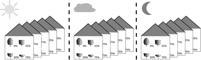
Figure 1: Illustration of the shadehouse experiment. There were five shadehouses per light condition and each shadehouse contained four seedlings. The seedlings in a shadehouse were each exposed to a different defoliation treatment, 0% indicating that the leaves were not cut, 25% that one fourth of each leaf was cut, etc.

3 Measurement error models in regression

3.1 The generalized linear model

Assume we have $n$ observations in a generalized linear model (GLM). The data are given as $(\bm{y},\bm{z},\bm{x})$, with $\bm{y}=(y_{1},\ldots,y_{n})^{\top}$ denoting the response, $\bm{z}=(\bm{z}_{1},\ldots,\bm{z}_{p})$ a covariate matrix of dimension $n\times p$ for $p$ error-free covariates, and $\bm{x}=({x}_{1},\ldots,{x}_{n})^{\top}$ a single error-prone covariate whose true values are unobservable. The generalization to multiple error-prone covariates is straightforward. Suppose $\bm{y}$ is of exponential family form with mean $\mu_{i}=\operatorname{\mathsf{E}}(y_{i}\,|\,\bm{x},\bm{z},\bm{\beta})$, linked to the linear predictor $\eta_{i}$ via

$$\mu_{i} =h(\eta_{i})$$

$$\eta_{i} =\beta_{0}+\beta_{x}x_{i}+\bm{z}_{[i,]}\bm{\beta}_{z}\ .$$ (1)

Here, $h(\cdot)$ is a known monotonic inverse link (or response) function, $\beta_{0}$ denotes the intercept, $\beta_{x}$ the fixed effect for the error-prone covariate $\bm{x}$, and $\bm{z}_{[i,]}$ is $1\times p$ with a corresponding vector $\bm{\beta}_{z}$ of fixed effects. This GLM is extended to a generalized linear mixed model (GLMM) by adding normally distributed random effects on the linear predictor scale (1).

Let $\bm{w}=(w_{1},\ldots,w_{n})^{\top}$ denote the observed version of the true, but unobserved covariate $\bm{x}$. We distinguish two different ME processes: the classical error model and the Berkson error model (Berkson, 1950). The graphical structure of these models is very similar, compare Figure 2, but the caused effects are fundamentally different.

3.2 Classical measurement error model

In the classical error model it is assumed that the covariate $\bm{x}$ can be observed only via a proxy $\bm{w}$, such that, in vector notation,

$$\bm{w}=\bm{x}+\bm{u}\ ,$$

with $\bm{u}=(u_{1},\ldots,u_{n})^{\top}$. Throughout the paper the components of the error vector $\bm{u}$ are assumed to be independent and normally distributed with mean zero and variance $\tau_{u}^{-1}$, i.e. $\text{Cov}(u_{i},u_{j})=0$ for $i\neq j$. Note that in the following we parameterize the normal distribution with mean and precision (or precision matrix in the multivariate context), rather than using the variance or covariance matrix.

We assume that the error term $\bm{u}$ is independent of the true covariate $\bm{x}$, but also independent of any other covariates $\bm{z}$ and the response $\bm{y}$. This implies a non-differential ME model, meaning that $\bm{y}$ and $\bm{w}$ are conditionally independent given $\bm{z}$ and $\bm{x}$. In most applications this assumption is plausible as it implies that, given the true covariate $\bm{x}$ and covariates $\bm{z}$, no additional information about the response variable $\bm{y}$ is gained through $\bm{w}$ (Carroll et al., 2006). Ideally, repeated measurements $w_{ji}$, $j=1,\ldots,J$, of the true value $x_{i}$ are available, so that

$${w_{ji}}\,|\,{x_{i}}\sim\mathcal{N}({x_{i}},\tau_{u})\ .$$ (2)

More generally, the error structure can be heteroscedastic with $\bm{w}_{j}\sim\mathcal{N}(\bm{x},\tau_{u}\mathbf{D})$, where $\bm{w}_{j}$ denotes the vector of the $j^{th}$ measurements, and the entries in the diagonal matrix $\mathbf{D}$ represent weights $d_{i}$ that are proportional to the individual error precision $\tau_{u}(x_{i})$ depending on $x_{i}$, which allows for a heteroscedastic error structure. This is required when the accuracy of surrogate $w_{i}$ depends on $i$, i.e., $x_{i}$ can be measured with varying accuracy for different $i$. In fact, both the homo- and heteroscedastic cases are relevant in practice (see, e.g., Subar et al. (2001) or example 5.1 presented here).

Estimates of $\beta_{x}$ are usually attenuated in the classical ME setting if $\bm{w}$ is taken as a proxy for $\bm{x}$. Consider for instance a simple linear regression with homoscedastic ME. Fitting the naive model $\bm{y}=\beta_{0}^{\star}\bm{1}+\beta_{x}^{\star}\bm{w}+\bm{\varepsilon}^{\star}$ instead of the true model $\bm{y}=\beta_{0}\bm{1}+\beta_{x}\bm{x}+\bm{\varepsilon}$ will result in $|\beta_{x}^{\star}|<|\beta_{x}|$, if the error variance $1/\tau_{u}$ is larger than zero. The left panel of Figure 3 illustrates this attenuation affect. Another important effect is the significant increase of the variability around the regression line.

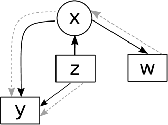
Figure 2: Graphical structure of the error models. Rectangular boxes illustrate variables that are observed, while circles indicate unknown variables. Black arrows correspond to the classical, and the dashed grey arrows to the Berkson error model. Note the change in direction of the arrow between $\bm{x}$ and $\bm{w}$.

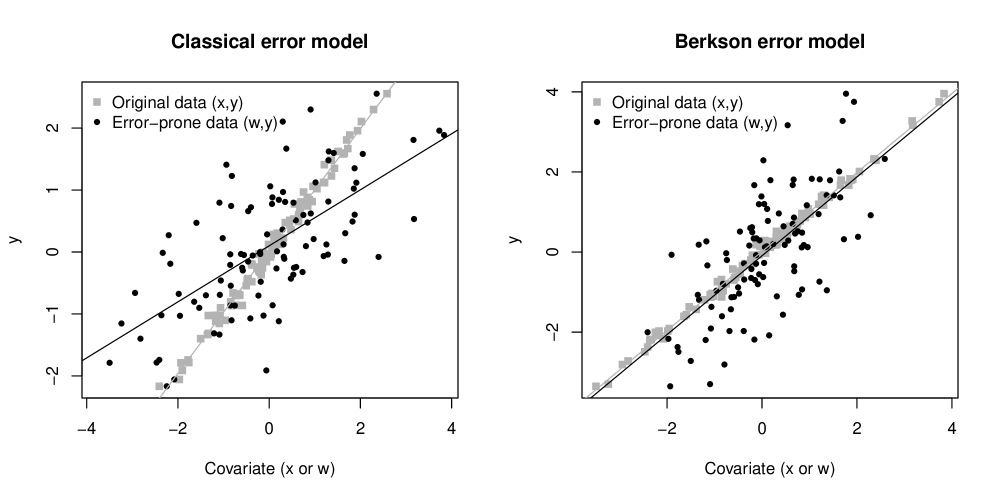
Figure 3: Effect of ME in the linear model. Left: Classical ME. Two effects can be seen: 1) The absolute value of the covariate estimate is biased (attenuated); 2) The variability around the regression line in the data with ME (black circles) is much larger than in the case of the truly observed data (grey squares). Right: Berkson ME. The absolute value of the covariate estimate is unbiased in the linear model, while the variability around the regression line is larger for the data with ME.

3.3 Berkson measurement error model

Berkson-type error can be observed in experimental settings, where the value of a covariate may correspond to, e.g., a predefined fixed dose, temperature or time interval, but the true values $\bm{x}$ may deviate from these planned values $\bm{w}$ due to imprecision in the realization. The second setting where Berkson-type error occurs is in epidemiological or biological studies, where, e.g., averages of exposures in areas are assigned to individuals living or working close-by. Examples are the application of fixed doses of herbicides in bioassay experiments (Rudemo et al., 1989) or the radiation epidemiology study described in Kerber et al. (1993) and Simon et al. (1995). Such circumstances led to the Berkson error model (Berkson, 1950)

$$\bm{x}=\bm{w}+\bm{u}\ ,$$

where $\bm{u}$ and $\bm{w}$ are independent, and

$$\bm{x}\,|\,\bm{w}\sim\mathcal{N}(\bm{w},\tau_{u}\mathbf{D})\ ,$$ (3)

with $\mathbf{D}$ denoting a diagonal matrix as in Section 3.2. Like classical ME, the Berkson error is also assumed to be non-differential. The effect of Berkson error is fundamentally different from that of classical error. In the linear regression model there is no attenuation effect, as illustrated in the right panel of Figure 3. However, the residual precision suffers from the same qualitative bias as in the classical ME model. Issues become more involved for GL(M)Ms. For instance, parameter estimates for logistic regression are only approximately consistent in the Berkson case (Burr, 1988; Bateson and Wright, 2010), which makes error modelling essential.

The difference between the classical and the Berkson error model is reflected in the relationships between the error variances. Denote with $\tau_{x}^{-1}$ and $\tau_{w}^{-1}$ the variances of $\bm{x}$ and $\bm{w}$, respectively. Due to the independence assumption of $\bm{x}$ and $\bm{u}$ in the classical and between $\bm{w}$ and $\bm{u}$ in the Berkson error case, the variances in the two ME models can be written as

$$\tau_{w}^{-1} = \tau_{x}^{-1}+\tau_{u}^{-1}\quad\text{(classical)}\ ,$$

$$\tau_{x}^{-1} = \tau_{w}^{-1}+\tau_{u}^{-1}\quad\text{(Berkson)}\ .$$

Thus, the surrogate $\bm{w}$ is more variable than the true covariate $\bm{x}$ in the classical model, whereas the opposite is true in the Berkson case. This effect can also be observed in Figure 3.

4 Analysis of measurement error models using INLA

A Bayesian analysis of ME models dates back to the seminal work of Clayton (1992) and is based on a three-level hierarchical model. The first level represents the observation model $\bm{y}\,|\,\bm{v},\bm{\theta}_{1}$ defining distributional assumptions about the response variable $\bm{y}$ in dependence on some unknown (latent) parameters $\bm{v}$ and certain hyperparameters $\bm{\theta}_{1}$, e.g. variance or correlation parameters. The second level describes the latent model or unobserved process $\bm{v}\,|\,\bm{\theta}_{2}$ depending on hyperparameters $\bm{\theta}_{2}$. In the third level, hyperpriors are defined for the hyperparameters $\bm{\theta}=(\bm{\theta}_{1}^{\top},\bm{\theta}^{\top}_{2})^{\top}$. The posterior distribution of $\bm{v}$ and $\bm{\theta}$ is then given by

$$\operatorname{{p}}(\bm{v},\bm{\theta}\,|\,\bm{y})\propto\operatorname{{p}}(\bm{y}\,|\,\bm{v},\bm{\theta})\operatorname{{p}}(\bm{v}\,|\,\bm{\theta})\operatorname{{p}}(\bm{\theta}).$$ (4)

Of primary interest are often the posterior marginal distributions of components $v_{i}$ of $\bm{v}$, which can be derived from (4) via

$$\operatorname{{p}}(v_{i}\,|\,\bm{y}) =\int_{\bm{\theta}}\int_{\bm{v}_{-i}}\operatorname{{p}}(\bm{v},\bm{\theta}\,|\,\bm{y})d\bm{v}_{-i}d\bm{\theta}\ ,$$ (5)

as well as posterior marginals of the hyperparameters $\theta_{j}$. The computation of massively high integrals is however very difficult. Except for cases where everything can be computed analytically, exact inference is challenging. Hence, sampling-based approaches have been the standard tool (Gelfand and Smith, 1990). Currently, few generic software packages based on MCMC, e.g. OpenBugs (Lunn et al., 2009), are available. However, MCMC based approaches are time-consuming and require diagnostic checks to ensure good mixing properties and convergence of the simulated samples.

Rue et al. (2009) proposed with INLA an efficient computing methodology based on accurate approximations to perform Bayesian inference in a sub-class of hierarchical models, namely latent Gaussian models. In this class the second level, the latent model, is assumed to be Gaussian. In the following we will shortly present the general idea of INLA.

INLA uses the fact that Equation (5) can also be written as

$$\operatorname{{p}}(v_{i}\,|\,\bm{y}) =\int_{\bm{\theta}}\operatorname{{p}}(v_{i}\,|\,\bm{\theta},\bm{y})\operatorname{{p}}(\bm{\theta}\,|\,\bm{y})d\bm{\theta}\ ,$$

and approximates this term by the finite sum

$$\tilde{\operatorname{{p}}}(v_{i}\,|\,\bm{y}) =\sum_{k}\tilde{\operatorname{{p}}}(v_{i}\,|\,\bm{\theta}_{k},\bm{y})\tilde{\operatorname{{p}}}(\bm{\theta}_{k}\,|\,\bm{y})\Delta_{k}\ .$$

Here, $\tilde{\operatorname{{p}}}(v_{i}\,|\,\bm{\theta},\bm{y})$ and $\tilde{\operatorname{{p}}}(\bm{\theta}\,|\,\bm{y})$ denote approximations of $\operatorname{{p}}(v_{i}\,|\,\bm{\theta},\bm{y})$ and $\operatorname{{p}}(\bm{\theta}\,|\,\bm{y})$, respectively. For ${\operatorname{{p}}}(\bm{\theta}\,|\,\bm{y})$ a Laplace approximation is used, while for $\operatorname{{p}}(v_{i}\,|\,\bm{\theta},\bm{y})$ three different strategies are available, see Rue et al. (2009). The default is a simplified Laplace approximation. Finally, the sum is computed over suitable support points $\theta_{k}$ with appropriate weights $\Delta_{k}$. Posterior marginals for $\operatorname{{p}}(\theta_{j}\,|\,\bm{y})$ can be obtained similarly from $\tilde{\operatorname{{p}}}(\bm{\theta}\,|\,\bm{y})$. INLA can be used via the R-package r-inla, and is called in a modular way. Different types of likelihood functions in the first level can thus be combined with different regression models in the second level. As discussed in Rue et al. (2009) and illustrated in a variety of different applications, the approximation error of INLA is small compared to the Monte Carlo error and is negligible in practice, see for example Paul et al. (2010); Schrödle et al. (2011); Riebler et al. (2012).

4.1 Classical measurement error - general case

In the following we show how the classical measurement error model fits into the hierarchical structure required by INLA. Consider a generalized linear (mixed) model regressing a response variable $\bm{y}$ on covariates $\bm{x}$ and $\bm{z}$. The $p$ covariates in $\bm{z}$ can be observed directly, while instead of $\bm{x}$ only a surrogate $\bm{w}|\bm{x},\bm{\theta}\sim\mathcal{N}(\bm{x},\tau_{u}\mathbf{D})$, following the classical error model (2), is available. The distribution of $\bm{x}$, possibly depending on $\bm{z}$, is specified in the exposure model (Gustafson, 2004). In the most general case considered here, the covariate $\bm{x}$ is Gaussian with mean depending on $\bm{z}$, i.e.

$$\bm{x}\,|\,\bm{z}\sim\mathcal{N}(\alpha_{0}\bm{1}+\bm{z}\bm{\alpha}_{z},\tau_{x}\mathbf{I})\ .$$ (6)

Here, $\alpha_{0}$ is the intercept, $\bm{\alpha}_{z}$ is the $p\times 1$ vector of fixed effects, and $\tau_{x}^{-1}$ the residual variance in the linear regression of $\bm{x}$ on $\bm{z}$. If $\bm{x}$ depends only on certain components of $\bm{z}$, then the corresponding entries in $\bm{\alpha}_{z}$ are set to zero. The extreme case $\bm{\alpha}_{z}=\bm{0}$, where $\bm{x}$ is independent of $\bm{z}$, is discussed separately in Section 4.2.

The assumption that the distribution of the unobserved $\bm{x}$ given the observable covariates $\bm{z}$ follows a normal distribution is crucial to apply INLA, but often justified. Due to recent extensions of INLA, see Martins and Rue (2012), $\bm{x}|\bm{z}$ could even follow a non-Gaussian distribution, so that the normal assumption might be relaxed in the future.

The general model structure including (1), (2) and (6) is hierarchical. The first level in the hierarchical Bayesian analysis encompasses three models, i.e., the regression model, exposure model and error model

$$\operatorname{\mathsf{E}}(\bm{y}) = h(\beta_{0}\bm{1}+\beta_{x}\bm{x}+\bm{z}\bm{\beta}_{z})\ ,$$ (7)

$$\bm{0} = -\bm{x}+\alpha_{0}\bm{1}+\bm{z}\bm{\alpha}_{z}+\bm{\varepsilon}_{x}\ ,\quad\bm{\varepsilon}_{x}\sim\mathcal{N}(0,\tau_{x}\mathbf{I})\ ,$$ (8)

$$\mbox{ and }\bm{w} = \bm{x}+\bm{u}\ ,\qquad\;\;\bm{u}\sim\mathcal{N}(0,\tau_{u}\mathbf{D})\ .$$ (9)

Of note, in (9) $\bm{w}$ represents the stacked vector of the repeated measurements $\bm{w}_{1},\ldots,\bm{w}_{J}$, $\bm{x}$ is repeated accordingly $J$ times, so that it has the same length, and $\mathbf{D}$ is of appropriate dimension. Implementation in INLA requires a joint model formulation, where the response variable $\bm{y}$ is augmented with pseudo-observations $\bm{0}$, compare equation (8), and the observed values $\bm{w}$ of the measurement error model (9). Note that the exposure model (6), encoded in (8), can be easily extended to include structured or unstructured random effects terms. The resulting response matrix for r-inla contains one separate column per equation, namely

$$\begin{bmatrix}y_{1}&\tt{NA}&\tt{NA}\\ \vdots&\vdots&\vdots\\ y_{n}&\tt{NA}&\tt{NA}\\ \tt{NA}&0&\tt{NA}\\ \vdots&\vdots&\vdots\\ \tt{NA}&0&\tt{NA}\\ \tt{NA}&\tt{NA}&{w}_{11}\\ \vdots&\vdots&\vdots\\ \tt{NA}&\tt{NA}&{w}_{1n}\\ \tt{NA}&\tt{NA}&w_{21}\\ \vdots&\vdots&\vdots\\ \tt{NA}&\tt{NA}&w_{(J-1)n}\\ \tt{NA}&\tt{NA}&{w}_{J1}\\ \vdots&\vdots&\vdots\\ \tt{NA}&\tt{NA}&{w}_{Jn}\\ \end{bmatrix}\ .$$

Each column requires specification of a likelihood function. The first follows the selected exponential family distribution for the response $\bm{y}$ with mean (7). The second is assumed to be Gaussian, see (8). The third component is also Gaussian, as specified in (9).

The second level of this hierarchical model is formed by the latent field $\bm{v}=(\beta_{0},\bm{\beta}_{z}^{\top},\alpha_{0},\bm{\alpha}_{z}^{\top},\bm{x})^{\top}$. Note that the regression coefficient $\beta_{x}$ is not included in the latent field $\bm{v}$, but is considered as an unknown hyperparameter, so $\bm{\theta}=(\beta_{x},\tau_{u},\tau_{x},\bm{\theta}_{1}^{\top})^{\top}$. Here, $\bm{\theta}_{1}$ represents additional hyperparameters of the observation model (7).

Gaussian prior distributions are now assigned to the components of $\bm{v}$. We use independent normal prior distributions with zero mean and small precision for $\beta_{0}$ and the components of $\bm{\beta_{z}}$. Further, we try to elicit mean and precision of $\alpha_{0}$ and $\bm{\alpha_{z}}$ by incorporating prior/expert knowledge about the distribution of $\bm{x}|\bm{z}$. In the simplest case, the components of $\bm{x}$ are assumed to be independent and identically distributed, but this can be relaxed, if appropriate.

Importantly, the latent component $\bm{x}$ appears in all three observation models (7), (8), and (9). To integrate the product $\beta_{x}\bm{x}$ from (7) in the formulation, an almost identical copy $\bm{x}^{\star}$ of $\beta_{x}\bm{x}$ is created. This is achieved by extending the latent vector $\bm{x}$ to $\bm{x}_{c}=(\bm{x}^{\top},{\bm{x}^{\star}}^{\top})^{\top}$ with $\pi(\bm{x}_{c})=\operatorname{{p}}(\bm{x})\operatorname{{p}}(\bm{x}^{\star}\,|\,\bm{x})$ and

$$\operatorname{{p}}(\bm{x}^{\star}\,|\,\bm{x},\beta_{x},\tau)\propto\exp\left(-\frac{\tau}{2}(\bm{x}^{\star}-\beta_{x}\bm{x})^{\top}(\bm{x}^{\star}-\beta_{x}\bm{x})\right).$$

The precision $\tau$, fixed to some large value, controls the similarity between $\bm{x}^{\star}$ and $\beta_{x}\bm{x}$ (default value: $10^{9}$). The regression coefficient $\beta_{x}$ is treated as unknown, in contrast to other applications of the copy function in INLA, where the respective coefficient is often equal to one (Martins et al., 2012). For exact specification within r-inla, compare application 5.2 and the corresponding Supplementary Material.

The third level concerns the hyperpriors. In our applications we assume a normal distribution with mean zero and low precision for $\beta_{x}$. For $\tau_{x}$ and $\tau_{u}$ we assume gamma distributions where the corresponding shape and scale parameters are chosen based on expert knowledge. Other prior distributions for $\tau_{x}$ and $\tau_{u}$ can be used in INLA, see Roos and Held (2011) for an example. Even user-defined (non-standard) priors, which can be specified using a grid of $x$- and $y$-values, are supported.

4.2 Classical measurement error - independent exposure model

To facilitate the integration of simple ME models in INLA, we also provide a specific ME model called mec within the r-inla software, which does not require specification of a joint model using the copy function. The tool covers the case where the exposure model for $\bm{x}$ is independent of the other covariates $\bm{z}$, i.e., the general exposure model (6) reduces to

$$\bm{x}\sim\mathcal{N}(\alpha_{0}\bm{1},\tau_{x}\mathbf{I})\ .$$

Its derivation is sketched in the following and its use is shown in Section 5.1 and the corresponding Supplementary Material.

Without loss of generality, we can omit the parameters $\beta_{0}$ and $\bm{\beta}_{z}$ in (7) and consider the simplified model

$$\operatorname{\mathsf{E}}(\bm{y}) =h(\beta_{x}\bm{x})\ ,$$ (10)

$$\bm{x} =\alpha_{0}\bm{1}+\bm{\epsilon}_{x}\ ,\quad\bm{\varepsilon}_{x}\sim\mathcal{N}(0,\tau_{x}\mathbf{I})\ ,$$

$$\mbox{ and }\bm{w} =\bm{x}+\bm{u}\ ,\qquad\;\;\bm{u}\sim\mathcal{N}(0,\tau_{u}\mathbf{D})\ .$$

Here, $\alpha_{0}$ is also considered a hyperparameter, thus the latent field $\bm{v}$ now only contains $\bm{x}$, leading to $\bm{\theta}=(\beta_{x},\tau_{x},\tau_{u},\alpha_{0})^{\top}$. The posterior distribution of $\bm{x}$ and $\bm{\theta}$ is then

$$\operatorname{{p}}(\bm{x},\bm{\theta}\,|\,\bm{y},\bm{w}) \propto \operatorname{{p}}(\bm{\theta})\;\operatorname{{p}}(\bm{x}\,|\,\bm{\theta})\;\operatorname{{p}}(\bm{w}\,|\,\bm{x},\bm{\theta})\;\operatorname{{p}}(\bm{y}\,|\,\bm{x},\bm{\theta})$$

$$\propto \operatorname{{p}}(\bm{\theta})\;\operatorname{{p}}(\bm{x}\,|\,\bm{w},\bm{\theta})\;\operatorname{{p}}(\bm{w}\,|\,\bm{\theta})\;\operatorname{{p}}(\bm{y}\,|\,\bm{x},\bm{\theta})\ ,$$

using $\operatorname{{p}}(\bm{x}\,|\,\bm{\theta})\operatorname{{p}}(\bm{w}\,|\,\bm{x},\bm{\theta})=\operatorname{{p}}(\bm{x}\,|\,\bm{w},\bm{\theta})\operatorname{{p}}(\bm{w}\,|\,\bm{\theta})$. Now

$$\bm{w}\,|\,\bm{\theta}\;\sim\;{\mathcal{N}}\left(\alpha_{0}\bm{1},\left[(\tau_{u}\mathbf{D})^{-1}+(\tau_{x}\mathbf{I})^{-1}\right]^{-1}\right)\$$

and

$$\operatorname{{p}}(\bm{x}\,|\,\bm{w},\bm{\theta}) \propto \operatorname{{p}}(\bm{x}\,|\,\bm{\theta})\operatorname{{p}}(\bm{w}\,|\,\bm{x},\bm{\theta})$$

$$\propto \exp\left(-\frac{\tau_{x}}{2}(\bm{x}-\alpha_{0}\bm{1})^{\top}(\bm{x}-\alpha_{0}\bm{1})-\frac{\tau_{u}}{2}(\bm{x}-\bm{w})^{\top}\mathbf{D}(\bm{x}-\bm{w})\right)\ .$$

Combining these quadratic forms gives

$$\bm{x}\,|\,\bm{w},\bm{\theta}\;\sim\;{\mathcal{N}}\left((\tau_{x}\alpha_{0}\bm{1}+\tau_{u}\mathbf{D}\bm{w})({\tau_{x}}\mathbf{I}+\tau_{u}\mathbf{D})^{-1}\ ,\,{\tau_{x}}\mathbf{I}+\tau_{u}\mathbf{D}\right),$$

so the posterior distribution $\operatorname{{p}}(\bm{x},\bm{\theta}\,|\,\bm{y},\bm{w})$ can be evaluated explicitly. An alternative formulation can be obtained by considering $\bm{\nu}=\beta_{x}\bm{x}$ instead of $\bm{x}$, where

$$\bm{\nu}\,|\,\bm{w},\bm{\theta}\;\sim\;{\mathcal{N}}\left(\beta_{x}(\tau_{x}\alpha_{0}\bm{1}+\tau_{u}\mathbf{D}\bm{w})({\tau_{x}}\mathbf{I}+\tau_{u}\mathbf{D})^{-1},\,\frac{{\tau_{x}}\mathbf{I}+\tau_{u}\mathbf{D}}{\beta_{x}^{2}}\right)\ .$$

This model is termed mec within the r-inla and has four hyperparameters: $\beta_{x}$, $\tau_{x}$, $\tau_{u}$, and $\alpha_{0}$. Its advantage is a considerable simplification of the r-inla call, see the Supplementary Material for code examples.

4.3 Berkson measurement error

We again consider a generalized linear (mixed) model (1), but replace the classical error model (2) by the Berkson model (3)

$$\bm{x}\,|\,\bm{w},\bm{\theta}\sim\mathcal{N}(\bm{w},\tau_{u}\mathbf{D})\ .$$

Since $\bm{x}$ is defined conditionally on the observations $\bm{w}$, the exposure model (6) becomes obsolete. Analogous to Section 4.2, where $\bm{x}$ did not depend on the other covariates $\bm{z}$, we can define a latent Gaussian model for the Berkson measurement error model. Indeed, the same simplifications as in (10) lead to the hierarchical model

$$\operatorname{\mathsf{E}}(\bm{y}) =\beta_{x}\bm{x}\ ,$$

$$\bm{x} =\bm{w}+\bm{u}\ ,\qquad\;\;\bm{u}\sim\mathcal{N}(0,\tau_{u}\mathbf{D})\ \ ,$$

where $\bm{x}$ is the latent field and the hyperparameters are $\bm{\theta}=(\beta_{x},\tau_{u})^{\top}$. Importantly, the latent model $\bm{x}|\bm{w},\bm{\theta}$ is now identical to the error model (3), because the latent field $\bm{v}$ contains only $\bm{x}$. It is thus straightforward to calculate the posterior distribution

$$\operatorname{{p}}(\bm{x},\bm{\theta}\,|\,\bm{y},\bm{w})\;\propto\;\operatorname{{p}}(\bm{\theta})\;\operatorname{{p}}(\bm{x}\,|\,\bm{w},\bm{\theta})\;\operatorname{{p}}(\bm{y}\,|\,\bm{x},\bm{\theta})\ .$$

The reparameterization $\bm{\nu}=\beta_{x}\bm{x}$ is again useful and leads to

$$\bm{\nu}\,|\,\bm{w},\bm{\theta}\;\sim\;{\mathcal{N}}\left(\beta_{x}\bm{w},\,\frac{\tau_{u}}{\beta_{x}^{2}}\mathbf{D}\right)\ .$$

This model is termed “meb” within the R-package r-inla and has two hyperparameters: $\beta_{x}$ and $\tau_{u}$.

As in Section 4.1, the copy function can also be used for Berkson measurement error models. However, here it does not add to the generality of the model specification as no exposure model is involved in Berkson measurement error models. Thus, we recommend the use of the meb model, and just illustrate for completeness the formulation using the copy function. Since the respective joint model contains only the two components

$$\operatorname{\mathsf{E}}(\bm{y}) = h(\beta_{0}\bm{1}+\beta_{x}\bm{x}+\bm{z}\bm{\beta}_{z})\ ,$$

$$-\bm{w} = -\bm{x}+\bm{u}\ ,$$

the response matrix simplifies to

$$\begin{bmatrix}y_{1}&\tt{NA}\\ \vdots&\vdots\\ y_{n}&\tt{NA}\\ \tt{NA}&-w_{1}\\ \vdots&\vdots\\ \tt{NA}&-w_{n}\\ \end{bmatrix}\ .$$

The latent field is now given by $\bm{v}=(\bm{x}^{\top},\beta_{0},\bm{\beta}^{\top}_{z})^{\top}$ and $\bm{\theta}=(\beta_{x},\tau_{u},\bm{\theta}_{1}^{\top})^{\top}$ are the hyperparameters, where $\bm{\theta}_{1}$ may again contain additional hyperparameters of the likelihood. As before, all components in $\bm{v}$ and the coefficient $\beta_{x}$ obtain Gaussian priors, and the error precision $\tau_{u}$ a suitable gamma prior.

5 Applications

In the following we demonstrate how to define the different measurement error applications introduced in Section 2 in the INLA framework. The respective r-inla code is given in the Supplementary Material. A comparison of the results obtained by INLA to those obtained by an independent MCMC implementation is provided for each application to highlight the accuracy of INLA. The efficiency of MCMC might be reduced when using uncentered covariates (Gelfand et al., 1995, 1996), and additional adjustments of the default parameters in the numerical optimization routine of INLA might be needed. Hence, we center all continuous covariates around zero in the following analyses.

5.1 Inbreeding in Swiss ibex populations

The ibex data introduced in Section 2.1 were analyzed using a linear model with classical heteroscedastic error variances. The observation model is a Gaussian

$$\bm{y}\,|\,\bm{x}\sim\mathcal{N}(\beta_{0}\bm{1}+\beta_{x}\bm{x}+\bm{z}\bm{\beta}_{z},\tau_{\varepsilon}\mathbf{I})$$

with $\bm{y}$ being the intrinsic growth rates, $\bm{x}$ the inbreeding coefficients of the populations, and $\bm{z}$ the matrix of additional covariates, as listed in Section 2.1. The level of inbreeding $x_{i}$ in population $i=1,\ldots,26$ was estimated as $w_{i}$ from a Bayesian analysis, which, as a by-product, also provided an estimated population-specific error precision $\hat{\tau}_{u_{i}}$. Since larger values of $\bm{w}$ have more uncertainty, i.e. smaller precision, as shown in Figure 4, it is natural to formulate a heteroscedastic classical error model

$$\bm{w}\,|\,\bm{x}\sim\mathcal{N}(\bm{x},\tau_{u}\mathbf{D})$$

with entries $\hat{\tau}_{u_{i}}$ in the diagonal matrix $\mathbf{D}$. Since $\bm{x}$ is assumed to be uncorrelated to the covariates $\bm{z}$, the exposure model (6) reduces to

$$\bm{x}\sim\mathcal{N}(\alpha_{0}\bm{1},\tau_{x}\mathbf{I})\ .$$

Figure 4: Uncertainty in the covariate $\bm{x}$ in the ibex study, depending on the estimate $\bm{w}$. Larger values can be estimated with less precision (i.e. larger variance 1/$\tau_{u}$).

Here, $\alpha_{0}=0$ was fixed due to the preceding covariate centering. The unknowns in this example are the latent field $\bm{v}=(\bm{x}^{\top},\beta_{0},\bm{\beta}^{\top}_{z})^{\top}$ and the hyperparameters $\bm{\theta}=(\beta_{x},\tau_{u},\tau_{x},\tau_{\varepsilon})^{\top}$. We assigned independent $\mathcal{N}(0,10^{-4})$ priors to all $\beta$-coefficients. The assignment of the prior distributions to the precision parameters is more delicate. We used gamma distributions, where the corresponding shape and rate parameters were chosen based on expert/prior knowledge. In practice the inbreeding coefficient $\bm{x}$ of sexually breeding species is not observed over the whole theoretical range $[0,1]$. For populations of similar age and size as in the current study, $\bm{x}$ values are expected to lie within $[0,0.45]$ (Biebach and Keller, 2010). Assuming a uniform distribution within this range, this corresponds to the precision $12/0.45^{2}\approx 59$, which we take as a lower limit for $\tau_{x}$. In the absence of prior knowledge from other studies, we assume that the range of $\bm{x}$ is at least $0.05$, which gives an upper limit of $4800$, again assuming a uniform distribution. A gamma distribution with $2.5\%$ quantile at $59$ and $97.5\%$ quantile at $4800$ is determined by numerical optimization, resulting in $\text{G}(1,0.0009)$.

The precision $\tau_{u}$ represents a possible multiplicative bias in the estimates $\hat{\tau}_{u_{i}}$. Here, we assume that this bias is uniformly between $0.5$ and $2$ with probability $0.95$, leading to $\text{G}(8.5,7.5)$. To obtain a lower bound of $\tau_{\epsilon}$ we assumed a uniform distribution of $\bm{y}$ in $[0,1]$, because all populations are growing in the absence of density-dependent effects ($\bm{y}>0$) and their growth is restricted by the number of offspring per animal and year ($\bm{y}<1$). As upper bound we used 100 divided by the sample variance of $\bm{y}$, so that the coefficient of determination is $R^{2}=0.99$. This leads to $\text{G}(1,0.001)$.

An MCMC simulation was run for 100 000 iterations with a burn-in of 10 000 iterations and a saving frequency of 10. The estimates obtained from INLA were chosen as starting values. Convergence was visually checked. Figure 5 shows the perfect fit between the MCMC samples and the posterior marginals of INLA. Of note, due to the Gaussian likelihood the results obtained by INLA are exact and contain no approximation error. The parameter estimates are graphically compared to the naive Bayesian analysis in Figure 6, including $\bm{w}$ instead of $\bm{x}$ and using the same priors for the respective parameters. The absolute value of the slope $|\beta_{x}|$ and the residual precision $\tau_{\varepsilon}$ are underestimated in this naive regression, as predicted by the theory. The other parameters are only slightly affected by the error in $\bm{x}$.

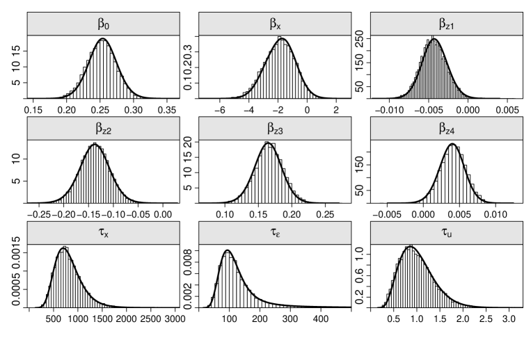
Figure 5: Comparison of the MCMC samples (histograms) with the INLA posterior marginals (lines) for the ibex data. The $\bm{z}$-covariates are those treated as error-free. They are the length of the time series ($\bm{z}_{1}$), average precipitation in summer ($\bm{z}_{2}$), average precipitation in winter ($\bm{z}_{3}$) and the interaction $\bm{z}_{4}=\bm{z}_{1}\bm{z}_{2}$.

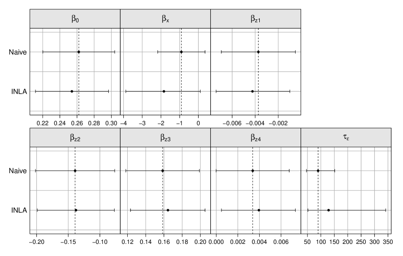
Figure 6: Posterior means and 95% credible intervals in the ibex data analysis. The dashed lines indicate the naive estimates. Only parameters where a naive estimate was available are included here.

5.2 Influence of systolic blood pressure on coronary heart disease

The outcome $y_{i}\in[0,1]$ in this study is an indicator for coronary heart disease, assumed to be Bernoulli distributed. The observation model is logistic, using an indicator for smoking, $\bm{z}$, and the transformed (unobserved) long-term blood pressure $\bm{x}=\log(\text{SBP}-50)$ as binary and continuous covariates, respectively. Hence, the linear predictor is

$$\text{logit}\left[\operatorname{\mathsf{Pr}}(\bm{y}=1\,|\,\bm{x},\bm{z})\right]=\beta_{0}\bm{1}+\beta_{x}\bm{x}+\beta_{z}\bm{z}\ .$$

Since the SBP has been measured at two different examinations, the magnitude of the measurement error of these surrogate measures can be quantified. Here, we assume that the repeated measurements $\bm{w}_{1}$ and $\bm{w}_{2}$ at examination 1 and 2, respectively, are independent and normally distributed with mean $\bm{x}$ and precision $\tau_{u}$, leading to the classical homoscedastic error model

$$\bm{w}\,|\,\bm{x}\sim\mathcal{N}\left(\begin{pmatrix}\bm{x}\\ \bm{x}\end{pmatrix},\tau_{u}\mathbf{I}\right)\ ,$$

where $\bm{w}=(\bm{w}_{1}^{\top},\bm{w}_{2}^{\top})^{\top}$, and $\mathbf{I}$ is of dimension $2n\times 2n$ with $n=641$.

Finally, the exposure model (6) comes in its most general form

$$\bm{x}\,|\,\bm{z}\sim\mathcal{N}(\alpha_{0}\bm{1}+\alpha_{z}\bm{z},\tau_{x}\mathbf{I})\ .$$

The latent field in this model is $\bm{v}=(\bm{x}^{\top},\beta_{0},\beta_{z},\alpha_{0},\alpha_{z})^{\top}$, and the hyperparameters are $\bm{\theta}=(\beta_{x},\tau_{u},\tau_{x})^{\top}$.

For $\beta_{0}$, $\beta_{x}$ and $\beta_{z}$ we assigned independent $\mathcal{N}(0,10^{-2})$ priors. The remaining prior distributions are specified based on prior considerations. We assume that $90$ mmHg and $180$ mmHg can be regarded as the respective $2.5\%$ and $97.5\%$ quantile of SBP, and that $\text{SBP}-50\sim\text{LogNormal}(\mu,\sigma^{2})$. Through optimization we determined $\mu\approx 4.3$ and $\sigma^{2}\approx 0.1$, so that the log normal distribution has the desired quantiles. Consequently, we used $1/\sigma^{2}$ as expected value for $\tau_{x}$. Assuming equal mean and variance for $\tau_{x}$ we specified $\tau_{x}\sim\text{G}(10,1)$, and further $\alpha_{0}\sim\mathcal{N}(0,1)$, whereas $\mu=0$ is used instead of $\mu=4.3$ due to the centering of $\bm{w}_{1}$ and $\bm{w}_{2}$. Rothe and Kim (1980) found the measurement error of SBP to be as much as $20$ mmHg, meaning that our assumed mean SBP of $135$ mmHg varies between $115$ and $155$. This corresponds to an error factor of $1.15$, from which we derive an expected value of approximately $100$ for $\tau_{u}$. Assuming again equal mean and variance of the prior for the precision, we set $\tau_{u}\sim\text{G}(100,1)$. For $\alpha_{z}$ we assume a mean of zero, and set $\alpha_{z}\sim\mathcal{N}(0,1)$. Note, that these prior specifications might deviate from the reference example in Carroll et al. (2006), where the exact parameters were not given. Furthermore, Carroll et al. (2006) used the quantity $\Delta:=\tau_{x}/\tau_{u}$ instead of $\tau_{u}$, and gave it a uniform prior in the interval $(0,0.5)$. Since this is not straightforward with INLA, the model was modified as described.

To obtain Markov Chain Monte Carlo (MCMC) posterior marginals, regression coefficients of GLMs cannot directly be sampled from a standard full conditional distribution. Here, samples were obtained according to Gamerman (1997). The algorithm can be used if the observations $y_{i}$ are conditionally independent and follow an exponential family density. For the regression coefficients $\bm{\beta}=(\beta_{0},\beta_{x},\bm{\beta}^{\top}_{z})^{\top}$, this approach uses transition densities that combine the weighted least squares method with a prior on $\bm{\beta}$ (McCullagh and Nelder, 1989; West, 1985). The full conditionals for the unknowns in our logistic regression model are given in Section 8.1 of the Supplementary Material.

The simulation was run for 100 000 iterations with a burn-in of 10 000, and every 5^th value was saved. Starting values for $\bm{\alpha}$ and $\bm{\beta}$ were chosen from the INLA output. For $\tau_{u}$ and $\tau_{x}$, the mean of their respective prior distribution were used as initial estimates.

The agreement between the MCMC and INLA output is almost perfect, compare supplementary Figure 1. Figure 7 shows parameter estimates for $\beta_{x}$ and $\beta_{z}$ obtained by the naive regression model including $\bm{w}_{1}$ and $\bm{w}_{2}$ instead of $\bm{x}$, and four error-correction approaches. Carroll et al. (2006) used a measurement error model fitted via a maximum-likelihood method and a Bayesian approach using MCMC, denoted here as C.ML and C.MCMC. The fourth and fifth rows show the results obtained by our MCMC implementation and INLA. All error-corrected estimates and the credible intervals are similar. While the coefficient $\beta_{z}$ of the error-free measured smoking status seems unbiased, the effect of systolic blood pressure is clearly attenuated in the naive analysis. Adjusting for measurement error leads to a more pronounced effect, as expected however with a larger assigned uncertainty.

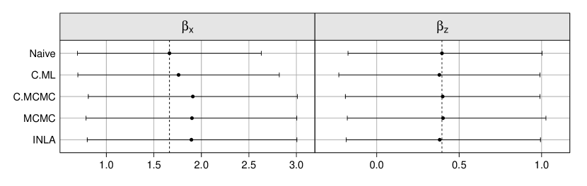
Figure 7: Posterior means and 95% credible intervals for the Framingham data analysis. For MCMC and INLA, posterior means are used as point estimates. C.MCMC and C.ML stand for the Bayesian and the maximum likelihood analysis conducted in Carroll et al. (2006). The dashed lines indicate the naive estimates.

5.3 Seedling growth across different light conditions

Let $\bm{y}$ denote the number of new leaves per plant after a four months growth phase. The covariate $\bm{z}$ denotes the degree of defoliation and $\bm{x}=\log(\%\text{light})$ the (transformed) light intensity, where $\bm{w}$ is the respective target value. Using $\bm{w}$ instead of $\bm{x}$ in the analysis leads to the homoscedastic Berkson error with

$$\bm{x}\,|\,\bm{w}\sim\mathcal{N}(\bm{w},\tau_{u}\mathbf{I})\ .$$

In the following we centered both covariates $\bm{w}$ and $\bm{z}$. This data structure leads to a Poisson regression model with nested design. To account for overdispersion, independent normal random effects $\gamma_{ijk}\sim\mathcal{N}(0,\tau_{\gamma})$ were added, extending the GLM to a GLMM:

$$\log(\operatorname{\mathsf{E}}(y_{ijk}\,|\,\bm{x},\bm{z},\bm{\beta},\bm{\gamma}))=\beta_{0}+\beta_{x}x_{ij}+\beta_{z}z_{k}+\gamma_{ijk}\ ,$$

with $i=1,2,3$ denoting the light condition, $j=1,\ldots,5$ the shadehouse per light condition, and $k=1,\ldots,4$ the degrees of defoliation. The unknowns of this model are $\bm{v}=(\bm{x}^{\top},\beta_{0},\beta_{z})^{\top}$ and $\bm{\theta}=(\beta_{x},\tau_{u},\tau_{\gamma})^{\top}$.

The $\bm{\beta}$ parameters were assigned independent $\mathcal{N}(0,10^{-2})$ priors, and the overdispersion precision $\tau_{\gamma}$ a highly dispersed but proper $\text{G}(1,0.005)$ prior with mean 200. For the error precision $\tau_{u}$ it was assumed that the actual light values $\bm{x}$ do not interfere with the target values $\bm{w}$ from other light levels. The (centered and log-transformed) target light values are 1.22, 0.10 and -1.32 for dark, middle and light conditions, thus the interval between middle and light measurements is 1.42. Interpreting this as one branch of a 95% confidence interval of a Gaussian variable, we obtain $\sigma_{u}=1.42/1.96=0.72$, yielding a lower bound for $\tau_{u}$ of $1/0.72^{2}=1.93$. For the upper bound ten times less variation is assumed, leading to an upper limit of $1/0.072^{2}=193$. The gamma distribution with the respective 2.5% and 97.5% quantiles is $\tau_{u}\sim\text{G}(1,0.02)$.

The results from the regression with INLA were compared to an MCMC run with 100 000 iterations, a burn-in of 10 000 iterations, and a saving frequency of 10. Sampling was based on a reparameterization as proposed by Besag et al. (1995), where all except one full conditional distribution are standard and can be Gibbs-sampled. The MCMC samples and posterior marginals fit very well, see supplementary Figure 2. The parameter estimates from the naive analysis including $\bm{w}$ and the error-corrected estimates of INLA are shown in Figure 8. As mentioned in the introductory Section 2.3, we observe no bias in the regression coefficients, yet there is a small bias in the precision of the random effect $\tau_{\gamma}$. Moreover, the credible intervals for $\beta_{0}$, $\beta_{x}$ and $\tau_{\gamma}$ are slightly increased. Note that the same framework as presented here can be used for logistic regression models, where Berkson error is known to cause bias in the parameter estimates (Burr, 1988; Bateson and Wright, 2010).

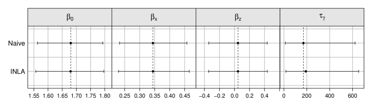
Figure 8: Posterior means and 95% credible intervals for the seedling growth example. The dashed lines indicate the naive estimates. Only parameters where a naive estimate was available are included here.

6 Discussion

Measurement error in covariates may lead to serious biases in parameter estimates and confidence intervals of statistical models. A variety of approaches to model such error have been proposed in the past decades, among which Bayesian methods probably provide the most flexible framework. Bayesian treatments, employing MCMC samplers, have been successfully applied for more than 20 years, but their application has never become part of standard regression analyses.

The aim of this work was to illustrate how the most common ME models (classical and Berkson error) can be included in GLMMs using the recently proposed INLA framework, which gives fast and accurate approximations instead of doing any sampling. The provided R-code should help to make such models accessible to a broader audience. Note that INLA provides a much larger variety of likelihood functions and latent models than we could illustrate here, and the modular structure adds to its flexibility. It is, for instance, straightforward to treat several mismeasured covariates jointly, to introduce a systematic bias into the error model, or to include any structured random term into the model formulation. Gaussian classical and Berkson error models naturally fit into the INLA framework of latent Gaussian models, and thus the error-prone covariates used here are always continuous.

The treatment of more general error models is also possible. One interesting application, relevant for example in ecology, is the use of non-Gaussian error models, for example a Poisson or negative binomial model, where instead of the true and positive (but unobserved) continuous covariate $\bm{x}$, a discrete proxy $\bm{w}$ with mean $\bm{x}$ is observed. More general models might also be useful, e.g. a log-linear model with mean $\operatorname{\mathsf{E}}(\bm{w})=a\bm{x}^{\beta_{x}}$ or a logistic model for binomial proxies. Furthermore, it might not always be appropriate to assume that the components of $\bm{x}$ are iid. Hence, $\bm{x}$ could follow a more complex Gaussian Markov random field structure (Rue and Held, 2005) to account for temporal and/or spatial dependencies, see Bernardinelli et al. (1997) for such a formulation in an epidemiological context. Both of these extensions can be handled with INLA and will be detailed in future work.

One of the biggest challenges when treating mismeasured variables is the estimation of the error variance, either from repeated measurements, instrumental variables or from previous studies. The advantage of a Bayesian approach, as the one taken here, is that uncertainty of such estimates can be incorporated into prior distributions. Sensitivity to chosen prior assumptions can be easily checked due to the computational speed of INLA, see Roos and Held (2011).

Supplementary Material for “Measurement error in GLMMs with INLA”

Due to space constraints, the R-code for all examples presented here is described in detail in the supplementary document. Furthermore, this document contains full conditionals and posterior marginals for Section 5.2. On www.r-inla.org/examples/case-studies/muff-etal-2013 selected data and R-code are provided for download.

Supplementary Material for “Bayesian analysis of measurement error models using INLA"

7 R-code for the three applications in the main text

In this section we guide the reader through the r-inla code and technical details of the three examples discussed in the main text. On www.r-inla.org/examples/case-studies/muff-etal-2013 selected data and R-code are provided for download. The r-inla package can be installed by typing the following command line in the R terminal:

 source("http://www.math.ntnu.no/inla/givemeINLA.R") upgrade.inla(testing=TRUE) Using

 inla.version() information regarding the actual installed version is shown. Here, we used the r-inla version built on July 13, 2013. For more information regarding the installation process we refer to www.r-inla.org.

7.1 Inbreeding in Swiss ibex populations (classical error)

Let all variables be defined as in Section 5.1 of the main text. Recall that the model is Gaussian and contains five covariates ($\bm{x},\bm{z}_{1},\bm{z}_{2},\bm{z}_{3}$ and $\bm{z}_{4}$). The covariate $\bm{x}$ is not directly observed, but only a proxy $\bm{w}$ following a classical heteroscedastic error model $\bm{w}\,|\,\bm{x}\sim\mathcal{N}(\bm{x},\tau_{u}\mathbf{D})$. The prior distributions are elicited from expert/prior knowledge, see main text, and are defined as:

• $\bm{x}\sim\mathcal{N}(\bm{0},\tau_{x}\mathbf{I})$.

• $\beta_{0},\beta_{x},\beta_{z_{1}},\beta_{z_{2}},\beta_{z_{3}},\beta_{z_{4}}\sim\mathcal{N}(0,\tau_{\beta})$, with $\tau_{\beta}=0.0001$,

• $\tau_{x}\sim\text{G}(\alpha_{x},\beta_{x})$, with $\alpha_{x}=1$ and $\beta_{x}=0.0009$,

• $\tau_{y}\sim\text{G}(\alpha_{y},\beta_{y})$, with $\alpha_{x}=1$ and $\beta_{x}=0.001$,

• $\tau_{u}\sim\text{G}(\alpha_{u},\beta_{u})$, with $\alpha_{u}=8.5$ and $\beta_{u}=7.5$.

The object data consists of seven columns:

$$\bm{y}\,\quad\bm{w}\,\quad\bm{z}_{1}\,\quad\bm{z}_{2}\,\quad\bm{z}_{3}\,\quad\bm{z}_{4}\,\quad\text{\bf error.prec}$$

They contain (for $n=26$):

• $y_{1}\ldots y_{n}$: The populations’ intrinsic growth rates.

• $w_{1}\ldots w_{n}$: The estimated inbreeding coefficients (proxies for $x_{1}\ldots x_{n}$; centered).

• $z_{11}\ldots,z_{1n}$: Length of the time series (centered).

• $z_{21}\ldots,z_{2n}$: Average precipitation in summer (centered).

• $z_{31}\ldots,z_{3n}$: Average precipitation in winter (centered).

• $z_{41}\ldots,z_{4n}$: Interaction between $\bm{z}_{1}$ and $\bm{z}_{2}$.

• $\text{error.prec}_{1}\ldots\text{error.prec}_{n}$: The error precisions in the estimates $\bm{w}$.

Start with the prior specification process as described above and in the main text:

 data <- read.table("ibex_data4supp.txt", header=T) attach(data)

 prior.beta <- c(0, 0.0001) prior.prec.x <- c(1, 0.0009) prior.prec.y <- c(1, 0.001) prior.prec.u <- c(8.5, 7.5)

 # initial values (mean or mode of prior) prec.x = 1/0.0009 prec.y = 1/0.001 prec.u = 1 Next, we define the INLA model formula. There are four fixed effects ($\beta_{z_{1}}$, $\beta_{z_{2}}$, $\beta_{z_{3}}$, $\beta_{z_{4}}$) and one random effect $\beta_{x}$ belonging to the error-prone covariate $\bm{x}$, where the new mec model is employed for the latter. Note that the heteroscedasticity in the error in $\bm{w}$ is encoded by assigning the vector of error precisions error.prec to the scale option. In the values option, all values of $\bm{w}$ must be listed. The model contains four hyperparameters:

• beta corresponds to $\beta_{x}$, the slope coefficient of the error-prone covariate $\bm{x}$, with a Gaussian prior.

• prec.u is the error precision $\tau_{u}$ with gamma prior.

• prec.x is the precision $\tau_{x}$ of $\bm{x}\sim\mathcal{N}(\alpha_{0}\bm{1},\tau_{x}\mathbf{I})$ with gamma prior.

• mean.x corresponds to the mean $\alpha_{0}$, which is fixed here at $0$ due to covariate centering.

The prior settings are defined in the different entries of the list hyper. The option fixed specifies whether the corresponding quantity should be estimated or fixed at the initial value. The field param captures the prior parameters of the corresponding prior distribution. Gaussian prior distributions are the default for ${\tt beta}$ and ${\tt mean.x}$, while log-gamma distributions are used for the log-transformed precisions ${\tt prec.u}$ and ${\tt prec.x}$. Note hereby that if a variable $\tau$ is gamma distributed with shape parameter $a$ and rate parameter $b$ leading to the mean $a/b$ and variance $a/b^{2}$, then $\log(\tau)$ is log-gamma distributed with the same parameters $a$ and $b$.

 library(INLA) formula <- y ~ f(w, model = "mec", scale = error.prec, values = w,   hyper = list(    beta = list(      param = prior.beta,      fixed = FALSE      ),    prec.u = list(      param = prior.prec.u,      initial = log(prec.u),      fixed = FALSE      ),    prec.x = list(      param = prior.prec.x,      initial = log(prec.x),      fixed = FALSE      ),    mean.x = list(      initial = 0,      fixed = TRUE      )    )  ) + z1 + z2 + z3 + z4 The call of the inla function includes the specifications for $\tau_{\varepsilon}$, the hyperparameter of the Gaussian regression model. These can be controlled via the control.family option. The prior distributions for the intercept $\beta_{0}$ and the fixed effects of the other covariates $\bm{z}_{1},\ldots,\bm{z}_{4}$ are specified in the control.fixed option.

 r <- inla(formula, data = data.frame(y, w, z1, z2, z3, z4, error.prec),           family = "gaussian",           control.family = list(               hyper = list(                  prec = list(param = prior.prec.y,                           initial = log(prec.y),                           fixed = FALSE                  )               )            ),           control.fixed = list(             mean.intercept = prior.beta[1],             prec.intercept = prior.beta[2],             mean = prior.beta[1],             prec = prior.beta[2]           )      ) r <- inla.hyperpar(r, dz = 0.5, diff.logdens = 20) The last command improves the estimates of the posterior marginals for the hyperparameters of the model. The call is optional, but a slightly better agreement with the MCMC posterior marginals was found in this example. To get a quick overview of the results, use the summary command.

 summary(r)

7.2 Influence of systolic blood pressure on coronary heart disease (classical error)

Let all variables be defined as in Section 5.2 of the main text. The outcome is binary in $[0,1]$, and assumed to be binomial distributed, i.e. $\operatorname{{p}}(y_{i})={N\choose y_{i}}\pi_{i}^{y_{i}}(1-\pi_{i})^{1-y_{i}}$, with $N=1$, $\pi_{i}=\exp(\eta_{i})/(1+\exp(\eta_{i}))$ and and $\eta_{i}=\beta_{0}+\beta_{x}x_{i}+\beta_{z}z_{i}$. We have a classical error structure, where the covariate $\bm{x}=(x_{1},\ldots,x_{n})^{\top}$ is not directly observed, but two replicates, $\bm{w}_{1}=(w_{11},\ldots,w_{1n})^{\top}$ and $\bm{w}_{2}=(w_{21},\ldots,w_{2n})^{\top}$ are used as proxy, where $\bm{w}_{1}\sim\mathcal{N}(\bm{x},\tau_{u}\mathbf{I})$ and $\bm{w}_{2}\sim\mathcal{N}(\bm{x},\tau_{u}\mathbf{I})$. The prior distributions are elicited from expert/prior knowledge, see main text, and are defined as:

• $\bm{x}\sim\mathcal{N}(\alpha_{0}+\alpha_{z}\bm{z},\tau_{x}\mathbf{I})$.

• $\beta_{0},\beta_{x},\beta_{z}\sim\mathcal{N}(0,\tau_{\beta})$, with $\tau_{\beta}=0.01$,

• $\alpha_{0}\sim\mathcal{N}(\mu_{\alpha_{0}},\tau_{\alpha_{0}})$, with $\mu_{\alpha_{0}}=0$ and $\tau_{\alpha_{0}}=1$,

• $\alpha_{z}\sim\mathcal{N}(\mu_{\alpha_{z}},\tau_{\alpha_{z}})$, with $\mu_{\alpha_{z}}=0$ and $\tau_{\alpha_{z}}=1$.

• $\tau_{x}\sim\text{G}(\alpha_{x},\beta_{x})$, with $\alpha_{x}=10$ and $\beta_{x}=1$,

• $\tau_{u}\sim\text{G}(\alpha_{u},\beta_{u})$, with $\alpha_{u}=100$ and $\beta_{u}=1$.

The object data consists of four columns:

$$\bm{y}\,\quad\bm{w_{1}}\,\quad\bm{w_{2}}\,\quad\bm{z}$$

They contain (for $n=641$):

• $y_{1}\ldots y_{n}$: The binary response $y_{i}\in\{0,1\}$.

• $w_{11}\ldots w_{1n}$: $\log(\text{SBP}-50)$ at examination 1 (centered).

• $w_{21}\ldots w_{2n}$: $\log(\text{SBP}-50)$ at examination 2 (centered).

• $z_{1}\ldots z_{n}$: Smoking status $z_{i}\in\{0,1\}$.

As described in the main text, the hierarchical model of this example is formulated in INLA as a joint model by applying the copy feature. The full model can be written as

$$\underbrace{\begin{bmatrix}y_{1}&\tt{NA}&\tt{NA}\\ \vdots&\vdots&\vdots\\ y_{n}&\tt{NA}&\tt{NA}\\ \tt{NA}&0&\tt{NA}\\ \vdots&\vdots&\vdots\\ \tt{NA}&0&\tt{NA}\\ \tt{NA}&\tt{NA}&w_{11}\\ \vdots&\vdots&\vdots\\ \tt{NA}&\tt{NA}&w_{1n}\\ \tt{NA}&\tt{NA}&w_{21}\\ \vdots&\vdots&\vdots\\ \tt{NA}&\tt{NA}&w_{2n}\\ \end{bmatrix}}_{{\tt Y}}=\beta_{0}\underbrace{\begin{bmatrix}1\\ \vdots\\ 1\\ \tt{NA}\\ \vdots\\ \tt{NA}\\ \tt{NA}\\ \vdots\\ \tt{NA}\\ \tt{NA}\\ \vdots\\ \tt{NA}\end{bmatrix}}_{{\tt beta.0}}+\beta_{x}\underbrace{\begin{bmatrix}1\\ \vdots\\ n\\ \tt{NA}\\ \vdots\\ \tt{NA}\\ \tt{NA}\\ \vdots\\ \tt{NA}\\ \tt{NA}\\ \vdots\\ \tt{NA}\end{bmatrix}}_{{\tt beta.x}}+\underbrace{\begin{bmatrix}\tt{NA}\\ \vdots\\ \tt{NA}\\ -1\\ \vdots\\ -n\\ 1\\ \vdots\\ n\\ 1\\ \vdots\\ n\end{bmatrix}}_{{\tt idx.x}}+\beta_{z}\underbrace{\begin{bmatrix}z_{1}\\ \vdots\\ z_{n}\\ \tt{NA}\\ \vdots\\ \tt{NA}\\ \tt{NA}\\ \vdots\\ \tt{NA}\\ \tt{NA}\\ \vdots\\ \tt{NA}\end{bmatrix}}_{{\tt beta.z}}+\alpha_{0}\underbrace{\begin{bmatrix}\tt{NA}\\ \vdots\\ \tt{NA}\\ 1\\ \vdots\\ 1\\ \tt{NA}\\ \vdots\\ \tt{NA}\\ \tt{NA}\\ \vdots\\ \tt{NA}\end{bmatrix}}_{{\tt alpha.0}}+\alpha_{z}\underbrace{\begin{bmatrix}\tt{NA}\\ \vdots\\ \tt{NA}\\ z_{1}\\ \vdots\\ z_{n}\\ \tt{NA}\\ \vdots\\ \tt{NA}\\ \tt{NA}\\ \vdots\\ \tt{NA}\end{bmatrix}}_{{\tt alpha.z}}\ .$$

The reader is guided through the r-inla code for this joint model formulation in the following. The terms below the brackets indicate the names as they will be employed in the code. Start with the prior specification process, as described in the main text:

 data <- read.table("fram_data4supp.txt", header=T) attach(data) n <- nrow(data)  #641

 prior.beta <- c(0, 0.01) prior.alpha0 <- c(0, 1) prior.alphaz <- c(0, 1) prior.prec.x <- c(10, 1) prior.prec.u <- c(100, 1)

 # initial values (mean of prior) prec.u <- 100 prec.x <- 10 Second, the response matrix Y and the data vectors are filled according to the naming of the above joint model equation:

 Y <- matrix(NA, 4*n, 3) Y[1:n, 1] <- y Y[n+(1:n), 2] <- rep(0, n) Y[2*n+(1:n), 3] <- w1 Y[3*n+(1:n), 3] <- w2 beta.0 <- c(rep(1, n), rep(NA, n), rep(NA, n), rep(NA, n)) beta.x <- c(1:n, rep(NA, n), rep(NA, n), rep(NA, n)) idx.x <- c(rep(NA, n), 1:n, 1:n, 1:n) weight.x <- c(rep(1, n), rep(-1, n), rep(1, n), rep(1,n)) beta.z <- c(z, rep(NA, n), rep(NA, n), rep(NA,n)) alpha.0 <- c(rep(NA, n), rep(1, n), rep(NA, n), rep(NA, n)) alpha.z <- c(rep(NA, n), z, rep(NA, n), rep(NA, n)) Ntrials <- c(rep(1, n), rep(NA, n), rep(NA, n), rep(NA, n)) data.joint <- data.frame(Y=Y,      beta.0=beta.0, beta.x=beta.x, beta.z=beta.z,      idx.x=idx.x, weight.x=weight.x,      alpha0=alpha.0, alpha.z=alpha.z,      Ntrials=Ntrials)

The next step contains the definition of the INLA formula. There are four fixed effects ($\beta_{0}$, $\beta_{z}$, $\alpha_{0}$ and $\alpha_{z}$) and two random effects. The latter are needed to encode that the values of $\bm{x}$ in the exposure (7) and error model (8) are assigned the same values as in the regression model (6), where $\beta_{x}\bm{x}$ represents a product of two unknown quantities. The two random effects terms are:

• f(beta.x,...): The copy="idx.x" call guarantees the assignment of identical values to $\bm{x}$ in all components of the joint model. As discussed in the main text, $\beta_{x}$ is treated as a hyperparameter, namely the scaling parameter of the copied process $\bm{x}^{\star}$.

• f(idx.x,...) : idx.x contains the $\bm{x}$ values, encoded as an i.i.d. Gaussian random effect, and weighted with weight.x to ensure correct signs in the joint model. The values option contains the vector of all values assumed by the covariate for which the effect is estimated. It must be a numeric vector, a vector of factors or NULL. The precision prec of the random effect is fixed at $\tau=\exp(-15)$. This is necessary as the uncertainty in $\bm{x}$ is already modelled in the second level (column 2 of $\mathbf{Y}$) of the joint model, which defines the exposure component.

 library(INLA) formula <- Y ~  f(beta.x, copy = "idx.x",      hyper = list(beta = list(param = prior.beta, fixed = FALSE))) +    f(idx.x, weight.x, model = "iid", values = 1:n,      hyper = list(prec = list(initial = -15, fixed = TRUE))) +    beta.0 - 1 + beta.z + alpha.0 + alpha.z Since there is no common intercept in the joint model, it has to be explicitly removed using -1. The call of the inla function is given next. The following options need some explanation:

• family: There are three different likelihoods here, namely the binomial likelihood of the regression model and two Gaussian likelihoods, one for the exposure and one for the error model. They correspond to the different columns in the response matrix Y.

• control.family: Specification of the hyperparameters for the three likelihoods, in the same order as given in family. The binomial likelihood does not contain any hyperparameters, thus the respective list is empty. In the second and third likelihoods the hyperparameters $\tau_{x}$ and $\tau_{u}$ need to be specified, respectively.

• control.fixed: Prior specification for the fixed effects.

 r <- inla(formula, Ntrials = Ntrials, data = data.joint,    family = c("binomial", "gaussian", "gaussian"),    control.family = list(        list(hyper = list()),        list(hyper = list(    prec = list(initial = log(prec.x),    param = prior.prec.x,    fixed = FALSE))),        list(hyper = list(    prec = list(initial=log(prec.u),    param = prior.prec.u,    fixed = FALSE)))),    control.fixed = list(        mean = list(beta.0=prior.beta[1], beta.z=prior.beta[1],    alpha.z=prior.alphaz[1], alpha.0=prior.alpha0[1]),        prec = list(beta.0=prior.beta[2], beta.z=prior.beta[2],    alpha.z=prior.alphaz[2], alpha.0=prior.alpha0[2]))  ) r <-inla.hyperpar(r) The last call (inla.hyperpar) is not required. It is used to improve the estimates of the posterior marginals for the hyperparameters using a finer grid in the numerical integration. In this application, only the marginal of $\tau_{x}$ changes slightly by this correction.

7.3 Seedling growth across different light conditions (Berkson error)

Let all variables be defined as in Section 5.3 of the main text. Recall that the model is Poisson and contains the two covariates $\bm{x}$ and $\bm{z}$, and one independent, normal random effect $\bm{\gamma}$ to account for potential overdispersion. The covariate $\bm{x}$ is not directly observed, but only a proxy $\bm{w}$ following a Berkson error model $\bm{x}\,|\,\bm{w}\sim\mathcal{N}(\bm{w},\tau_{u}\mathbf{I})$. The prior distributions are elicited from expert/prior knowledge, see main text, and are defined as:

• $\beta_{0},\beta_{x},\beta_{z}\sim\mathcal{N}(0,\tau_{\beta})$, with $\tau_{\beta}=0.01$,

• $\tau_{\gamma}\sim\text{G}(\alpha_{\gamma},\beta_{\gamma})$, with $\alpha_{\gamma}=1$ and $\beta_{\gamma}=0.005$,

• $\tau_{u}\sim\text{G}(\alpha_{u},\beta_{u})$, with $\alpha_{u}=1$ and $\beta_{u}=0.02$.

Analysis with the meb model

The object data consists of three columns:

$$\bm{y}\,\quad\bm{w}\,\quad\bm{z}$$

They contain (for $n=60$):

• $y_{1}\ldots y_{n}$: The number of new leaves.

• $w_{1}\ldots w_{n}$: $\log(\%\text{light})$ for the target light intensities under dark, middle and light conditions (i.e., only three different values; centered).

• $z_{1}\ldots z_{n}$: Degree of defoliation (0%, 25%, 50%, 75%; centered).

Let us start again with prior specification process in accordance to the main text:

 data <- read.table("shading_data4supp.txt", header=T) attach(data) n <- 60   # number of seedlings s <- 15   # number of shadehouses w <- w + rep(rnorm(s,0,1e-4),each=n/s) individual <- 1:n # id to incorporate individual random effects

 prior.beta <- c(0,0.01) prior.tau <- c(1,0.005) prior.prec.u <- c(1,0.02)

 # initial values (mean of prior) prec.tau <- 1/0.005 prec.u <- 1/0.02

The fourth line contains a trick to ensure that the light values ${\tt w}$ from the $s=15$ shadehouses are not completely identical, because in the new meb model only the unique values of ${\tt w}$ are used. Thus, if two or more elements of ${\tt w}$ are identical, then they refer to the same element in the covariate $\bm{x}$, which is not desired here. Next, we define the meb model formula. The model contains two hyperparameters:

• beta corresponds to $\beta_{x}$, the slope coefficient of the error-prone covariate $\bm{x}$, with a Gaussian prior.

• prec.u is the error precision $\tau_{u}$ with gamma prior.

The prior settings are defined in the different entries of the list hyper. The option fixed specifies whether the corresponding quantity should be estimated or fixed at the initial value. The field param captures the prior parameters of the corresponding prior distribution. A Gaussian prior distribution is the default for ${\tt beta}$, while a gamma distribution is used for ${\tt prec.u}$ (again defined as log-gamma distribution for the log-precision).
The model contains as additional fixed effect the degree of defoliation z, plus an additional i.i.d. random effects term per individual to account for unspecified heterogeneity, specified in f(individual,...), which extends the GLM to a GLMM:

 library(INLA) formula <- y ~  f(w, model="meb", hyper = list(      beta = list(        param = prior.beta,        fixed = FALSE      ),      prec.u = list(        param = prior.prec.u,        initial = log(prec.u),        fixed = FALSE      )    )) +    z +    f(individual, model = "iid", values = 1:n, hyper = list(prec = list(      initial = log(prec.tau),      param = prior.tau  )       )    )

The call of the inla function includes the specification of the family, which is Poisson here and thus includes no additional hyperparameters. The prior distributions for the intercept $\beta_{0}$ and the slope $\beta_{z}$ are specified in the control.fixed option.

 r <- inla(formula, data = data.frame(y, w, z, individual),           family = "poisson",           control.fixed = list(             mean.intercept = prior.beta[1],             prec.intercept = prior.beta[2],             mean = prior.beta[1],             prec = prior.beta[2]),      ) r <- inla.hyperpar(r) summary(r)

Analysis with the copy feature

As described in the main text, as an alternative to the use of the new meb model, the same results can be obtained by employing the copy feature in INLA. The approach is similar to the one taken in Section 7.2. Recall though that in case of Berkson measurement error, the use of the copy feature does not add to the generality of the model and is presented here only for completeness.

The object data now contains an additional fourth column:

$$\bm{y}\,\quad\bm{w}\,\quad\bm{z}\,\quad{\text{\bf sh}}$$

Column sh contains the values sh₁, $\ldots$, sh_n, where sh_i is the index of the shadehouse of seedling $i$. Note that the $n=60$ seedlings are distributed over $s=15$ shadehouses (1 $\leq$ sh_i $\leq 15$), whereas always five shadehouses belong to the same light condition (dark, middle, light). There are thus 15 different correct light intensities ($\bm{x}$, one value per shadehouse), but only 3 different target light intensities ($\bm{w}$, one value per light condition). As the error model in this example is Berkson, the joint model simplifies to two equations and the response matrix has only two columns. The model can be represented as

$$\underbrace{\begin{bmatrix}y_{1}&\tt{NA}\\ \vdots&\vdots\\ \vdots&\vdots\\ y_{n}&\tt{NA}\\ \tt{NA}&-w_{1}\\ \vdots&\vdots\\ \tt{NA}&-w_{s}\\ \end{bmatrix}}_{{\tt Y}}=\beta_{0}\underbrace{\begin{bmatrix}1\\ \vdots\\ \vdots\\ 1\\ \tt{NA}\\ \vdots\\ \tt{NA}\end{bmatrix}}_{{\tt beta.0}}+\beta_{x}\underbrace{\begin{bmatrix}\text{sh}_{1}\\ \vdots\\ \vdots\\ \text{sh}_{n}\\ \tt{NA}\\ \vdots\\ \tt{NA}\end{bmatrix}}_{{\tt beta.x}}+\underbrace{\begin{bmatrix}\tt{NA}\\ \vdots\\ \vdots\\ \tt{NA}\\ -1\\ \vdots\\ -s\end{bmatrix}}_{{\tt idx.x}}+\beta_{z}\underbrace{\begin{bmatrix}z_{1}\\ \vdots\\ \vdots\\ z_{n}\\ \tt{NA}\\ \vdots\\ \tt{NA}\end{bmatrix}}_{{\tt beta.z}}+\underbrace{\begin{bmatrix}1\\ \vdots\\ \vdots\\ n\\ \tt{NA}\\ \vdots\\ \tt{NA}\end{bmatrix}}_{{\tt gamma}}\ .$$ (10)

Terms below the brackets correspond to the names in the R-code.
Let us start again with prior specification process in accordance to the main text:

 data <- read.table("shading_data4supp.txt", header=T) attach(data) w.red <- aggregate(w, by = list(sh), FUN = mean)[,2] n <- 60 # number of seedlings s <- 15 # number of shadehouses

 prior.beta <- c(0,0.01) prior.tau <- c(1,0.005) prior.prec.u <- c(1,0.02)

 # initial values (mean of prior) prec.tau <- 1/0.005 prec.u <- 1/0.02

The aggregate command in the second line aggregates the vector $\bm{w}$ of length $n=60$ into the $15$ (one per shadehouse) unique light values.
Next, the response matrix Y and the data vectors are filled according to the naming of Equation (10):

 Y <- matrix(NA, n+s, 2) Y[1:n, 1] <- y Y[n+(1:s), 2] <- -w.red beta.0 <- c(rep(1, n), rep(NA, s)) beta.x <- c(sh, rep(NA, s)) idx.x <- c(rep(NA, n), 1:s) weight.x <- c(rep(NA, n), -rep(1, s)) beta.z <- c(z, rep(NA, s)) gamma <- c(1:n, rep(NA, s)) data.joint <- data.frame(Y, beta.0, beta.x, idx.x, weight.x, beta.z, gamma)

The definition of the INLA formula is almost analogous to the one in Section 7.2. The main difference is the additional i.i.d. random effects term per individual $\gamma_{ijk}$, specified in f(gamma,...), which extends the GLM to a GLMM:

 library(INLA) formula <- Y ~  beta.0 - 1 +    f(beta.x, copy = "idx.x",  hyper = list(beta = list(param = prior.beta, fixed = FALSE))) +    f(idx.x, weight.x, model = "iid", values = 1:s,  hyper = list(prec = list(initial = -15, fixed = TRUE))) +    beta.z +    f(gamma, model = "iid", values = 1:n,  hyper = list(prec = list(initial = log(prec.tau), param = prior.tau))) As in Section 7.2 we have to explicitly remove the common intercept using -1. The call of the INLA function is as well in analogy to Section 7.2, but there are only two likelihoods involved here: the Poisson likelihood for the regression model and the Gaussian likelihood for the error model. The former has no additional hyperparameters, while in the latter the error precision $\tau_{u}$ needs specification.

 r <- inla(formula, data = data.joint,  family = c("poisson", "gaussian"),  control.family = list(             list(hyper = list()),             list(hyper = list(      prec = list(              initial=log(prec.u),      param = prior.prec.u,      fixed = FALSE)))),  control.fixed = list(             mean.intercept = prior.beta[1],             prec.intercept = prior.beta[2],             mean = prior.beta[1],             prec = prior.beta[2])       ) r <- inla.hyperpar(r) summary(r)

8 Supplements to Sections 5.2 and 5.3 in the main text

8.1 Full conditionals for the MCMC sampler of Section 5.2

Let all variables be defined as in Section 5.2 of the main text, see also the beginning of Section 7.2 in this Supplementary Material for a compact review.

The full conditionals for the unknowns in the regression model are given as follows:
For $\bm{\beta}=(\beta_{0},\beta_{x},\beta_{z})^{\top}$ we have

$$\bm{\beta}\,|\,rest \propto \pi(\bm{y}\,|\,\bm{x},\bm{z})\cdot\pi(\bm{\beta})$$

$$\propto \exp\left(\sum_{i=1}^{n}y_{i}\eta_{i}-\sum_{i=1}^{n}\log(1+e^{\eta_{i}})-\frac{\tau_{\beta}}{2}\bm{\beta}^{\top}\bm{\beta}\right)\ .$$

The $\bm{\alpha}=(\alpha_{0},\alpha_{z})^{\top}$ coefficients can be sampled from a Gaussian distribution. Let $\mathbf{D}$ be the matrix with rows $D_{i}^{\top}:=(1\;\;{z}_{i}^{\top})$, $\mathbf{R}=\begin{pmatrix}\tau_{\alpha_{0}}&0\\ 0&\tau_{\alpha_{z}}\end{pmatrix}$, and $\bm{\mu}=(\mu_{\alpha_{0}},\mu_{\alpha_{z}})^{\top}$. Then

$${\bm{\alpha}}\,|\,rest \propto \pi({\bm{x}}\,|\,rest)\cdot\pi({\bm{\alpha}})$$

$$\propto \exp\left(-\frac{\tau_{x}}{2}({\bm{x}}-\mathbf{D}{\bm{\alpha}})^{\top}({\bm{x}}-\mathbf{D}{\bm{\alpha}})-\frac{1}{2}\left(\bm{\alpha}-\bm{\mu}\right)^{\top}\mathbf{R}\left(\bm{\alpha}-\bm{\mu}\right)\right)$$

$$\sim \mathcal{N}\left((\tau_{x}\mathbf{D}^{\top}\mathbf{D}+\mathbf{R})^{-1}\left(\tau_{x}\mathbf{D}^{\top}{\bm{x}}+\mathbf{R}\cdot\bm{\mu}\right),\tau_{x}\mathbf{D}^{\top}\mathbf{D}+\mathbf{R}\right),$$

where the second argument in the last expression again denotes the precision matrix. To sample from the distribution of the latent variable $\bm{x}$, full conditionals for $x_{i}$ are needed:

$$x_{i}\,|\,rest \propto \pi(y_{i}\,|\,x_{i},z_{i})\cdot\pi(w_{1i}\,|\,x_{i})\cdot\pi(w_{2i}\,|\,x_{i})\cdot\pi(x_{i}\,|\,z_{i})$$

$$\propto \exp\left(y_{i}\eta_{i}-\log(1+e^{\eta_{i}})-\frac{\tau_{u}}{2}\left((w_{1i}-x_{i})^{2}+(w_{2i}-x_{i})^{2}\right)-\frac{\tau_{x}}{2}(x_{i}-\alpha_{0}-\alpha_{z}z_{i})^{2}\right)\ .$$

Finally, the precisions can be sampled from gamma distributions

$$\tau_{x}\,|\,rest \propto \pi({\bm{x}}\,|\,\bm{z})\cdot\pi(\tau_{x})$$

$$\sim \text{G}\left(a_{x}+\frac{n}{2},b_{x}+\frac{1}{2}({\bm{x}}-\mathbf{D}{\bm{\alpha}})^{\top}({\bm{x}}-\mathbf{D}{\bm{\alpha}})\right)\ ,$$

and

$$\tau_{u}\,|\,rest \propto \pi({\bm{w}}\,|\,\bm{x})\cdot\pi(\tau_{u})$$

$$\sim \text{G}\left(a_{u}+n,b_{u}+\frac{1}{2}(\bm{w}_{1}-\bm{x})^{\top}(\bm{w}_{1}-\bm{x})+\frac{1}{2}(\bm{w}_{2}-\bm{x})^{\top}(\bm{w}_{2}-\bm{x})\right)\ .$$

8.2 MCMC and INLA posterior marginals

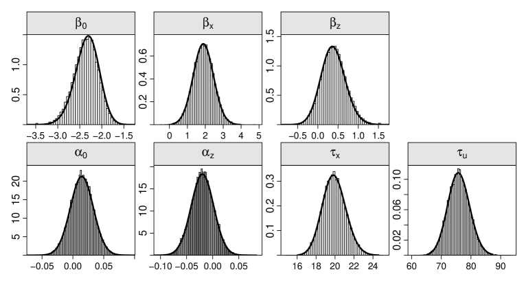
Figure 9: Comparison of the MCMC samples (histograms) with the INLA posterior marginals (lines) for the Framingham data (Section 5.2).

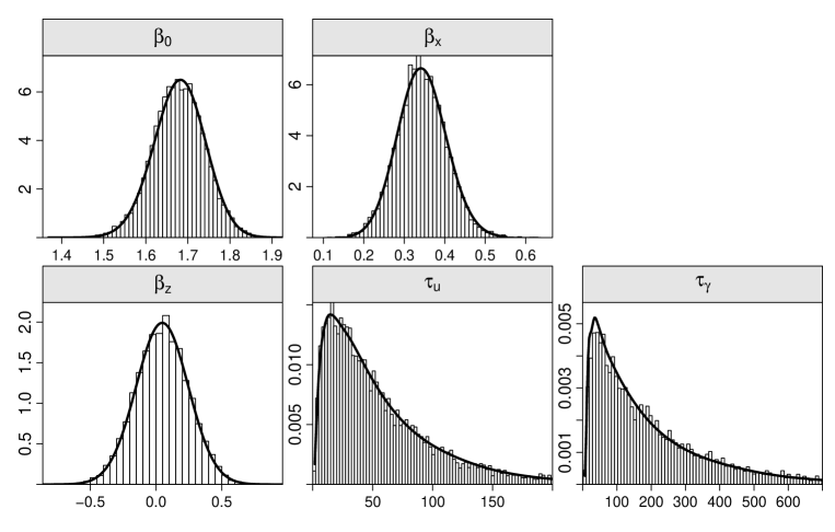
Figure 10: Comparison of the MCMC samples (histograms) with the INLA posterior marginals (lines) for the seedling growth data (Section 5.3).

References

- Bateson and Wright (2010) Bateson, T. F. and J. M. Wright (2010). Regression calibration for classical exposure measurement error in environmental epidemiology studies using multiple local surrogate exposures. American Journal of Epidemiology 172(3), 344–352.
- Berkson (1950) Berkson, J. (1950). Are there two regressions? Journal of the American Statistical Association 45, 164–180.
- Bernardinelli et al. (1997) Bernardinelli, L., C. Pasctto, N. G. Best, and W. R. Gilks (1997). Disease mapping with errors in covariates. Statistics in Medicine 16(7), 741–752.
- Besag et al. (1995) Besag, J., P. Green, D. Higdon, and K. Mengersen (1995). Bayesian computation and stochastic systems (with discussion). Statistical Science 10(1), 3–66.
- Biebach and Keller (2010) Biebach, I. and L. Keller (2010). Inbreeding in reintroduced populations: the effects of early reintroduction history and contemporary processes. Conservation Genetics 11, 527–538.
- Bozzuto et al. (2013) Bozzuto, C., I. Biebach, S. Muff, and L. Keller (2013). Inbreeding effects on population dynamics – the case of Swiss Ibex populations. Technical report, Institute of Evolutionary Biology and Environmental Studies, University of Zurich.
- Buonaccorsi (2010) Buonaccorsi, J. P. (2010). Measurement error. Interdisciplinary Statistics. Boca Raton, FL: CRC Press. Models, methods, and applications.
- Burr (1988) Burr, D. (1988). On errors-in-variables in binary regression—Berkson case. Journal of the American Statistical Association 83(403), 739–743.
- Carroll (1989) Carroll, R. (1989). Covariance analysis in generalized linear measurement error models. Statistics in Medicine 8, 1075–1093.
- Carroll et al. (1985) Carroll, R., P. Gallo, and L. Gleser (1985). Comparison of least squares and errors-in-variables regression, with special reference to randomized analysis of covariance. Journal of the American Statistical Association 80, 929–932.
- Carroll et al. (2006) Carroll, R., D. Ruppert, L. Stefanski, and C. Crainiceanu (2006). Measurement Error in Nonlinear Models: A modern Perspective (2 ed.). Boca Raton: Chapman & Hall.
- Carroll and Stefanski (1990) Carroll, R. and L. Stefanski (1990). Approximate quasilikelihood estimation in models with surrogate predictors. Journal of the American Statistical Association 85, 652–663.
- Carroll et al. (1996) Carroll, R. J., H. Küchenhoff, F. Lombard, and L. A. Stefanski (1996). Asymptotics for the SIMEX estimator in nonlinear measurement error models. Journal of the American Statistical Association 91(433), 242–250.
- Carroll et al. (1984) Carroll, R. J., C. H. Spiegelman, K. K. G. Lan, K. T. Bailey, and R. D. Abbott (1984). On errors-in-variables for binary regression models. Biometrika 71(1), 19–25.
- Clayton (1992) Clayton, D. (1992). Models for the Longitudinal Analysis of Cohort and Case-Control Studies with Inaccurately Measured Exposures. In J. H. Dwyer, M. Feinleib, P. Lippert, and H. Hoffmeister (Eds.), Statistical Models for Longitudinal Studies of Health, pp. 301–331. Oxford University Press.
- Cook and Stefanski (1994) Cook, J. and L. Stefanski (1994). Simulation-extrapolation estimation in parametric measurement error models. Journal of the American Statistical Association 89, 1314–1328.
- Cornfield (1962) Cornfield, J. (1962). Joint dependence of risk of coronary heart disease on serum cholesterol and systolic blood pressure: A discriminant function analysis. Federal Proceedings 21, 58–61.
- Dellaportas and Stephens (1995) Dellaportas, P. and D. Stephens (1995). Analysis of errors-in-variables regression models. Biometrics 51, 1085–1095.
- Fong et al. (2010) Fong, Y., H. Rue, and J. Wakefield (2010). Bayesian inference for generalized linear mixed models. Biostatistics 11(3), 397–412.
- Fuller (1987) Fuller, W. A. (1987). Measurement Error Models. New York: John Wiley & Sons.
- Gamerman (1997) Gamerman, D. (1997). Sampling from the posterior distribution in generalized linear mixed models. Statistics and Computing 7(1), 57–68.
- Gelfand et al. (1996) Gelfand, A., S. K. Sahu, and B. P. Carlin (1996). Efficient parametrizations for generalized linear mixed models. pp. 48–74.
- Gelfand et al. (1995) Gelfand, A. E., S. K. Sahu, and B. P. Carlin (1995). Efficient parametrisations for normal linear mixed models. Biometrika 82(3), 479–488.
- Gelfand and Smith (1990) Gelfand, A. E. and A. F. M. Smith (1990). Sampling-based approaches to calculating marginal densities. Journal of the American Statistical Association 85(410), 398–409.
- Gleser (1990) Gleser, L. (1990). Improvements of the naive approach to estimation in nonlinear errors-in-variables regression models. In P. J. Brown and W. A. Fuller (Eds.), Statistical Analysis of Measurement Error Models and Applications. American Mathematical Society.
- Gleser et al. (1987) Gleser, L., R. Carroll, and P. Gallo (1987). The limiting distribution of least squares in an errors-in-variables regression model. Annals of Statistics 15, 220–233.
- Gustafson (2004) Gustafson, P. (2004). Measurement Error and Misclassification in Statistics and Epidemiology: Impacts and Bayesian Adjustments. Boca Raton: Chapman & Hall/CRC.
- Kannel et al. (1986) Kannel, W., J. Neaton, and D. Wentworth (1986). Overall and coronary heart-disease mortality-rates in relation to major risk-factors in 325’348 men screened for the MRFIT. American Heart Journal 112:4, 825–836.
- Kerber et al. (1993) Kerber, R. A., J. E. Till, S. L. Simon, J. L. Lyon, D. C. Thomas, S. Preston-Martin, M. L. Rallison, R. D. Lloyd, and W. Stevens (1993). A cohort study of thyroid disease in relation to fallout from nuclear weapons testing. Journal of the American Medical Association 270(17), 2076–2082.
- Lunn et al. (2009) Lunn, D., D. Spiegelhalter, A. Thomas, and N. Best (2009). The BUGS project: Evolution, critique, and future directions. Statistics in Medicine 28, 3049–3067.
- Lunn et al. (2000) Lunn, D., A. Thomas, N. Best, and D. Spiegelhalter (2000). WinBUGS – a Bayesian modelling framework: concepts, structure, and extensibility. Statistics and computing 10(4), 325–337.
- MacMahon et al. (1990) MacMahon, S., R. Peto, J. Cutler, R. Collins, P. Sorlie, J. Neaton, R. Abbott, J. Godwin, A. Dyer, and J. Stamler (1990). Blood pressure, stroke and coronary heart disease: Part 1, prolonged differences in blood pressure: Prospective observational studies corrected for the regression dilution bias. Lancet 335, 765–774.
- Martin et al. (2011) Martin, A. D., K. M. Quinn, and J. H. Park (2011). MCMCpack: Markov Chain Monte Carlo in R. Journal of Statistical Software 42(9), 22.
- Martins and Rue (2012) Martins, T. G. and H. Rue (2012, October). Extending INLA to a class of near-Gaussian latent models. ArXiv e-prints. arXiv:1210.1434.
- Martins et al. (2012) Martins, T. G., D. Simpson, F. Lindgren, and H. Rue (2012, October). Bayesian computing with INLA: new features. ArXiv e-prints. arXiv:1210.0333.
- McCullagh and Nelder (1989) McCullagh, P. and J. A. Nelder (1989). Generalized Linear Models (second ed.). Number 37 in Monographs on Statistics and Applied Probability. New York: Chapman and Hall.
- Paine et al. (2012) Paine, T., M. Stenflo, C. Philipson, P. Saner, R. Bagchi, R. Ong, and A. Hector (2012). Differential growth responses in seedlings of ten species of Dipterocarpaceae to experimental shading and defoliation. Journal of Tropical Ecology 28, 377–384.
- Paul et al. (2010) Paul, M., A. Riebler, L. M. Bachmann, H. Rue, and L. Held (2010, Jan). Bayesian bivariate meta-analysis of diagnostic test studies using integrated nested Laplace approximations. Statistics in Medicine 29, 1325–1339.
- Pearson (1902) Pearson, K. (1902). On the mathematical theory of errors of judgement. Philosophical Transactions of the Royal Society of London A 198, 235–299.
- R Core Team (2012) R Core Team (2012). R: A Language and Environment for Statistical Computing. R Foundation for Statistical Computing, Vienna, Austria.
- Richardson and Gilks (1993) Richardson, S. and W. Gilks (1993). Conditional independence models for epidemiological studies with covariate measurement error. Statistics in Medicine 12, 1703–1722.
- Riebler et al. (2012) Riebler, A., L. Held, and H. Rue (2012). Estimation and extrapolation of time trends in registry data - Borrowing strength from related populations. Annals of Applied Statistics 6, 304–333.
- Roos and Held (2011) Roos, M. and L. Held (2011). Sensitivity analysis in Bayesian generalized linear mixed models for binary data. Bayesian Analysis 6(2), 259–278.
- Rothe and Kim (1980) Rothe, C. F. and K. C. Kim (1980, Nov). Measuring systolic arterial blood pressure. Possible errors from extension tubes or disposable transducer domes. Critical Care Medicine 8(11), 683–689.
- Rudemo et al. (1989) Rudemo, M., D. Ruppert, and J. C. Streibig (1989). Random-effect models in nonlinear regression with applications to bioassay. Biometrics 45, 349–362.
- Rue and Held (2005) Rue, H. and L. Held (2005). Gaussian Markov Random Fields: Theory and Applications. London: Chapman & Hall/CRC Press.
- Rue et al. (2009) Rue, H., S. Martino, and N. Chopin (2009, 2). Approximate Bayesian inference for latent Gaussian models by using integrated nested Laplace approximations (with discussion). Journal of the Royal Statistical Society - Series B 71, 319–392.
- Schrödle et al. (2011) Schrödle, B., L. Held, A. Riebler, and J. Danuser (2011). Using INLA for the evaluation of veterinary surveillance data from Switzerland: A case study. Journal of the Royal Statistical Society. Series C (Applied Statistics) 60(2), 261–279.
- Simon et al. (1995) Simon, S. L., J. E. Till, R. D. Lloyd, R. L. Kerber, D. C. Thomas, S. Preston-Martin, J. L. Lyon, and W. Stevens (1995). The Utah leukemia case-control study: dosimetry methodology and results. Health Physics 68(4), 460–471.
- Stephens and Dellaportas (1992) Stephens, D. and P. Dellaportas (1992). Bayesian analysis of generalised linear models with covariate measurement error. In J. M. Bernardo, J. O. Berger, A. P. Dawid, and A. F. M. Smith (Eds.), Bayesian Statistics 4. Oxford Univ Press.
- Subar et al. (2001) Subar, A. F., F. E. Thompson, V. Kipnis, D. Midthune, P. Hurwitz, S. McNutt, A. McIntosh, and S. Rosenfeld (2001). Comparative Validation of the Block, Willett, and National Cancer Institute Food Frequency Questionnaires: The Eating at America’s Table Study. American Journal of Epidemiology 154(12), 1089–1099.
- Wald (1940) Wald, A. (1940). The fitting of straigth lines if both variables are subject to error. Annals of Mathematical Statistics 11, 284–300.
- West (1985) West, M. (1985). Generalized linear models: scale parameters, outlier accommodation and prior distributions. In J. M. Bernardo, M. H. DeGroot, D. V. Lindley, and A. F. M. Smith (Eds.), Bayesian Statistics 2, pp. 531–558. Amsterdam: North-Holland.