Signatures of anisotropic sources in the squeezed-limit bispectrum of the cosmic microwave background

Abstract

The bispectrum of primordial curvature perturbations in the squeezed configuration, in which one wavenumber, $k_{3}$, is much smaller than the other two, $k_{3}\ll k_{1}\approx k_{2}$, plays a special role in constraining the physics of inflation. In this paper we study a new phenomenological signature in the squeezed-limit bispectrum: namely, the amplitude of the squeezed-limit bispectrum depends on an angle between ${\bf k}_{1}$ and ${\bf k}_{3}$ such that $B_{\zeta}(k_{1},k_{2},k_{3})\to 2\sum_{L}c_{L}P_{L}(\hat{\bf k}_{1}\cdot\hat{\bf k}_{3})P_{\zeta}(k_{1})P_{\zeta}(k_{3})$, where $P_{L}$ are the Legendre polynomials. While $c_{0}$ is related to the usual local-form $f_{\rm NL}$ parameter as $c_{0}=6f_{\rm NL}/5$, the higher-multipole coefficients, $c_{1}$, $c_{2}$, etc., have not been constrained by the data. Primordial curvature perturbations sourced by large-scale magnetic fields generate non-vanishing $c_{0}$, $c_{1}$, and $c_{2}$. Inflation models whose action contains a term like $I(\phi)^{2}F^{2}$ generate $c_{2}=c_{0}/2$. A recently proposed “solid inflation” model generates $c_{2}\gg c_{0}$. A cosmic-variance-limited experiment measuring temperature anisotropy of the cosmic microwave background up to $\ell_{\rm max}=2000$ is able to measure these coefficients down to $\delta c_{0}=4.4$, $\delta c_{1}=61$, and $\delta c_{2}=13$ (68% CL). We also find that $c_{0}$ and $c_{1}$, and $c_{0}$ and $c_{2}$, are nearly uncorrelated. Measurements of these coefficients will open up a new window into the physics of inflation such as the existence of vector fields during inflation or non-trivial symmetry structure of inflaton fields. Finally, we show that the original form of the Suyama-Yamaguchi inequality does not apply to the case involving higher-spin fields, but a generalized form does.

UMN-TH-3135/13

1 Introduction

Convincing detection of the so-called “local-form” three-point correlation function (bispectrum) of primordial curvature perturbations from inflation would rule out all single-field inflation models [1, 2], provided that an initial quantum state of the curvature perturbation is in a preferred state called the Bunch-Davies state [3, 4, 5] and that the curvature perturbation does not evolve outside the horizon due to a non-attractor solution [6, 7].

The curvature perturbation, $\zeta$, is defined as a trace part of space-space components of the metric perturbation, $\delta g_{ij}=a^{2}(t)e^{2\zeta}\delta_{ij}$, in a uniform density gauge. The bispectrum of $\zeta$ is defined as $\langle\zeta_{{\bf k}_{1}}\zeta_{{\bf k}_{2}}\zeta_{{\bf k}_{3}}\rangle=(2\pi)^{3}\delta^{(3)}\left({{\bf k}_{1}}+{{\bf k}_{2}}+{{\bf k}_{3}}\right)B_{\zeta}(k_{1},k_{2},k_{3})$, and the local-form bispectrum is defined as $B_{\zeta}(k_{1},k_{2},k_{3})=\frac{6}{5}f_{\rm NL}\left[P_{\zeta}(k_{1})P_{\zeta}(k_{2})+P_{\zeta}(k_{2})P_{\zeta}(k_{3})+P_{\zeta}(k_{3})P_{\zeta}(k_{1})\right]$ (e.g., [8]), where $P_{\zeta}(k)\propto k^{n_{s}-4}$ is the power spectrum of the primordial curvature perturbation with $n_{s}=0.96\pm 0.01$ [9, 10, 11]. This means that the local-form bispectrum has the largest amplitude in the so-called squeezed configuration, in which the smallest wavenumber, $k_{3}$, is much smaller than the other two, i.e., $k_{3}\ll k_{1}\approx k_{2}$ [12]. In this limit the local-form bispectrum is given by $B_{\zeta}\to\frac{12}{5}f_{\rm NL}P_{\zeta}(k_{1})P_{\zeta}(k_{3})$, and all attractor single-field inflation models with a Bunch-Davies initial state give $f_{\rm NL}=\frac{5}{12}(1-n_{s})$ [13, 1].

The current best limit on $f_{\rm NL}$ is $f_{\rm NL}=37\pm 20$ (68% CL), which was obtained from the Wilkinson Microwave Anisotropy Probe (WMAP) 9-year data with the expected ISW-lensing bias removed [14]. The forthcoming Planck data are expected to reduce the error bar by a factor of four [8].

If the Planck collaboration finds evidence for $f_{\rm NL}$, or the lack thereof, what is next? Measuring the local-form four-point function (trispectrum) [15, 16, 17] to check the so-called Suyama-Yamaguchi inequality between the amplitude of the local-form trispectrum and $f_{\rm NL}$, i.e., $\tau_{\rm NL}\geq(6f_{\rm NL}/5)^{2}$ [18, 19, 20, 21, 22, 23, 24, 25], would be an important next step to understand the nature of sources of non-Gaussianity (or the absence thereof). We shall discuss the Suyama-Yamaguchi inequality within the context of higher-spin fields in section 4.

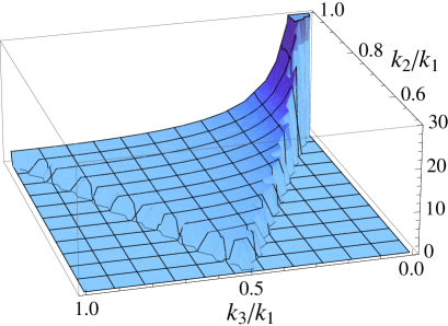
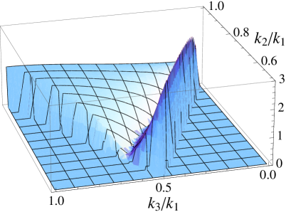
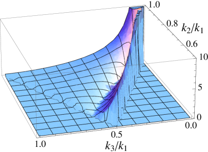
Figure 1: Absolute values of the shape function of $L=0$, $(k_{1}k_{2}k_{3})^{2}S_{0}$ (top left panel), that of $L=1$, $(k_{1}k_{2}k_{3})^{2}S_{1}$ (top right panel), and that of $L=2$, $(k_{1}k_{2}k_{3})^{2}S_{2}$ (bottom panel). We restrict the plot range to $k_{3}\leq k_{2}\leq k_{1}$ and $|k_{1}-k_{2}|\leq k_{3}\leq k_{1}+k_{2}$ for symmetry and the triangular condition. The shape of $L=2$ peaks at the squeezed configuration, $k_{3}/k_{1}\ll 1$ and $k_{2}/k_{1}\approx 1$, in the same way as that of $L=0$ whereas the shape of $L=1$ is suppressed at the squeezed configuration. While the shape function of $L=0$ has positive values for all $k_{2}/k_{1}$ and $k_{3}/k_{1}$, those of $L=1$ and $2$ have negative values except in the flattened configurations, $k_{2}/k_{1}+k_{3}/k_{1}\approx 1$.

Can we learn more about sources of non-Gaussianity by further scrutinizing the behavior of the bispectrum in the squeezed configuration? The answer is yes, and this is the main goal of this paper. Namely, in this paper, we shall investigate phenomenological consequences of the following new parametrization of the bispectrum of primordial curvature perturbations:

$$B_{\zeta}(k_{1},k_{2},k_{3})=\sum_{L}c_{L}P_{L}(\hat{\bf k}_{1}\cdot\hat{\bf k}_{2})P_{\zeta}(k_{1})P_{\zeta}(k_{2})+(\mbox{2 perm})~{},$$ (1.1)

where $P_{L}(\mu)$ is the usual Legendre polynomials, i.e., $P_{0}(\mu)=1$, $P_{1}(\mu)=\mu$, and $P_{2}(\mu)=\frac{1}{2}(3\mu^{2}-1)$. Here, $c_{0}$ is equal to $6f_{\rm NL}/5$.

Why consider $c_{L}$ with $L\geq 1$? These coefficients appear to be sensitive to the existence of vector fields. For example, curvature perturbations sourced by primordial magnetic fields produce non-zero $c_{1}$ and $c_{2}$ [26, 27]. Curvature perturbations sourced by a $\frac{1}{4}I(\phi)^{2}F^{2}$ term in Lagrangian produce $c_{2}=c_{0}/2$ [28, 29]. These coefficients are also sensitive to the existence of a non-trivial realization of SO(3) rotational symmetry during inflation: a recently proposed “solid inflation” model produces $c_{2}\gg c_{0}$ [30]. While the second-order effects in General Relativity also induce non-trivial angular dependence in the bispectrum, it disappears in the squeezed limit [31], and thus will not be considered in this paper.

While we assume that the coefficients, $c_{L}$, do not depend on wavenumbers, it is entirely possible that they do. There are various ways in which $c_{0}=6f_{\rm NL}/5$ depends on wavenumbers [35, 36, 37, 38, 3, 4, 39, 40]. Particularly interesting possibilities are strongly infrared-divergent $c_{1}$ and $c_{2}$, which can naturally give rise to dipoler (i.e., hemispherical) and quadrupolar modulations, respectively, of the observed power spectrum in our sky [41].

In section 2, we shall briefly review these three scenarios to motivate our choice of parametrization given in eq. (1.1). Specifically, we review non-Gaussianities generated from: (1) large-scale magnetic fields after inflation in section 2.1; (2) a vector field coupled to the inflaton field, $\phi$, through a dilaton-like coupling $I^{2}(\phi)F^{2}$ in section 2.2; and (3) solid inflation, in which the inflaton field is a part of a vector multiplet, $\left\{\phi^{1},\phi^{2},\phi^{3}\right\}$, in section 2.3.

What do the shapes of $L=1$ and $L=2$ terms look like? Using the triangular condition of three wavevectors, ${{\bf k}}_{1}+{{\bf k}}_{2}+{{\bf k}}_{3}=0$, the cosine between wavenumbers can be written as, e.g., $\hat{\bf k}_{1}\cdot\hat{\bf k}_{2}=(k_{3}^{2}-k_{1}^{2}-k_{2}^{2})/(2k_{1}k_{2})$. Then, for a scale-invariant power spectrum of $\zeta$, $P_{\zeta}(k)=\frac{2\pi^{2}}{k^{3}}A_{S}$, eq. (1.1) can be re-written as

$$B_{\zeta}(k_{1},k_{2},k_{3})=(2\pi^{2}A_{S})^{2}\sum_{L}c_{L}S_{L}(k_{1},k_{2},k_{3})~{},$$ (1.2)

where

$$S_{0}(k_{1},k_{2},k_{3}) = \left(\frac{1}{k_{1}^{3}k_{2}^{3}}+\mbox{2 perm}\right)~{},$$ (1.3)

$$S_{1}(k_{1},k_{2},k_{3}) = \left(\frac{k_{1}^{2}}{2k_{2}^{4}k_{3}^{4}}+\mbox{2 perm}\right)-\left(\frac{1}{2k_{1}^{4}k_{2}^{2}}+\mbox{5 perm}\right)~{},$$ (1.4)

$$S_{2}(k_{1},k_{2},k_{3}) = \left(\frac{3k_{1}^{4}}{8k_{2}^{5}k_{3}^{5}}+\mbox{2 perm}\right)-\left(\frac{3k_{1}^{2}}{4k_{2}^{5}k_{3}^{3}}+\mbox{5 perm}\right)$$ (1.5)

$$+\left(\frac{3}{8k_{1}^{5}k_{2}}+\mbox{5 perm}\right)+\left(\frac{1}{4k_{1}^{3}k_{2}^{3}}+\mbox{2 perm}\right)~{}.$$

In figure 1, we show the shape functions $S_{0}$ (top left panel), $S_{1}$ (top right one) and $S_{2}$ (bottom one). The bottom panel shows that the bispectrum for $L=2$ peaks in the squeezed limit ($k_{3}\ll k_{1}\approx k_{2}$) in the same way as that for $L=0$, whereas the top right panel shows that the bispectrum for $L=1$ is suppressed in the squeezed limit (also see footnote 2). The bispectrum for $L=1$ peaks when $k_{2}+k_{3}=k_{1}$. This signature may also be seen in the “flattened bispectrum template” defined by eq. (5.1) of ref. [42]. Nevertheless, the correlation coefficient between these bispectra is $0.196$ ; these are only weakly correlated because the flattened template does not change sign while $S_{1}$ is positive in the flattened configurations and is negative otherwise.

The rest of this paper is organized as follows. In section 3, we derive both the full-sky and flat-sky formulae of the bispectrum of temperature anisotropies of the cosmic microwave background (CMB) induced by the angle-dependent bispectrum given in eq. (1.1), and analyze their behaviors. We also estimate the error bars of $c_{L}$ for $L=0$, 1, and 2, expected for a cosmic-variance-limited CMB experiment measuring temperature anisotropy up to $\ell_{\rm max}=2000$. In section 4, we revisit the Suyama-Yamaguchi inequality within the context of higher-spin fields such as those discussed in this paper. We conclude in section 5. In appendix A, we discuss the precision of the flat-sky approximation. In appendix B, we derive the CMB bispectrum in the Sachs–Wolfe limit (in which the temperature anisotropy is given by $\delta T/T=-\zeta/5$). In appendix C, we present the full Fisher matrix for $c_{0}$, $c_{1}$, and $c_{2}$.

Throughout this paper, we adopt the following convention for Fourier transformation of an arbitrary function, $f({\bf x})$: $f({\bf x})=\int\frac{d^{3}{\bf k}}{(2\pi)^{3}}f({\bf k})e^{i{\bf k}\cdot{\bf x}}$.

2 Theoretical motivation

2.1 Helical and non-helical magnetic fields

Astrophysical observations suggest the existence of magnetic fields on the order of $10^{-6}$ G in galaxies and cluster of galaxies [43, 44, 45, 46]. There is also indirect evidence for the existence of magnetic fields on the order of $10^{-20}-10^{-14}$ G in the inter-galactic medium (IGM) [47, 48, 49, 50].

There is yet no compelling model for how these vector fields can be generated during inflation, as the existing models suffer from strong backreaction or strong coupling problems [28, 51, 52, 53, 54, 55] (see the more detailed discussion in the next subsection). Here we simply assume that a magnetic field has been generated, and study its impact on the primordial perturbations during the radiation era and recombination. In the next subsection, we discuss the additional signatures that take place if vector fields are coupled to the inflaton field.

A large amount of literature exist in the studies of effects of vector fields on CMB anisotropies and the large-scale structure of the universe. See, e.g., refs. [58, 59, 60, 61, 62, 63, 64, 65, 66, 67, 68, 69, 70, 71] for effects on the two-point correlation functions, and refs. [72, 73, 74, 75, 76, 77, 78, 26, 27] for those on higher-order correlation functions.

Let us assume that super-horizon vector perturbations were produced during inflation, and they generated large-scale magnetic fields. The anisotropic stress of this magnetic field sources the growth of curvature perturbation via Einstein’s field equations during the radiation era. However, after the decoupling of neutrinos at a few MeV, the magnetic anisotropic stress is compensated by the neutrino anisotropic stress, and the curvature perturbation on super-horizon scales becomes a constant. This constant curvature perturbation survives till the recombination epoch, and seeds additional CMB anisotropies. The solution of curvature perturbations on super-horizon scales is determined by the traceless projection of the magnetic anisotropic stress as [64]

$$\zeta_{\bf k}\approx 0.9\ln\left(\frac{\tau_{\nu}}{\tau_{B}}\right)\left(\hat{k}^{j}\hat{k}_{i}-\frac{1}{3}\delta^{j}_{~{}i}\right)\frac{1}{4\pi\rho_{\gamma,0}}\int\frac{d^{3}{\bf k^{\prime}}}{(2\pi)^{3}}B^{i}({\bf k^{\prime}})B_{j}({\bf k}-{\bf k^{\prime}}),$$ (2.1)

where $\tau_{B}$ and $\tau_{\nu}$ denote the conformal time of the generation of magnetic fields and that of the decoupling of neutrinos, respectively, and $\rho_{\gamma,0}$ is the present-day value of the photon energy density. This equation shows that, even under the assumption that the magnetic field itself is a Gaussian variable, the curvature perturbations become highly non-Gaussian.

Angular dependence of the power spectrum and bispectrum arises due to the spin-1 nature of magnetic fields. The magnetic field vector is transverse, $k^{i}B_{i}=0$, and thus it is expanded using the spin-1 polarization vector, $e_{i}^{(\sigma)}({\hat{\mathbf{k}}})$: $B_{i}({\mathbf{x}})=(2\pi)^{-3}\int d^{3}{\mathbf{k}}~{}B_{i}(\mathbf{k})e^{i{\mathbf{k}}\cdot{\mathbf{x}}}=(2\pi)^{-3}\int d^{3}{\mathbf{k}}~{}\sum_{\sigma=\pm 1}B^{\sigma}(\mathbf{k})e_{i}^{(\sigma)}({\hat{\mathbf{k}}})e^{i{\mathbf{k}}\cdot{\mathbf{x}}}$, where $\sigma$ denotes two circular polarization states. Then, the power spectrum of magnetic fields can be decomposed into the “non-helical,” $P_{B}(k)$, and “helical,” $P_{\cal B}(k)$, components as [79]

$$\left\langle B_{i}({\bf k})B_{j}({\bf k^{\prime}})\right\rangle = -\frac{(2\pi)^{3}}{2}\delta^{(3)}({\bf k}+{\bf k^{\prime}})\sum_{\sigma=\pm 1}\left[P_{B}(k)-\sigma P_{{\cal B}}(k)\right]e_{i}^{(\sigma)}({\hat{\mathbf{k}}})e_{j}^{(-\sigma)}({\hat{\mathbf{k}}})$$ (2.2)

$$= \frac{(2\pi)^{3}}{2}\delta^{(3)}({\bf k}+{\bf k^{\prime}})\left[(\delta_{ij}-\hat{k}_{i}\hat{k}_{j})P_{B}(k)+i\epsilon_{ijl}\hat{k}^{l}P_{{\cal B}}(k)\right],$$

where $\epsilon_{ijl}$ is the antisymmetric tensor normalized as $\epsilon_{123}=1$. These power spectra are defined as

$$-\langle B^{+}({\mathbf{k}})B^{+}({\mathbf{k}}^{\prime})\rangle-\langle B^{-}({\mathbf{k}})B^{-}({\mathbf{k}}^{\prime})\rangle = (2\pi)^{3}P_{B}(k)\delta^{(3)}({\bf k}+{\bf k^{\prime}}),$$ (2.3)

$$\langle B^{+}({\mathbf{k}})B^{+}({\mathbf{k}}^{\prime})\rangle-\langle B^{-}({\mathbf{k}})B^{-}({\mathbf{k}}^{\prime})\rangle = (2\pi)^{3}P_{\cal B}(k)\delta^{(3)}({\bf k}+{\bf k^{\prime}}).$$ (2.4)

Note that the overall sign of the definition of these spectra depends on the choice of the polarization vector.

Using these power spectra, one can write the angle dependence of the bispectrum of curvature perturbations as [27]

$$B_{\zeta}({{\bf k}_{1}},{{\bf k}_{2}},{{\bf k}_{3}}) \propto P_{B}(k_{*})P_{B}(k_{1})P_{B}(k_{2})\left(\frac{1}{3}\mu^{2}_{12}+\mu^{2}_{23}+\mu^{2}_{31}-\frac{2}{3}-\mu_{12}\mu_{23}\mu_{31}\right)$$ (2.5)

$$- P_{B}(k_{*})P_{\cal B}(k_{1})P_{\cal B}(k_{2})\left(\mu_{23}\mu_{31}-\frac{1}{3}\mu_{12}\right)$$

$$+ (1\to 3,~{}2\to 1,~{}3\to 2)+(1\to 2,~{}2\to 3,~{}3\to 1)~{},$$

where $\mu_{ab}\equiv\hat{\bf k}_{a}\cdot\hat{\bf k}_{b}$ and $k_{*}$ denotes some pivot wavenumber.

Eq. (2.5) clearly shows that helical and non-helical magnetic fields generate $L=1$ and $L=2$ angular dependence in the bispectrum of curvature perturbations. If the magnetic field was generated at a GUT scale, i.e., $\tau_{\nu}/\tau_{B}\approx 10^{17}$, with nearly scale-invariant spectra of $P_{B}$ and $P_{\cal B}$, the Legendre coefficients in eq. (1.1) are related to the amplitudes of non-helical and helical magnetic fields smoothed on $1~{}{\rm Mpc}$ as [27]

$$c_{0}\approx-2\times 10^{-4}\left(\frac{B_{1\rm Mpc}}{\rm nG}\right)^{6},\ \ c_{1}\approx-0.9\left(\frac{B_{1\rm Mpc}}{\rm nG}\right)^{2}\left(\frac{{\cal B}_{1\rm Mpc}}{\rm nG}\right)^{4},\ \ c_{2}\approx 14c_{0}.$$ (2.6)

Therefore, if inflation creates $B_{1\rm Mpc}\sim 3{\rm nG}$ and ${\cal B}_{1\rm Mpc}\sim 1{\rm nG}$, which are consistent with the current observational limits, we may have negative and non-vanishing $c_{1}$ and $c_{2}$; namely, $c_{1}\sim-8$ and $c_{2}\sim-2$.

2.2 $I^{2}(\phi)F^{2}$ model

Vector fields with the standard Maxwell $-F^{2}/4$ kinetic term are not produced by the expansion of the universe and, if generated by some other source, they are rapidly diluted away. This poses a challenge to models of primordial magnetogenesis and of vector fields during inflation. Vector fields during inflation can result in broken statistical isotropy of the primordial perturbations, which will be probed by the forthcoming Planck data [81, 82].

Vector fields with a kinetic term given by

$${\cal L}=-\frac{I^{2}\left(\phi\right)}{4}\,F^{2}\;,$$ (2.7)

can instead be produced during inflation if $I\left(t\right)$ has an appropriate time dependence [83]. It is convenient to define the “electric” and “magnetic” components

$$E_{i}=-\frac{I}{a^{2}}A_{i}^{\prime}\;\;,\;\;B_{i}=\frac{I}{a^{2}}\epsilon_{ijk}\partial_{j}A_{k}\;,$$ (2.8)

where the primes denote derivatives with respect to the conformal time, and $a$ is the scale factor of the universe. In terms of these components, the physical energy density in the vector field assumes the conventional expression, $\rho_{A}=\frac{|{\bf E}|^{2}+|{\bf B}|^{2}}{2}$.

If $I\propto a^{n}$, with $n=+2$ or $n=-3$, the magnetic modes are generated during inflation with a scale invariant and frozen spectrum outside the horizon. Rather than assuming that $I$ is an external function, one can obtain the required time dependence by assuming that $I$ is a function of the inflaton $\phi$, with a functional form related to the inflaton potential by [83, 84]

$$I=I_{0}\,{\rm exp}\left[-\int\frac{n\,d\phi}{\sqrt{2\epsilon\left(\phi\right)}M_{p}}\right]\;\;\;\Rightarrow\;\;\;\langle I\rangle\propto a^{n},$$ (2.9)

where $\epsilon$ is the usual slow-roll parameter, $\epsilon\equiv\frac{M_{p}^{2}}{2}\,\left(\frac{1}{V}\frac{dV}{d\phi}\right)^{2}$, with $M_{p}\equiv 1/\sqrt{8\pi G}$ denoting the reduced Planck mass.

Some recent work studied whether this coupling can result in visible cross-correlations between primordial perturbations and large-scale magnetic fields [85, 86, 87, 88, 69, 70, 71]. This is not trivial to realize, as the $n=-3$ choice results in too large an energy density in the electric modes [52, 51], while $n=+2$ leads to too large an electromagnetic coupling constant during inflation [52, 28].

For these reasons, we prefer not to identify the vector field as the electromagnetic field, and we discuss this model only as a mechanism for producing non-Gaussianity. Indeed the vector modes are coupled to the inflaton field by the same $I^{2}\left(\phi\right)F^{2}$ term that generates them, and they source inflaton perturbations through this coupling. These perturbations add up incoherently to the inflaton vacuum modes, and are highly non-Gaussian.

Ref. [89] computed the resulting bispectrum, $\langle\zeta_{{\bf k}_{1}}\zeta_{{\bf k}_{2}}\zeta_{{\bf k}_{3}}\rangle$, in the equilateral configuration, i.e., $k_{1}=k_{2}=k_{3}$. The full bispectrum was computed in refs. [28, 29]. The computations of refs. [28, 29] are restricted to $n=2$ and $n=-2$ which produce, respectively, scale invariant “magnetic” and “electric” perturbations. The model enjoys a symmetry $f\leftrightarrow\frac{1}{f}$, or $n\leftrightarrow-n$, under which $|E|\leftrightarrow|B|$. Both $\pm n$ result in the same equation for $\zeta$. For brevity of exposition, we only refer to the $n=-2$ case in the reminder of this subsection. In this case one obtains, at the leading order in slow-roll,

$$E_{k}\simeq\frac{3H^{2}}{\sqrt{2}k^{3/2}}\;\;,\;\;B_{k}\simeq\frac{H}{\sqrt{2}k^{1/2}a}\;\;,\;\;k\ll aH$$ (2.10)

for the mode functions of each of the two polarizations of the “electric” and the “magnetic” fields in the super-horizon regime [29]. We note that the power in the “electric” field is frozen outside the horizon and scale invariant, whereas the power in the “magnetic” field decreases to negligible values.

Let us assume that, at the beginning of inflation, say at the time $t=0$, the “electric” field has a classical homogeneous value, ${\bf E}^{0}$, all across the universe with negligible perturbations. For $n=-2$, the classical equations of motion for the vector field are solved by a constant, ${\bf E}={\bf E}^{0}$. This quantity is, however, not the classical “electric” field that would be measured by a local observer at $t>0$, which we denote by ${\bf E}_{\rm cl}$. In fact, the modes given by eq. (2.10) become classical after they leave the horizon (we denote them as infra-red (IR) modes), and they add up with ${\bf E}^{0}$ to give ${\bf E}_{\rm cl}$. A given IR mode of wavelength $\lambda$ averages to zero on regions of size $L\gg\lambda$, but it is constant in each region of the size $L\ll\lambda$, and it adds up stochastically with ${\bf E}^{0}$ and with all the other modes with $\lambda\gg L$ generated during inflation to determine the value ${\bf E}_{\rm cl}$ in that region. An observer at time $t>0$ during inflation can only experience the value of ${\bf E}_{\rm cl}$ in its local Hubble patch. The average measured by this observer is drawn from a Gaussian distribution with the mean ${\bf E}^{0}$ and the variance given by

$$\langle{\bf E}\cdot{\bf E}\rangle=\frac{2\times 4\pi}{\left(2\pi\right)^{3}}\int_{Ha\left(t=0\right)}^{Ha\left(t\right)}\frac{dk}{k}k^{3}E_{k}^{2}=\frac{9H^{4}}{2\pi^{2}}\,N,$$ (2.11)

where $N$ is the number of e-folds from the start of inflation to the time $t$. The lower limit in the integral corresponds to the modes that left the horizon at the start of inflation (larger modes are not generated), while the upper limit corresponds to the modes that left the horizon at the time $t$ (larger-momentum modes are still in the quantum regime and do not contribute to the classical average, ${\bf E}_{\rm cl}$, in the Hubble patch of length $\frac{1}{a\left(t\right)H}$).

The situation is completely identical to what happens to the so-called “stochastic inflation [90],” in which the variance of a massless scalar field, $\chi$, is determined by the stochastic addition of the IR modes, and grows as $\langle\chi^{2}\rangle\propto H^{2}N$ during inflation. It is well established in that context that this variance contributes to the theoretical expectation value of the scalar field measure by local observers. This is customary used, for instance, in the Affleck-Dine model of baryogenesis [91] or in the curvaton field [92]. The fact that the vector field has spin $1$ does not make any difference for these considerations, which simply follow from eq. (2.10).

Let us consider a mode, $\zeta_{k}$, of a given comoving momentum, $k$. This mode leaves the horizon $N_{k}$ e-folds before the end of inflation. We are interested in the modes that affect the CMB anisotropies. Such modes leave the horizon $N_{k}\simeq N_{\rm CMB}\simeq 60$ e-folds before the end of inflation. The Hubble patch that they exit is the one that eventually becomes our Hubble patch. When the mode $\zeta_{k}$ leaves the horizon, the classical average of the “electric” field, ${\bf E}_{\rm cl}$, in this Hubble patch is drawn from a Gaussian distribution with the mean ${\bf E}^{0}$ and the variance given by eq. (2.11), with $N=N_{\rm tot}-N_{k}$, where $N_{\rm tot}$ is the total number of e-folds of inflation.

In the presence of this mean, the kinetic term given in eq. (2.7) results in the coupling of ${\cal L}_{\rm int}\simeq 4a^{4}{\bf E}_{\rm cl}\cdot\delta{\bf E}\,\zeta$. This is the dominant operator for the part of $\zeta$ sourced by the vector field [29]. The power spectrum of $\zeta$ generated by this mechanism is given by

$$P_{\zeta}(k)=P_{\zeta}^{(0)}\left(k\right)\left[1+g_{*}\left(k\right)\cos^{2}\theta_{{\hat{k}},{\hat{E}}_{\rm cl}}\right]\;\;,\;\;g_{*}\left(k\right)\simeq-\frac{24E_{\rm cl}^{2}\,N_{k}^{2}}{\epsilon\,V\left(\phi\right)}\;\;,$$ (2.12)

where $P_{\zeta}^{(0)}\equiv\frac{2\pi^{2}}{k^{3}}\frac{H^{2}}{8\pi^{2}\epsilon M_{p}^{2}}$ is the square amplitude of the standard vacuum modes. The second term in eq. (2.12) is the contribution of the sourced part of $\zeta$, which (as phenomenologically required) we have assumed to be subdominant. It follows from the $N_{k}^{2}$ proportionality that this term continues to grow in the super-horizon regime. This power spectrum was previously obtained in refs. [93, 94, 95] in the context of the anisotropic inflationary model [96], where however $E_{\rm cl}$ was identified with ${\bf E}^{0}$, missing the IR contribution.

The $\delta E\,\zeta$ mixing results in the following bispectrum in the squeezed limit, $k_{3}\ll k_{1}\approx k_{2}$ [29]

$$B_{\zeta}(k_{1},k_{2},k_{3}) \simeq 24P_{\zeta}^{(0)}\left(k_{1}\right)P_{\zeta}^{(0)}\left(k_{3}\right)\,|g_{*}\left(k_{1}\right)|N_{k_{3}}$$ (2.13)

$$\times \Bigg{[}1-\cos^{2}\theta_{{\hat{k}}_{1},\,{\hat{E}}_{\rm cl}}-\cos^{2}\theta_{{\hat{k}}_{3},\,{\hat{E}}_{\rm cl}}+\cos\theta_{{\hat{k}}_{1},\,{\hat{E}}_{\rm cl}}\cos\theta_{{\hat{k}}_{3},\,{\hat{E}}_{\rm cl}}\cos\theta_{{\hat{k}}_{1},\,{\hat{k}}_{3}}\Bigg{]}.$$

The predicted power spectrum (eq. 2.12) and bispectrum (eq. 2.13) break statistical isotropy, as ${\bf E}_{\rm cl}$ picks out a preferred direction. However, the prediction for an isotropic measurement is obtained by averaging eq. (2.13) over all directions of ${\hat{E}}_{\rm cl}$. We find

$$B_{\zeta}(k_{1},k_{2},k_{3})\Big{|}_{\rm isotropic\;measurement}\simeq 8P_{\zeta}^{(0)}\left(k_{1}\right)P_{\zeta}^{(0)}\left(k_{3}\right)\,|g_{*}\left(k_{1}\right)|N_{k_{3}}\left(1+\mu_{13}^{2}\right),$$ (2.14)

where $\mu_{13}\equiv\hat{\bf k}_{1}\cdot\hat{\bf k}_{3}$. From this we obtain the Legendre coefficients in eq. (1.1) as

$$c_{0}=32\,\frac{|g_{*}\left(k_{1}\right)|}{0.1}\,\frac{N_{k_{3}}}{60}\;\;\;,\;\;\;c_{2}=\frac{c_{0}}{2}.$$ (2.15)

Due to simplicity of the model, eq. (2.15) is a very predictive result, relating the bispectrum coefficients to the amount of statistical anisotropy of the power spectrum, i.e., $g_{*}$. This result holds for all models characterized by eq. (2.7) and scale invariant “magnetic” or “electric” modes, including many analyses of the magnetogenesis mechanism [83] and of anisotropic inflation [96] (for which the departure from scale invariance is negligibly small; we note that in this work ${\bf E}^{0}$ evolves on an attractor solution, but this has no consequence for the accumulation of the IR modes). An analogous result will also hold for the model of ref. [99] and for the mechanism of ref. [100], for which the scalar perturbations have been studied in ref. [101].

The smallness of $g_{*}$ limits the level of non-Gaussianity. However, a larger bispectrum, for a given value of $g_{*}$, can be obtained if the model is more complicated. For instance, one can arrange for a triplet of U(1) vectors, and assume that they have classical vacuum expectation values which are orthogonal to one another and of equal magnitudes [102]. In this case the power spectrum is statistically isotropic ($g_{*}=0$). This requires to assume that the IR sum is subdominant, as there is no reason to assume that the IR modes of the three vectors add up to orthonormal values. A larger bispectrum can also be obtained if there are additional fields and additional couplings, as in the waterfall mechanism of ref. [103], in which a vector field of the kinetic term given in eq. (2.7) is also coupled to the field that determines the end of hybrid inflation (see ref. [29] for more detailed discussion).

2.3 Solid inflation

Ref. [30] studied a rather unusual model, in which inflation is driven by a system which has a field-theoretical description of a solid. An equivalent version of the model was proposed by ref. [104], under the name of “elastic inflation.”

Each volume element of the solid is characterized by a comoving label, $\phi^{i}$ (for instance, it can be the position of that element at the initial time $t=0$). The functions, $\phi^{i}\left(t,{\bf x}\right)$, specify which volume element is located at a given position, ${\bf x}$, at a given time, $t$. A solid at rest in comoving coordinates then obeys

$$\langle\phi^{1}\rangle=x\;\;,\;\;\langle\phi^{2}\rangle=y\;\;,\;\;\langle\phi^{3}\rangle=z$$ (2.16)

or, in short, $\langle\phi^{i}\rangle=x^{i}$. Even if the vacuum expectation value of each field is ${\bf x}$-dependent, a homogeneous and isotropic Friedmann-Robertson-Walker solution can still be obtained by requiring that the Lagrangian that controls the solid be invariant under rigid translations, $\phi^{i}\rightarrow\phi^{i}+a^{i}$, and SO(3) rotations, $\phi^{i}\rightarrow O^{i}_{j}\phi^{j}$.

At the lowest order in a derivative expansion, the translational invariance is guaranteed by considering functions

$$B^{ij}=g^{\mu\nu}\partial_{\mu}\phi^{i}\partial_{\nu}\phi^{j},$$ (2.17)

and isotropy is obtained by requiring that the Lagrangian is a function of SO(3) invariants built from $B^{ij}$. Only three independent invariants exist, and ref. [30] chose

$$S_{\rm solid}=\int d^{4}x\sqrt{-g}F\left[X,Y,Z\right]\;\;,\;\;X\equiv\left[B\right]\;\;\;,\;\;Y\equiv\frac{\left[B^{2}\right]}{\left[B\right]^{2}}\;\;,\;\;Z\equiv\frac{\left[B^{3}\right]}{\left[B\right]^{3}}\;,$$ (2.18)

where the square parenthesis denotes the trace of the corresponding matrix, e.g., $\left[B\right]\equiv\sum_{i}B^{ii}$.

The system has the energy-momentum tensor, $T^{\mu}_{~{}\mu}={\rm diag}\left(-\rho,p,p,p\right)$, with [30]

$$\rho=-F\;\;,\;\;p=F-\frac{2}{a^{2}}F_{X}\;,$$ (2.19)

where the subscript denotes a partial derivative, and $F$ and $F_{X}$ are evaluated on the background solutions given by $X=\frac{3}{a^{2}\left(t\right)}$, $Y=\frac{1}{3}$, and $Z=\frac{1}{9}$. These invariants are chosen in such a way that $X$ is the only one affected by the overall physical volume expansion; this immediately explains as to why only the derivative of $F$ with respect to $X$ enters into the expression for the pressure.

Inflation is possible only if $F$ is only mildly affected by the physical expansion, or, equivalently, only if $F_{X}$ is sufficiently small. Specifically, we require

$$\epsilon\equiv-\frac{\dot{H}}{H}=\frac{XF_{X}}{F}\ll 1.$$ (2.20)

One also requires $F_{XX}$ to be small, so that $\eta\equiv\frac{\dot{\epsilon}}{\epsilon H}\ll 1$ [30].

Let us now discuss cosmological perturbations in this system. It is convenient to work in a spatially flat gauge, where the dynamical scalar and vector perturbations are all encoded in the perturbations of the scalar fields:

$$\delta\phi^{i}=\pi^{i}\left(t,\,{\bf x}\right)=\frac{\partial_{i}}{\sqrt{-\nabla^{2}}}\,\pi_{L}+\pi_{T}^{i}\;,$$ (2.21)

where the vector components are transverse, $\partial_{i}\pi_{T}^{i}=0$. The scalar and vector modes are decoupled from each other at the linearized level. At the lowest order in the slow roll parameters, and in the deep sub-horizon regime, the sound speeds of the scalar (longitudinal) modes, $c_{L}$, and vector (transverse) modes, $c_{T}$, are given, respectively, by [30]

$$c_{L}^{2}\simeq\frac{1}{3}+\frac{8}{9}\frac{F_{Y}+F_{Z}}{XF_{X}}\;\;,\;\;c_{T}^{2}\simeq\frac{3}{4}\left(1+c_{L}^{2}\right)\;,$$ (2.22)

so that the propagation is subluminal and non-tachyonic ($0<c_{L}^{2}<1$ and $0<c_{T}^{2}<1$) for $0<F_{Y}+F_{Z}<\frac{3}{8}\epsilon|F|$ [30]. Namely, the requirement of an accelerated expansion forces $F_{X}$ to be small, while subluminality also requires that the combination $F_{Y}+F_{Z}$ be small. Finally, the theory involves derivative interactions of the “phonon” fields, $\pi^{i}$, which necessarily become strong at some scale $\Lambda$. A detailed study in ref. [30] gives an estimate of $\Lambda\gg H$ (so that the linearized theory is also valid in the sub-horizon regime, up to $\Lambda$), provided that $\epsilon c_{L}^{3}\gg\left(\frac{H}{M_{p}}\right)^{2/3}$, which can always be obtained for a sufficiently small $H$.

In a conformally flat gauge, the gauge-invariant scalar perturbation, $\zeta$, evaluates to $\zeta=-H\frac{\delta\rho}{\dot{\rho}}=\frac{1}{3}\partial\pi$. Its solution exhibits two features that are peculiar in scalar-field inflation models, but that were nevertheless already seen in the models studied in the previous subsection [28]. The first one is the fact that $\zeta$ is not conserved on super-horizon scales, due to the anisotropic stress that does not vanish on super-horizon scales [30]. Indeed, following ref. [30], we obtain

$$\delta T_{ij,{\rm scalar}}=a^{2}M_{p}^{2}\dot{H}\zeta\left[2\left(3-2\epsilon+\eta\right)\delta_{ij}-\left(3+3c_{L}^{2}-2\epsilon+\eta\right)\left(3{\hat{k}}_{i}\,{\hat{k}}_{j}-\delta_{ij}\right)\right].$$ (2.23)

Let us recall that, also for the model described by eq. (2.7), the anisotropic component of the stress-energy tensor, $\propto E_{{\rm cl},i}\delta E_{j}$, does not vanish outside the horizon, and thus the anisotropic term in eq. (2.12) grows outside the horizon.

The second feature is that, analogously to the model described by eq. (2.7), the bispectrum of solid inflation is largest in the squeezed configurations, and exhibits a nontrivial dependence on the angle between the modes in the squeezed limit. The dominant contribution to the bispectrum is given by the interactions of $\pi$ encoded in the scalar field Lagrangian, while the metric perturbations provide a negligible contribution. The dominant interaction in a slow roll expansion is given by [30]

$${\cal L}\supset M_{p}^{2}a^{3}H^{2}\frac{F_{Y}}{F}\left[\frac{7}{81}\left(\partial\pi\right)^{2}-\frac{1}{9}\partial\pi\partial_{j}\pi^{k}\partial_{k}\pi^{j}-\frac{4}{9}\partial\pi\partial_{j}\pi^{k}\partial_{j}\pi^{k}+\frac{2}{3}\partial_{j}\pi^{i}\partial_{j}\pi^{k}\partial_{k}\pi^{i}\right].$$ (2.24)

Also in this respect, the situation is analogous to the model discussed in the previous subsection, where the dominant contribution to the bispectrum is obtained from eq. (2.7), disregarding metric perturbations. When written in terms of $\zeta$, this interaction exhibits nontrivial dependence on the direction of the modes which does not vanish in the squeezed limit, imprinting the nontrivial angular dependence in the bispectrum.

At the leading order, the Legendre coefficients in eq. (1.1) are given by [30]

$$c_{0}\simeq 0\;\;,\;\;c_{2}={\cal O}\left(1\right)\frac{F_{Y}}{F}\frac{1}{\epsilon c_{L}^{2}}.$$ (2.25)

Namely, in the squeezed limit, the dominant contribution is given by the quadrupole term, whereas the monopole term is negligible. The dominant quadrupole term is essentially proportional to a free combination of parameters (we recall that avoiding superluminality and strong coupling at $p\mathrel{\raise 1.29167pt\hbox{$<$\kern-7.5pt\lower 4.30554pt\hbox{$\sim$}}}H$ imposes restrictions on the combination $F_{Y}+F_{Z}$ but not on $F_{Y}$ or $F_{Z}$ individually).

3 Signatures in the cosmic microwave background

In this section, we shall derive the flat-sky (section 3.1) and full-sky (section 3.2) formulae for the bispectrum of CMB temperature anisotropy from the bispectrum of curvature perturbations given in eq. (1.1). We then calculate, in section 3.3, the error bars of $c_{0}$, $c_{1}$, and $c_{2}$ expected for a cosmic-variance-limited experiment measuring temperature anisotropy up to $\ell=2000$.

3.1 Flat-sky formula

While the full-sky formula is eventually needed for the analysis of full-sky temperature maps, let us derive first the flat-sky formula, as the flat-sky formula is usually simpler and more intuitively understandable.

Under the flat-sky approximation, which is valid only on sufficiently small angular scales, $\ell\gg 1$, CMB fluctuations on the sky are expanded using the two-dimensional Fourier transform, instead of the spherical harmonics. The Fourier coefficients of CMB anisotropy, $a({\boldsymbol{\ell}})$ are related to the three-dimensional coefficients of the curvature perturbation, $\zeta({\bf k})$, as [105]

$$a({\boldsymbol{\ell}}) = \int_{0}^{\tau_{0}}d\tau\int_{-\infty}^{\infty}\frac{dk_{z}}{2\pi}\zeta\left({\bf k}^{\parallel}=-\frac{\boldsymbol{\ell}}{D},k_{z}\right)S_{I}\left(k=\sqrt{k_{z}^{2}+(\ell/D)^{2}},\tau\right)\frac{1}{D^{2}}e^{-ik_{z}D}~{},$$ (3.1)

where ${\bf k}^{\parallel}\equiv(k_{x},k_{y})$, $D\equiv\tau_{0}-\tau$ is the conformal distance out to a given epoch $\tau$, $\tau_{0}$ is the present-day conformal time, and $S_{I}$ is the so-called source function. This relation simply tells us that $a({\boldsymbol{\ell}})$ measures the $\zeta$ modes that are perpendicular to the line-of-sight direction (i.e., the modes on the sky), and the line-of-sight modes are washed out by integration.

It is straightforward to compute the bispectrum of $a({\boldsymbol{\ell}})$ following, e.g., ref. [105]:

$$\left\langle a({\boldsymbol{\ell}_{1}})a({\boldsymbol{\ell}_{2}})a({\boldsymbol{\ell}_{3}})\right\rangle=(2\pi)^{2}\delta^{(2)}\left({\boldsymbol{\ell}}_{1}+{\boldsymbol{\ell}}_{2}+{\boldsymbol{\ell}}_{3}\right)\sum_{L}c_{L}b^{L}(\ell_{1},\ell_{2},\ell_{3})~{},$$ (3.2)

where

$$b^{L}(\ell_{1},\ell_{2},\ell_{3}) \equiv \int_{-\infty}^{\infty}r^{2}dr\left[\prod_{n=1}^{3}\int_{0}^{\tau_{0}}d\tau_{n}\int_{\ell_{n}/D_{n}}^{\infty}\frac{dk_{n}}{2\pi}{\cal G}(\ell_{n},k_{n},\tau_{n},r)\right]$$ (3.3)

$$\times\left[\sum_{n=0}^{L}(\hat{\boldsymbol{\ell}}_{1}\cdot\hat{\boldsymbol{\ell}}_{2})^{n}{\cal F}_{L}^{(n)}\right]P_{\zeta}(k_{1})P_{\zeta}(k_{2})+\mbox{(2 perm)}~{},$$

with

$${\cal G}(\ell,k,\tau,r)\equiv\left[1-\left(\frac{\ell}{kD}\right)^{2}\right]^{-1/2}S_{I}(k,\tau)\frac{2}{D^{2}}\cos\left[\sqrt{1-\left(\frac{\ell}{kD}\right)^{2}}k(r-D)\right]~{}.$$ (3.4)

The other kernel functions, ${\cal F}_{L}^{(n)}$, for $L\leq 2$ are given by ${\cal F}_{0}^{(0)}=1$, ${\cal F}_{1}^{(1)}=\prod_{n=1}^{2}\frac{\ell_{n}}{k_{n}D_{n}}$, ${\cal F}_{2}^{(2)}=\frac{3}{2}\prod_{n=1}^{2}\left(\frac{\ell_{n}}{k_{n}D_{n}}\right)^{2}$, and

$${\cal F}_{1}^{(0)} = -\prod_{n=1}^{2}\sqrt{1-\left(\frac{\ell_{n}}{k_{n}D_{n}}\right)^{2}}\tan\left[\sqrt{1-\left(\frac{\ell_{n}}{k_{n}D_{n}}\right)^{2}}k_{n}(r-D_{n})\right]~{},$$ (3.5)

$${\cal F}_{2}^{(0)} = \frac{3}{2}\prod_{n=1}^{2}\left[1-\left(\frac{\ell_{n}}{k_{n}D_{n}}\right)^{2}\right]-\frac{1}{2}~{},$$ (3.6)

$${\cal F}_{2}^{(1)} = -3\prod_{n=1}^{2}\frac{\ell_{n}}{k_{n}D_{n}}\sqrt{1-\left(\frac{\ell_{n}}{k_{n}D_{n}}\right)^{2}}\tan\left[\sqrt{1-\left(\frac{\ell_{n}}{k_{n}D_{n}}\right)^{2}}k_{n}(r-D_{n})\right]~{}.$$ (3.7)

While these formulae are still complicated, one can read off the leading behaviours of these expressions in the small-scale limit, in which the dominant contributions in the $k$ integration come from the modes with $k\approx\ell/D$. In this limit the kernel functions become ${\cal F}_{1}^{(0)}\to 0$, ${\cal F}_{2}^{(1)}\to 0$, ${\cal F}_{1}^{(1)}\to 1$, ${\cal F}_{2}^{(0)}\to-1/2$, and ${\cal F}_{2}^{(2)}\to 3/2$. We thus find

$$b^{L}(\ell_{1},\ell_{2},\ell_{3}) \to \int_{-\infty}^{\infty}r^{2}dr\left[\prod_{n=1}^{3}\int_{0}^{\tau_{0}}d\tau_{n}\int_{\ell_{n}/D_{n}}^{\infty}\frac{dk_{n}}{2\pi}{\cal G}(\ell_{n},k_{n},\tau_{n},r)\right]$$ (3.8)

$$\times P_{L}(\hat{\boldsymbol{\ell}}_{1}\cdot\hat{\boldsymbol{\ell}}_{2})P_{\zeta}(k_{1})P_{\zeta}(k_{2})+\mbox{(2 perm)}.$$

This result shows that the CMB bispectrum is proportional to $P_{L}(\hat{{\boldsymbol{\ell}}_{1}}\cdot\hat{{\boldsymbol{\ell}}_{2}})$ (and its permutations), which is expected from $P_{L}(\hat{{\bf k}}_{1}\cdot\hat{{\bf k}}_{2})$ (and its permutations) in the three-dimensional bispectrum of the primordial curvature perturbation.

While the approximation of $\ell\approx kD$ gives a simple and transparent result given in eq. (3.8), it is less precise than the original form given by eq. (3.3). In appendix A, we discuss the precision of eqs. (3.3) and (3.8) with respect to the full-sky result given in the next subsection.

3.2 Full-sky formula

Encouraged by the flat-sky results, we now move onto the full-sky case. The CMB temperature anisotropy on the celestial sphere is expanded by the spherical harmonic function as $\delta T(\hat{\bf n})/T=\sum_{\ell,m}a_{\ell m}Y_{\ell m}(\hat{\bf n})$, where $\hat{\bf n}$ is a three-dimensional unit vector pointing toward a given direction on the sky. The spherical harmonics coefficients, $a_{\ell m}$, are related to the primordial curvature perturbation as

$$a_{\ell m} = 4\pi(-i)^{\ell}\int\frac{d^{3}{\bf k}}{(2\pi)^{3}}{\cal T}_{\ell}(k)\zeta_{\mathbf{k}}Y_{\ell m}^{*}(\hat{\mathbf{k}})$$ (3.9)

$$= 4\pi(-i)^{\ell}\int\frac{k^{2}dk}{(2\pi)^{3}}{\cal T}_{\ell}(k)\zeta_{\ell m}(k),$$

where ${\cal T}_{\ell}(k)$ is the so-called radiation transfer function, and we have defined the curvature perturbation expanded in spherical harmonics as $\zeta_{\ell m}(k)\equiv\int d^{2}\hat{\bf k}~{}\zeta_{\bf k}Y_{\ell m}^{*}(\hat{\bf k})$. Then, the bispectrum of $a_{\ell m}$ can be straightforwardly calculated as

$$\left\langle\prod_{n=1}^{3}a_{\ell_{n}m_{n}}\right\rangle=\left[\prod_{n=1}^{3}4\pi(-i)^{\ell_{n}}\int\frac{k^{2}_{n}dk_{n}}{(2\pi)^{3}}{\cal T}_{\ell_{n}}(k_{n})\right]\left\langle\prod_{n=1}^{3}\zeta_{\ell_{n}m_{n}}(k_{n})\right\rangle~{},$$ (3.10)

with the bispectrum of $\zeta_{\ell m}$ related to $B_{\zeta}(k_{1},k_{2},k_{3})$ as

$$\left\langle\prod_{n=1}^{3}\zeta_{\ell_{n}m_{n}}(k_{n})\right\rangle=\left[\prod_{n=1}^{3}\int d^{2}\hat{\bf k}_{n}Y_{\ell_{n}m_{n}}^{*}(\hat{\bf k}_{n})\right](2\pi)^{3}\delta^{(3)}\left({{\bf k}_{1}}+{{\bf k}_{2}}+{{\bf k}_{3}}\right)B_{\zeta}(k_{1},k_{2},k_{3}).$$ (3.11)

Using the bispectrum of $\zeta$ given in eq. (1.1), $B_{\zeta}(k_{1},k_{2},k_{3})$ can be expanded as

$$B_{\zeta}(k_{1},k_{2},k_{3})=P_{\zeta}(k_{1})P_{\zeta}(k_{2})\sum_{L}c_{L}\frac{4\pi}{2L+1}\sum_{M}Y_{LM}^{*}(\hat{{\bf k}}_{1})Y_{LM}(\hat{{\bf k}}_{2})+\mbox{(2 perm)}.$$ (3.12)

Using the definition of the delta function, $\delta^{(3)}({\mathbf{k}})=(2\pi)^{-3}\int d^{3}{\mathbf{x}}~{}e^{i\mathbf{k}\cdot\mathbf{x}}$, we also expand the delta function as

$$\delta^{(3)}\left({{\bf k}_{1}}+{{\bf k}_{2}}+{{\bf k}_{3}}\right) = 8\int_{0}^{\infty}r^{2}dr\left[\prod_{n=1}^{3}\sum_{L_{n}M_{n}}(-1)^{\frac{L_{n}}{2}}j_{L_{n}}(k_{n}r)Y_{L_{n}M_{n}}^{*}(\hat{\bf k}_{n})\right]$$ (3.15)

$$\times\left(\begin{array}[]{ccc}L_{1}&L_{2}&L_{3}\\ M_{1}&M_{2}&M_{3}\end{array}\right)I_{L_{1}L_{2}L_{3}}~{},$$

where the $2\times 3$ matrix denotes the Wigner-3$j$ symbol, and the $I$ symbol is defined by

$$I_{l_{1}l_{2}l_{3}}\equiv\sqrt{\frac{(2l_{1}+1)(2l_{2}+1)(2l_{3}+1)}{4\pi}}\left(\begin{array}[]{ccc}l_{1}&l_{2}&l_{3}\\ 0&0&0\end{array}\right)~{}.$$ (3.18)

Now, performing the integrals of the spherical harmonics over $\hat{{\bf k}}_{1},\hat{{\bf k}}_{2}$, and $\hat{{\bf k}}_{3}$, and performing the summations over $M_{1}$, $M_{2}$, $M_{3}$, and $M$ as described in ref. [106], we obtain

$$\left\langle\prod_{n=1}^{3}\zeta_{\ell_{n}m_{n}}(k_{n})\right\rangle =(2\pi)^{3}B_{\zeta,\ell_{1}\ell_{2}\ell_{3}}(k_{1},k_{2},k_{3})\left(\begin{array}[]{ccc}\ell_{1}&\ell_{2}&\ell_{3}\\ m_{1}&m_{2}&m_{3}\end{array}\right)~{},$$ (3.21)

where

$$B_{\zeta,\ell_{1}\ell_{2}\ell_{3}}(k_{1},k_{2},k_{3}) = 8\int_{0}^{\infty}r^{2}dr\left[\prod_{n=1}^{3}\sum_{L_{n}}(-1)^{\frac{L_{n}}{2}}j_{L_{n}}(k_{n}r)\right]I_{L_{1}L_{2}L_{3}}$$ (3.24)

$$\quad\times\sum_{L}c_{L}\frac{4\pi}{2L+1}I_{\ell_{1}L_{1}L}I_{\ell_{2}L_{2}L}(-1)^{\ell_{2}+L_{1}}\delta_{L_{3},\ell_{3}}$$

$$\quad\times\left\{\begin{array}[]{ccc}\ell_{1}&\ell_{2}&\ell_{3}\\ L_{2}&L_{1}&L\end{array}\right\}P_{\zeta}(k_{1})P_{\zeta}(k_{2})+\mbox{(2 perm)}~{}.$$

Here, the $2\times 3$ matrix enclosed by curly brackets denotes the Wigner-6$j$ symbol. As the primordial bispectrum given by eq. (1.1) is rotationally invariant, the bispectrum expanded in spherical harmonics must also be rotationally invariant. This means that the dependence of the bispectrum on $m_{1},m_{2}$ and $m_{3}$ must be given by the Wigner-$3j$ symbol, as shown in eq. (3.21). This property ensures rotational invariance of the CMB bispectrum.

Substituting eqs. (3.21) and (3.24) into eq. (3.10), we finally obtain the full-sky formula for the CMB bispectrum:

$$\left\langle\prod_{n=1}^{3}a_{\ell_{n}m_{n}}\right\rangle = \left(\begin{array}[]{ccc}\ell_{1}&\ell_{2}&\ell_{3}\\ m_{1}&m_{2}&m_{3}\end{array}\right)B_{\ell_{1}\ell_{2}\ell_{3}}=\left(\begin{array}[]{ccc}\ell_{1}&\ell_{2}&\ell_{3}\\ m_{1}&m_{2}&m_{3}\end{array}\right)\sum_{L}c_{L}B_{\ell_{1}\ell_{2}\ell_{3}}^{L}~{},$$ (3.29)

where

$$B_{\ell_{1}\ell_{2}\ell_{3}}^{L} \equiv \int_{0}^{\infty}r^{2}dr\left[\prod_{n=1}^{3}\sum_{L_{n}}(-1)^{\frac{\ell_{n}+L_{n}}{2}}\right]I_{L_{1}L_{2}L_{3}}\beta_{\ell_{1}L_{1}}(r)\beta_{\ell_{2}L_{2}}(r)\alpha_{\ell_{3}}(r)$$ (3.32)

$$\times\frac{4\pi}{2L+1}I_{\ell_{1}L_{1}L}I_{\ell_{2}L_{2}L}(-1)^{\ell_{2}+L_{1}}\delta_{L_{3},\ell_{3}}\left\{\begin{array}[]{ccc}\ell_{1}&\ell_{2}&\ell_{3}\\ L_{2}&L_{1}&L\end{array}\right\}+\mbox{(2 perm)}~{},$$

and

$$\alpha_{\ell}(r) \equiv \frac{2}{\pi}\int_{0}^{\infty}k^{2}dk~{}{\cal T}_{\ell}(k)j_{\ell}(kr)~{},$$ (3.33)

$$\beta_{\ell L}(r) \equiv \frac{2}{\pi}\int_{0}^{\infty}k^{2}dk~{}P_{\zeta}(k){\cal T}_{\ell}(k)j_{L}(kr)~{}.$$ (3.34)

Owing to the selection rules of the Wigner symbols, $\ell_{1}$, $\ell_{2}$ and $\ell_{3}$ are constrained by parity invariance and the triangular condition:

$$\ell_{1}+\ell_{2}+\ell_{3}={\rm even}~{},\ \ |\ell_{1}-\ell_{2}|\leq\ell_{3}\leq\ell_{1}+\ell_{2}~{}.$$ (3.35)

The former constraint is a consequence of the bispectrum of curvature perturbations given by eq. (1.1) being parity-even. The summation ranges of $L_{1}$ and $L_{2}$ are also restricted to

$$L_{n}=|\ell_{n}-L|,|\ell_{n}-L|+2,\cdots,\ell_{n}+L-2,\ell_{n}+L~{}.$$ (3.36)

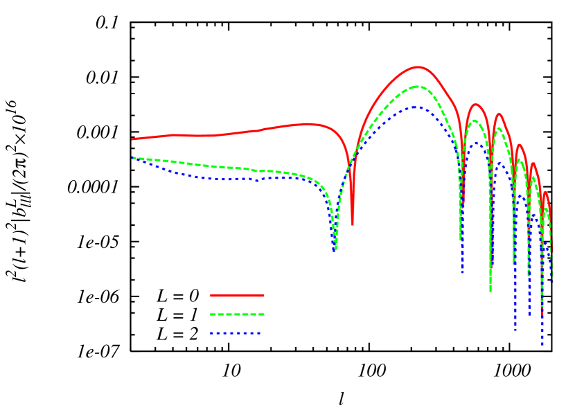
Figure 2: Absolute values of the equilateral CMB temperature reduced bispectra, $|b_{\ell\ell\ell}^{L}|$, for $L=0$ (solid), $L=1$ (long-dashed), and $L=2$ (short-dashed).

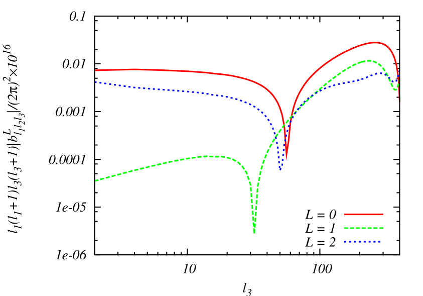
Figure 3: Same as figure 3, but for the squeezed triangles, $|b_{\ell_{1}\ell_{2}\ell_{3}}^{L}|$, with $\ell_{1}=\ell_{2}=200$, as a function of $\ell_{3}$.

In the full-sky formula given by eq. (3.32), the angle dependence for $L>0$ induces a coupling among $\ell_{1}$, $\ell_{2}$ and $\ell_{3}$ via the Wigner-$6j$ symbol. As a result, eq. (3.32) is not separable (or at least not obviously separable) with respect to $\ell$’s unlike the usual local-form CMB bispectrum without angle dependence, i.e., $L=0$.

Figures 2 and 3 show the absolute values of the full-sky reduced bispectra, $b_{\ell_{1}\ell_{2}\ell_{3}}^{L}\equiv B_{\ell_{1}\ell_{2}\ell_{3}}^{L}\left(I_{\ell_{1}\ell_{2}\ell_{3}}\right)^{-1}$, for $L=0$, 1, and 2. Note that the full-sky reduced bispectrum reduces to the flat-sky bispectrum, $b(\ell_{1},\ell_{2},\ell_{3})$, that we discussed in the previous subsection, in the small-sky limit [8].

Figure 2 shows the equilateral triangles with $\ell\equiv\ell_{1}=\ell_{2}=\ell_{3}$, while figure 3 shows triangles with $\ell_{1}=\ell_{2}=200$, which become squeezed triangles for $\ell_{3}\ll 200$. We find that the amplitudes of the equilateral triangles monotonically decrease as $L$ increases. We can understand this by using the flat-sky formula given in eq. (3.8): the Legendre polynomials give the ratio of $L=0$, 1, and 2 terms as

$$b^{L=0}(\ell,\ell,\ell):b^{L=1}(\ell,\ell,\ell):b^{L=2}(\ell,\ell,\ell)=1:-\frac{1}{2}:-\frac{1}{8},$$ (3.37)

for $\hat{\boldsymbol{\ell}}_{i}\cdot\hat{\boldsymbol{\ell}}_{j}=-\frac{1}{2}$ ($i\neq j$).

Figure 3 shows the squeezed triangles with $\ell_{3}\ll\ell_{1}=\ell_{2}=200$. In the squeezed limit, the CMB bispectrum of $L=1$ is highly suppressed compared with those of $L=0$ and 2. This is simply due to symmetry: the $L=1$ term vanishes in the exact squeezed limit. Again, the flat-sky formula given in eq. (3.8) gives the ratio of $L=0$, 1, and 2 terms as

$$b^{L=0}(\ell_{1},\ell_{1},\ell_{3}):b^{L=1}(\ell_{1},\ell_{1},\ell_{3}):b^{L=2}(\ell_{1},\ell_{1},\ell_{3})=1:0:-\frac{1}{2},$$ (3.38)

for $\hat{\boldsymbol{\ell}}_{1}\cdot\hat{\boldsymbol{\ell}_{3}}=0=\hat{\boldsymbol{\ell}}_{2}\cdot\hat{\boldsymbol{\ell}_{3}}$.

As these calculations are quite involved, we provide the simplified analytical formula in the Sachs–Wolfe limit in appendix B. This test validates our numerical results shown in figures 2 and 3.

3.3 Expected uncertainties on $c_{1}$ and $c_{2}$

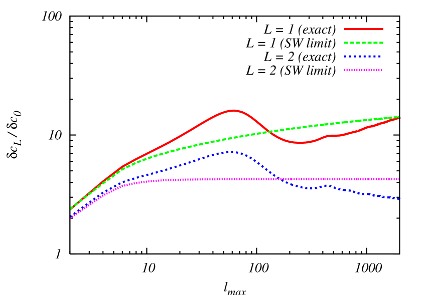
Figure 4: Ratios of the expected error bars, $\delta c_{L}/\delta c_{0}$ ($L=1$ and 2), as a function of the maximum multipoles in the sum, $\ell_{\rm max}$. The solid and short-dashed lines show the exact results for $L=1$ and $L=2$, respectively, while the long-dashed and dotted lines show the corresponding Sachs–Wolfe approximations for $L=1$ and $L=2$, respectively. We find that the Sachs–Wolfe approximations trace the overall behavior of the exact calculations well.

In this subsection, we calculate the 1-$\sigma$ error bars of $c_{0}$, $c_{1}$ and $c_{2}$, i.e., $\delta c_{0}$, $\delta c_{1}$, and $\delta c_{2}$, expected for a cosmic-variance-limited experiment measuring temperature anisotropy. Here, we shall focus on a simultaneous estimation of a pair of parameters: $(c_{0},c_{1})$ and $(c_{0},c_{2})$. We give the full constraint varying all three parameters simultaneously in appendix C.

Following ref. [8], we calculate the Fisher matrix, $F_{LL^{\prime}}$, from

$$F_{LL^{\prime}}\equiv\sum_{2\leq\ell_{1}\leq\ell_{2}\leq\ell_{3}\leq{\ell_{\rm max}}}\frac{B_{\ell_{1}\ell_{2}\ell_{3}}^{L}B_{\ell_{1}\ell_{2}\ell_{3}}^{L^{\prime}}}{\sigma_{\ell_{1}\ell_{2}\ell_{3}}^{2}}~{},$$ (3.39)

where the variance of the CMB bispectrum, $\sigma_{\ell_{1}\ell_{2}\ell_{3}}^{2}$, is given by

$$\sigma_{\ell_{1}\ell_{2}\ell_{3}}^{2}=C_{\ell_{1}}C_{\ell_{2}}C_{\ell_{3}}\left[(-1)^{\ell_{1}+\ell_{2}+\ell_{3}}(1+2\delta_{\ell_{1},\ell_{2}}\delta_{\ell_{2},\ell_{3}})+\delta_{\ell_{1},\ell_{2}}+\delta_{\ell_{2},\ell_{3}}+\delta_{\ell_{3},\ell_{1}}\right]~{},$$ (3.40)

with $C_{\ell}$ being the power spectrum of temperature fluctuations. As we consider a cosmic-variance-limited experiment, we ignore instrumental noise here.

As we show in appendix C, $c_{0}$ and $c_{1}$ are nearly uncorrelated, so are $c_{0}$ and $c_{2}$; however, $c_{1}$ and $c_{2}$ are highly correlated. Therefore, in this subsection, we shall consider submatrices of $F_{LL^{\prime}}$ involving only either $(c_{0},c_{1})$ or $(c_{0},c_{2})$, and study the full matrix in appendix C.

We define the submatrix (a $2\times 2$ matrix) as

$${}^{(2)}F_{ij}\equiv\left(\begin{array}[]{ccc}F_{00}&F_{0L}\\ F_{L0}&F_{LL}\\ \end{array}\right)~{},$$ (3.43)

where $L$ takes on either 1 or 2. The 1-$\sigma$ marginalized error bars are then given by the matrix inverse as $(\delta c_{0},\delta c_{L})=\left(\sqrt{{}^{(2)}F^{-1}_{11}},\sqrt{{}^{(2)}F^{-1}_{22}}\right)$.

In figure 4, we show the ratios of error bars, $\delta c_{1}/\delta c_{0}$ and $\delta c_{2}/\delta c_{0}$, as a function of the maximum multipole in the sum, $\ell_{\rm max}$. The solid and short-dashed lines show the exact results for $L=1$ and $L=2$, respectively, while the long-dashed and dotted lines show the corresponding Sachs–Wolfe approximations for $L=1$ and $L=2$, respectively. We find that the Sachs–Wolfe approximations trace the overall behavior of the exact calculations well.

The error bar on $c_{1}$ is an order of magnitude larger than that on $c_{0}$ for $\ell_{\rm max}\gtrsim 100$, as the $L=1$ bispectrum has a vanishing amplitude in the squeezed limit. On the other hand, the error bar on $c_{2}$ is comparable to that on $c_{0}$: the Sachs–Wolfe approximation gives an asymptotic relation of $\delta c_{2}=4\delta c_{0}$. The exact calculation gives $\delta c_{2}\approx 3\delta c_{0}$ for $\ell_{\rm max}=2000$.

Finally, the 1-$\sigma$ error bars expected for a cosmic-variance-limited experiment measuring temperature anisotropy up to $\ell_{\rm max}=2000$ are given by

$$(\delta c_{0},\delta c_{1}) = (4.4,61)~{},$$ (3.44)

$$(\delta c_{0},\delta c_{2}) = (4.4,13)~{}.$$ (3.45)

See eq. (C.4) for the full Fisher matrix.

4 Consistency relations with higher spin fields

Primordial correlation functions in the limit that some combinations of external momenta go to zero – soft limits – play a special role in constraining the physics of inflation. Significant squeezed non-Gaussianity is associated with the presence of extra light degrees of freedom during inflation, hence soft limits can be understood as probing the spectrum of light fields in the early universe. Moreover, soft limits are observationally relevant and are subject to a number of interesting theoretical consistency relations. The first example of such a consistency relation was noted in ref. [13] and established under much more general conditions in ref. [1]: $\lim_{k_{3}\rightarrow 0}B_{\zeta}(k_{1},k_{2},k_{3})=(1-n_{s})P_{\zeta}(k_{1})P_{\zeta}(k_{3})$. This holds independently of the inflationary Lagrangian, under the assumption that there is only a single field, an attractor solution has been reached [6, 7], and the initial state is in a Bunch-Davies state [3, 4, 5].

Our new parametrization given by eq. (1.1) represents a non-trivial modification of this consistency relation:

$$\lim_{k_{3}\rightarrow 0}B_{\zeta}(k_{1},k_{2},k_{3})=\left(2\sum_{L}c_{L}P_{L}(\hat{\bf k}_{1}\cdot\hat{\bf k}_{3})\right)P_{\zeta}(k_{1})P_{\zeta}(k_{3})\,.$$ (4.1)

The possibility that some of the $c_{L}$ coefficients can be $\gg|n_{s}-1|\sim 10^{-2}$ indicates extra light fields in the early universe, while the non-trivial angular dependence is associated with anisotropic sources (such as higher spin fields). We also expect non-trivial soft limits for higher-order correlation functions. To explore such effects, we introduce the quantities

$$f_{NL}^{\mathrm{eff}}(k_{i}) \equiv \lim_{k_{3}\rightarrow 0}\frac{5}{12}\frac{B_{\zeta}(k_{1},k_{2},k_{3})}{P_{\zeta}(k_{1})P_{\zeta}(k_{3})}\,,$$ (4.2)

$$\tau_{NL}^{\mathrm{eff}}(k_{i}) \equiv \lim_{{\bf k_{1}}+{\bf k_{2}}\rightarrow 0}\frac{1}{4}\frac{T_{\zeta}(k_{1},k_{2},k_{3},k_{4})}{P_{\zeta}(|{\bf k}_{1}+{\bf k}_{2}|)P_{\zeta}(k_{1})P_{\zeta}(k_{3})}\,,$$ (4.3)

where $\langle\zeta_{{\bf k}_{1}}\zeta_{{\bf k}_{2}}\zeta_{{\bf k}_{3}}\zeta_{{\bf k}_{4}}\rangle=(2\pi)^{3}\delta^{(3)}(\sum_{i}{\mathbf{k}}_{i})T_{\zeta}(k_{1},k_{2},k_{3},k_{4})$. For the local-type non-Gaussianity the quantities $f_{NL}^{\mathrm{eff}}$ and $\tau_{NL}^{\mathrm{eff}}$ become the standard (momentum independent) non-linearity parameters. In this case there is an interesting consistency relation:

$$\tau_{NL}\geq\left(\frac{6}{5}f_{NL}\right)^{2}\,,$$ (4.4)

where we dropped the superscript “eff” to emphasize that this relation is understood in the case where eqs. (4.2) and (4.3) are independent of momenta. This relation was first noted by Suyama and Yamaguchi in ref. [18] and further explored in refs. [19, 20, 21, 22, 23, 24, 25].

In this subsection, we explore the non-Gaussianity consistency relations in the context of the $I^{2}(\phi)F^{2}$ model given in eq. (2.7). In general this model breaks statistical isotropy, as discussed in section 2.2. From eq. (2.13) we obtain

$$f_{NL}^{\rm eff}\simeq 10N_{k_{1}}^{2}N_{k_{3}}\frac{24E_{\rm cl}^{2}}{\epsilon V(\phi)}\left[1-\cos^{2}\theta_{{\hat{k}}_{1},\,{\hat{E}}_{\rm cl}}-\cos^{2}\theta_{{\hat{k}}_{3},\,{\hat{E}}_{\rm cl}}+\cos\theta_{{\hat{k}}_{1},\,{\hat{E}}_{\rm cl}}\cos\theta_{{\hat{k}}_{3},\,{\hat{E}}_{\rm cl}}\cos\theta_{{\hat{k}}_{1},\,{\hat{k}}_{3}}\right]\,,$$ (4.5)

where we recall that $|g_{*}(N_{k_{i}})|=N_{k_{i}}^{2}\frac{24E_{\rm cl}^{2}}{\epsilon V\left(\phi\right)}\ll 1$ is assumed.

We compute the trispectrum for the first time in the model given by eq. (2.7). The computation follows very closely the analogous one of the bispectrum performed in ref. [29], and so we omit the technical details. We obtain

$$\!\!\!\!\!\!\!\!\tau_{\rm NL}^{\rm eff}\simeq 144N_{k_{1}}^{2}N_{k_{3}}^{2}\frac{24E_{\rm cl}^{2}}{\epsilon V(\phi)}\Bigg{[} \!\!\!\!1-\cos^{2}\theta_{{\hat{k}}_{1},\,{\hat{E}}_{\rm cl}}-\cos^{2}\theta_{{\hat{k}}_{12},\,{\hat{E}}_{\rm cl}}-\cos^{2}\theta_{{\hat{k}}_{3},\,{\hat{E}}_{\rm cl}}$$ (4.6)

$$+\cos\theta_{{\hat{k}}_{1},\,{\hat{E}}_{\rm cl}}\cos\theta_{{\hat{k}}_{3},\,{\hat{E}}_{\rm cl}}\cos\theta_{{\hat{k}}_{1},\,{\hat{k}}_{3}}$$

$$+\cos\theta_{{\hat{k}}_{1},\,{\hat{E}}_{\rm cl}}\cos\theta_{{\hat{k}}_{12},\,{\hat{E}}_{\rm cl}}\cos\theta_{{\hat{k}}_{1},\,{\hat{k}}_{12}}$$

$$+\cos\theta_{{\hat{k}}_{12},\,{\hat{E}}_{\rm cl}}\cos\theta_{{\hat{k}}_{3},\,{\hat{E}}_{\rm cl}}\cos\theta_{{\hat{k}}_{12},\,{\hat{k}}_{3}}$$

$$-\cos\theta_{{\hat{k}}_{1},\,{\hat{E}}_{\rm cl}}\cos\theta_{{\hat{k}}_{3},\,{\hat{E}}_{\rm cl}}\cos\theta_{{\hat{k}}_{1},\,{\hat{k}}_{12}}\cos\theta_{{\hat{k}}_{12},\,{\hat{k}}_{3}}\Bigg{]},$$

where ${\hat{k}}_{12}$ is the unit vector in the direction of ${\bf k}_{1}+{\bf k}_{2}$. We note that the unit-vector ${\hat{k}}_{12}$ enters in this expression, even though the corresponding vector $\vec{k}_{1}+\vec{k}_{2}$ vanishes in the squeezed limit (analogously to the ${\hat{k}}_{3}$-dependence of the bispectrum).

We observe that, in the $I^{2}(\phi)F^{2}$ model, both $f_{NL}^{\mathrm{eff}}$ and $\tau_{NL}^{\mathrm{eff}}$ exhibit highly non-trivial momentum dependence; thus, it is not sensible to compare different configurations. One can readily see that $\tau_{\rm NL}^{\mathrm{eff}}$ vanishes for several configurations. This happens, for example, if one of ${\hat{k}}_{1}\,,{\hat{k}}_{12}\,,{\hat{k}}_{3}$ is parallel to ${\hat{E}}_{\rm cl}$, while the other two vectors are perpendicular to ${\hat{E}}_{\rm cl}$. We do not interpret this as a violation of the Suyama-Yamaguchi inequality; the expression given by eq. (4.4) requires either that the non-linearity parameters are momentum-independent, or else that $\tau_{NL}^{\mathrm{eff}}$ and $\left(f_{NL}^{\mathrm{eff}}\right)^{2}$ have the same momentum dependence so that one can factor out an amplitude which obeys eq. (4.4). The original form of the Suyama-Yamaguchi inequality is simply not applicable to the model given by eq. (2.7).

In ref. [25] Assassi et al derived a general inequality relating the soft limits of the bispectrum and trispectrum:

$$\int d^{3}q_{1}d^{3}q_{2}\,\,\tau^{\mathrm{eff}}_{NL}({\bf q}_{1},{\bf k}-{\bf q}_{1},{\bf q}_{2},-{\bf q}_{2}-{\bf k})\,\,P_{\zeta}(q_{1})P_{\zeta}(q_{2})$$

$$\geq\left[\int d^{3}q\,\,\frac{6}{5}\,f_{NL}^{\mathrm{eff}}({\bf q},-{\bf q}-{\bf k},{\bf k})\,\,P_{\zeta}(q)\right]^{2}\,,$$ (4.7)

where the $k\rightarrow 0$ limit is understood. This inequality reduces to eq. (4.4) in the local case, but is completely general and should be respected by any model. We can easily verify that, although the Suyama-Yamaguchi inequality is not meaningful here, eq. (4.7) is still respected. After evaluating the angular integral, the left hand side of eq. (4.7) becomes

$${\rm LHS}\simeq 1024\pi^{2}\frac{24E_{\rm cl}^{2}}{\epsilon V(\phi)}\sin^{2}\theta_{{\hat{k}},\,{\hat{E}}_{\rm cl}}\left(\int dq\,q^{2}N_{q}P_{\zeta}\left(q\right)\right)^{2},$$ (4.8)

and, proceeding analogously, the right hand side becomes

$${\rm RHS}\simeq 1024\pi^{2}N_{k}^{2}\left[\frac{24E_{\rm cl}^{2}}{\epsilon V(\phi)}\right]^{2}\sin^{4}\theta_{{\hat{k}},\,{\hat{E}}_{\rm cl}}\left(\int dq\,q^{2}N_{q}P_{\zeta}\left(q\right)\right)^{2}.$$ (4.9)

Therefore, we find

$$\frac{\rm LHS}{\rm RHS}\simeq\frac{1}{|g_{*}\left(N_{k}\right)|\sin^{2}\theta_{{\hat{k}},\,{\hat{E}}_{\rm cl}}}>1.$$ (4.10)

Note that $|g_{*}|\ll 1$ has been assumed (as also required by phenomenology) throughout this subsection. We therefore conclude that the integrated inequality given by eq. (4.7) is satisfied for any orientations of $\vec{k}$ relative to the classical vector field background.

5 Conclusion

The angle dependence of the bispectrum of primordial curvature perturbations in the squeezed configuration is sensitive to the presence of vector fields and non-trivial symmetry during inflation. In this paper, we have explored phenomenological consequences of the new parametrization of the bispectrum given by eq. (1.1): $B_{\zeta}=\sum_{L}c_{L}P_{L}(\hat{\bf k}_{1}\cdot\hat{\bf k}_{2})P_{\zeta}(k_{1})P_{\zeta}(k_{2})+(\mbox{2 perm})$. This form is physically well motivated, and we have given three examples in section 2: the curvature perturbation sourced by the anisotropic stress of magnetic fields; that sourced by an interaction with a vector field of the form $I^{2}(\phi)F^{2}$; and solid inflation.

We find that a cosmic-variance-limited CMB experiment measuring temperature anisotropy up to $\ell_{\rm max}=2000$, such as the Planck satellite, can measure $c_{1}$ and $c_{2}$ down to $\delta c_{1}=61$ and $\delta c_{2}=13$ (68% CL). The latter error bar is comparable to (and only a factor of three larger than) the error bar of $c_{0}=6f_{\rm NL}/5$; thus, if the forthcoming Planck data reveal evidence for $c_{0}$, one should also measure $c_{2}$ to understand the nature of sources of non-Gaussianity. Moreover, even if the Planck data do not reveal evidence for $c_{0}$, one should still measure $c_{2}$, as solid inflation can generate large $c_{2}$ without generating detectable $c_{0}$. Sensitivity to $c_{1}$ is an order of magnitude worse than that to $c_{0}$ or $c_{2}$ because the term proportional to $c_{1}$ vanishes in the squeezed limit due to symmetry.

The angle-dependent bispectrum in the squeezed configuration is a natural consequence of broken statistical isotropy. Broken isotropy also leads to a non-trivial modification of the inequality between the local-form trispectrum amplitude, $\tau_{\rm NL}$, and $f_{\rm NL}^{2}$. We find that the original form of the Suyama-Yamaguchi inequality, $\tau_{\rm NL}\geq(6f_{\rm NL}/5)^{2}$, does not apply to the current model, due to the momentum- and shape-dependence of $\tau_{\rm NL}$ and $f_{\rm NL}$. For example, we find some squeezed configurations in which $\tau_{\rm NL}$ vanishes. It remains to be seen how sensitive the forthcoming tests of the Suyama-Yamaguchi inequality using the Planck or the large-scale structure data are to the decrease of the trispectrum amplitudes for these particular shapes. We also find that a general inequality of ref. [25] is satisfied in this model.

What is next? Phenomenological consequences of eq. (1.1) for large-scale structure of the universe such as the dark matter halo bias [108], bispectrum, and trispectrum should certainly be explored. For instance, a consistency relation [109, 110] between the squeezed bispectrum and the power spectrum of dark matter density fluctuations has been proved at the full nonlinear level, and with an initial isotropic non-Gaussianity, in ref. [109]. It may be interesting to study a signature of anisotropic initial non-Gaussianity in that context. Also, it is quite possible that the coefficients $c_{L}$ depend on wavenumbers, which would be particularly interesting for dipolar and quadrupolar modulations of the observed power spectrum in our sky [41]. Indeed, in the case of the $I^{2}(\phi)F^{2}$ model discussed in section 2.2, the $c_{L}$ coefficients exhibit a logarithmic running with wavenumber. It would be interesting to study possible effects of such wavenumber dependence.

Note added

After our paper was submitted, the Planck collaboration reported constraints on non-Gaussianity parameters [111]. They also evaluated the coefficients $c_{1}$ and $c_{2}$ as follows: they first constrain coefficients of the basis functions of the “modal expansion,” from which they construct templates for the shapes corresponding to $L=1$ and 2 of eq. (1.1). This results in a value of $11.0\pm 113$ (68% CL) for the coefficient $c_{1}$, and of $3.8\pm 27.8$ (68% CL) for the coefficient $c_{2}$. As also remarked in ref. [111], the template used in their analysis is only $60\%$ correlated with $L=2$, suggesting that the estimators constructed from the modal expansion can provide an estimate for these shapes, but that they might not be optimal. Our reported forecast for the 1-$\sigma$ uncertainties, $\delta c_{L}$, assumes a full sky, cosmic-variance-limited experiment measuring temperature anisotropy up to $\ell=2000$. However, the Planck data are noise dominated for $\ell\gtrsim 1500$ and the analysis presented in ref. [111] uses 73% of the sky. Rescaling our estimates by $1/\sqrt{0.73}$ but still assuming a cosmic-variance-limited experiment, we find $\delta c_{0}=5.1$, $\delta c_{1}=71$, and $\delta c_{2}=15$. On the other hand, the Planck collaboration finds $\delta c_{0}=7.0$, $\delta c_{1}=113$, and $\delta c_{2}=28$ (recall that $c_{0}$ is equal to $6f_{\rm NL}/5$). As the Planck collaboration uses the optimal estimator to find a limit on $\delta c_{0}$, we estimate the effect of noise in the Planck data by rescaling the error bars by the ratio of $7.0/5.1$. We find $\delta c_{1}=97$ and $\delta c_{2}=21$. These estimates for $\delta c_{1}$ and $\delta c_{2}$ are $16\%$ and $33\%$ lower than the error bars that the Planck collaboration finds. The latter can be understood from the fact that the template for $L=2$ used by the Planck collaboration is $60\%$ correlated with the true shape. Therefore, it appears that there is still some room for improvement in the limits on these parameters, especially $c_{2}$, using optimal estimators.

Appendix A Precision of the flat-sky approximation

How precise are the flat-sky formulae given by eqs. (3.3) and (3.8)? In figure 5, we compare the full-sky results with the flat-sky results. We find that, for $L=0$ and 1, the simplified flat-sky formula given by eq. (3.8) yields the bispectra in the equilateral and squeezed configurations which are in good agreement with the full-sky results at $\ell\gtrsim 100$. However, we find that, for $L=2$, the simplified formula systematically underestimate the magnitude of the bispectra in both configurations. The equilateral result suggests that the simplified formula provides an adequate result only at $\ell\gtrsim 800$.

While these results appear to suggest that the precision of the simplified formula degrades as $L$ increases, this is not the case: the flat-sky results in the Sachs-Wolfe limit (which are not shown in this paper) show that the simplified formula overestimates the magnitudes of the bispectra of $L=1$ and 2 in the Sachs–Wolfe limit by a similar amount in both equilateral and squeezed configurations. Therefore, we conclude that the simplified formula given by eq. (3.8) should only be used for quantitative calculations of $L=0$ or for qualitative calculations of $L=1$ and 2, and the original formula given by eq. (3.3) should be used for quantitative calculations of $L=1$ and 2. Needless to say, the full-sky formula should always be used for the calculations involving multipoles of $\ell\lesssim 100$.

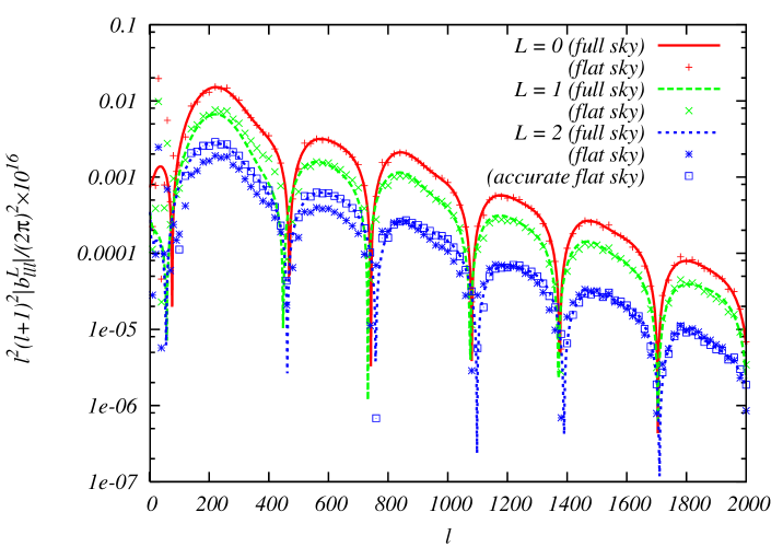
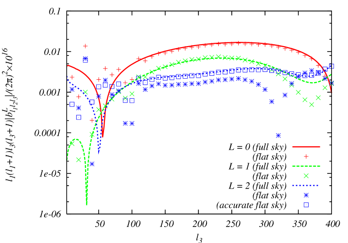
Figure 5: Absolute values of the CMB temperature reduced bispectra. The solid, long-dashed and short-dashed lines show the full-sky results for $L=0$, 1, and 2, respectively, while the plus, cross, and star symbols show the simplified flat-sky results from eq. (3.8) for $L=0$, 1, and 2, respectively. The square symbols show the original form of the flat-sky result for $L=2$ from eq. (3.3) before further approximation. (Top panel) Equilateral triangles, $|b_{\ell\ell\ell}^{L}|$. (Bottom panel) Squeezed triangles, $|b_{\ell_{1}\ell_{2}\ell_{3}}^{L}|$, with $\ell_{1}=\ell_{2}=200$, as a function of $\ell_{3}$.

Appendix B Analysis in the Sachs-Wolfe limit

As the calculations presented in section 3.2 are quite involved, some appropriate approximations would be useful for understanding the analytical structures of the basic results.

The Sachs–Wolfe limit, in which the radiation transfer function is given by ${\cal T}_{\ell}(k)\to-\frac{1}{5}j_{\ell}(kr_{*})$, provides such a convenient approximation. With this transfer function, $\alpha_{\ell}(r)$ (eq. 3.33) simplifies to $\alpha_{\ell}(r)\to-\frac{1}{5r_{*}^{2}}\delta(r-r_{*})$, where $r_{*}\equiv\tau_{0}-\tau_{*}$ is the conformal distance to the last scattering surface. Similarly, for a scale-invariant spectrum of $\zeta$, $P_{\zeta}(k)=\frac{2\pi^{2}}{k^{3}}A_{S}$, $\beta_{\ell}(r)$ (eq. 3.34) becomes

$$\beta_{\ell L}(r_{*})\to-\frac{\pi^{2}}{10}A_{S}\frac{\Gamma\left(\frac{\ell+L}{2}\right)}{\Gamma\left(\frac{\ell-L+3}{2}\right)\Gamma\left(\frac{-\ell+L+3}{2}\right)\Gamma\left(\frac{\ell+L+4}{2}\right)}~{},$$ (B.1)

where $\Gamma(x)$ is the Gamma function. Using these $\alpha_{\ell}$ and $\beta_{\ell}$ in eq. (3.32), one finds the Sachs–Wolfe approximation of the CMB bispectrum as

$$B_{\ell_{1}\ell_{2}\ell_{3}}^{L} \to -\frac{1}{5}\left[\prod_{n=1}^{3}\sum_{L_{n}}(-1)^{\frac{\ell_{n}+L_{n}}{2}}\right]I_{L_{1}L_{2}L_{3}}\beta_{\ell_{1}L_{1}}(r_{*})\beta_{\ell_{2}L_{2}}(r_{*})$$ (B.4)

$$\times\frac{4\pi}{2L+1}I_{\ell_{1}L_{1}L}I_{\ell_{2}L_{2}L}(-1)^{\ell_{2}+L_{1}}\delta_{L_{3},\ell_{3}}\left\{\begin{array}[]{ccc}\ell_{1}&\ell_{2}&\ell_{3}\\ L_{2}&L_{1}&L\end{array}\right\}+(\mbox{2 perm}).$$

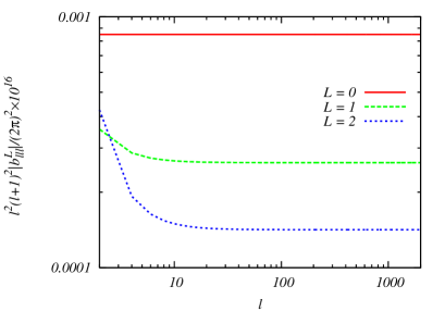
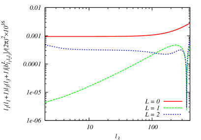
Figure 6: Absolute values of the CMB temperature reduced bispectra for $L=0$ (solid), 1 (long-dashed), and 2 (short-dashed), in the Sachs–Wolfe limit. (Left panel) Equilateral triangles, $|b_{\ell\ell\ell}^{L}|$. (Right panel) Squeezed triangles, $|b_{\ell_{1}\ell_{2}\ell_{3}}^{L}|$, with $\ell_{1}=\ell_{2}=200$, as a function of $\ell_{3}$.

Figure 6 shows the reduced CMB temperature bispectra in the Sachs–Wolfe limit. The basic behaviors, such as the monotonic decrease of the equilateral amplitudes as a function of $L$ and the suppression of the $L=1$ term in the squeezed limit, are all reproduced by the simple Sachs–Wolfe limit calculations. These results may be compared with figures 2 and 3.

Appendix C Full Fisher matrix

In section 3.3, we have presented the 1-$\sigma$ marginalized constraints on $c_{0}$, $c_{1}$, and $c_{2}$, assuming that only $c_{0}$ and one of $c_{1}$ and $c_{2}$ are varied simultaneously. In this appendix, we provide the full Fisher matrix, $F_{LL^{\prime}}$, involving all of $c_{0}$, $c_{1}$, and $c_{2}$, calculated up to $\ell_{\rm max}=2000$:

$$F_{LL^{\prime}}=\left(\begin{array}[]{ccc}5232&16.94&-5.986\\ 16.94&26.53&66.85\\ -5.986&66.85&618.1\end{array}\right)\times 10^{-5}~{}.$$ (C.4)

From this matrix, one can compute the cross-correlation coefficients, $r_{LL^{\prime}}\equiv F_{LL^{\prime}}/\sqrt{F_{LL}F_{L^{\prime}L^{\prime}}}$. We find $r_{01}=0.045$ and $r_{02}=-0.003$, indicating that $c_{0}$ and $c_{1}$ are nearly uncorrelated, so are $c_{0}$ and $c_{2}$. However, there is a high degree of correlation between $c_{1}$ and $c_{2}$: $r_{12}=0.522$. As a result, the marginalized error bars increase slightly to

$$(\delta c_{0},\delta c_{1},\delta c_{2})=\left(\sqrt{F^{-1}_{00}},\sqrt{F^{-1}_{11}},\sqrt{F^{-1}_{22}}\right)=(4.4,72,15)~{}.$$ (C.5)

References

- [1] P. Creminelli and M. Zaldarriaga, Single field consistency relation for the 3-point function, JCAP 0410 (2004) 006, [astro-ph/0407059].
- [2] E. Komatsu, N. Afshordi, N. Bartolo, D. Baumann, J. Bond, et. al., Non-Gaussianity as a Probe of the Physics of the Primordial Universe and the Astrophysics of the Low Redshift Universe, arXiv:0902.4759.
- [3] I. Agullo and L. Parker, Non-gaussianities and the Stimulated creation of quanta in the inflationary universe, Phys.Rev. D83 (2011) 063526, [arXiv:1010.5766].
- [4] J. Ganc, Calculating the local-type for slow-roll inflation with a non-vacuum initial state, Phys.Rev. D84 (2011) 063514, [arXiv:1104.0244].
- [5] D. Chialva, Signatures of very high energy physics in the squeezed limit of the bispectrum (violation of Maldacena’s condition), JCAP 1210 (2012) 037, [arXiv:1108.4203].
- [6] M. H. Namjoo, H. Firouzjahi, and M. Sasaki, Violation of non-Gaussianity consistency relation in a single field inflationary model, arXiv:1210.3692.
- [7] X. Chen, H. Firouzjahi, M. H. Namjoo, and M. Sasaki, A Single Field Inflation Model with Large Local Non-Gaussianity, arXiv:1301.5699.
- [8] E. Komatsu and D. N. Spergel, Acoustic signatures in the primary microwave background bispectrum, Phys.Rev. D63 (2001) 063002, [astro-ph/0005036].
- [9] G. Hinshaw, D. Larson, E. Komatsu, D. Spergel, C. Bennett, et. al., Nine-Year Wilkinson Microwave Anisotropy Probe (WMAP) Observations: Cosmological Parameter Results, arXiv:1212.5226.
- [10] Z. Hou, C. Reichardt, K. Story, B. Follin, R. Keisler, et. al., Constraints on Cosmology from the Cosmic Microwave Background Power Spectrum of the 2500-square degree SPT-SZ Survey, arXiv:1212.6267.
- [11] J. L. Sievers, R. A. Hlozek, M. R. Nolta, V. Acquaviva, G. E. Addison, et. al., The Atacama Cosmology Telescope: Cosmological parameters from three seasons of data, arXiv:1301.0824.
- [12] D. Babich, P. Creminelli, and M. Zaldarriaga, The Shape of non-Gaussianities, JCAP 0408 (2004) 009, [astro-ph/0405356].
- [13] J. M. Maldacena, Non-Gaussian features of primordial fluctuations in single field inflationary models, JHEP 0305 (2003) 013, [astro-ph/0210603].
- [14] C. Bennett, D. Larson, J. Weiland, N. Jarosik, G. Hinshaw, et. al., Nine-Year Wilkinson Microwave Anisotropy Probe (WMAP) Observations: Final Maps and Results, arXiv:1212.5225.
- [15] T. Okamoto and W. Hu, The angular trispectra of CMB temperature and polarization, Phys.Rev. D66 (2002) 063008, [astro-ph/0206155].
- [16] N. Kogo and E. Komatsu, Angular trispectrum of cmb temperature anisotropy from primordial non-gaussianity with the full radiation transfer function, Phys.Rev. D73 (2006) 083007, [astro-ph/0602099].
- [17] L. Boubekeur and D. Lyth, Detecting a small perturbation through its non-Gaussianity, Phys.Rev. D73 (2006) 021301, [astro-ph/0504046].
- [18] T. Suyama and M. Yamaguchi, Non-Gaussianity in the modulated reheating scenario, Phys.Rev. D77 (2008) 023505, [arXiv:0709.2545].
- [19] E. Komatsu, Hunting for Primordial Non-Gaussianity in the Cosmic Microwave Background, Class.Quant.Grav. 27 (2010) 124010, [arXiv:1003.6097].
- [20] N. S. Sugiyama, E. Komatsu, and T. Futamase, Non-Gaussianity Consistency Relation for Multi-field Inflation, Phys.Rev.Lett. 106 (2011) 251301, [arXiv:1101.3636].
- [21] K. M. Smith, M. LoVerde, and M. Zaldarriaga, A universal bound on N-point correlations from inflation, Phys.Rev.Lett. 107 (2011) 191301, [arXiv:1108.1805].
- [22] A. Lewis, The real shape of non-Gaussianities, JCAP 1110 (2011) 026, [arXiv:1107.5431].
- [23] J. Bramante and J. Kumar, Local Scale-Dependent Non-Gaussian Curvature Perturbations at Cubic Order, JCAP 1109 (2011) 036, [arXiv:1107.5362].
- [24] N. S. Sugiyama, Consistency Relation for multifield inflation scenario with all loop contributions, JCAP 1205 (2012) 032, [arXiv:1201.4048].
- [25] V. Assassi, D. Baumann, and D. Green, On Soft Limits of Inflationary Correlation Functions, JCAP 1211 (2012) 047, [arXiv:1204.4207].
- [26] M. Shiraishi, D. Nitta, S. Yokoyama, and K. Ichiki, Optimal limits on primordial magnetic fields from CMB temperature bispectrum of passive modes, JCAP 1203 (2012) 041, [arXiv:1201.0376].
- [27] M. Shiraishi, Parity violation of primordial magnetic fields in the CMB bispectrum, JCAP 1206 (2012) 015, [arXiv:1202.2847].
- [28] N. Barnaby, R. Namba, and M. Peloso, Observable non-gaussianity from gauge field production in slow roll inflation, and a challenging connection with magnetogenesis, Phys.Rev. D85 (2012) 123523, [arXiv:1202.1469].
- [29] N. Bartolo, S. Matarrese, M. Peloso, and A. Ricciardone, The anisotropic power spectrum and bispectrum in the mechanism, arXiv:1210.3257.
- [30] S. Endlich, A. Nicolis, and J. Wang, Solid Inflation, arXiv:1210.0569.
- [31] M. Liguori, F. Hansen, E. Komatsu, S. Matarrese, and A. Riotto, Testing primordial non-gaussianity in cmb anisotropies, Phys.Rev. D73 (2006) 043505, [astro-ph/0509098].
- [32] D. M. Goldberg and D. N. Spergel, Microwave background bispectrum. 2. A probe of the low redshift universe, Phys.Rev. D59 (1999) 103002, [astro-ph/9811251].
- [33] L. Boubekeur, P. Creminelli, G. D’Amico, J. Norena, and F. Vernizzi, Sachs-Wolfe at second order: the CMB bispectrum on large angular scales, JCAP 0908 (2009) 029, [arXiv:0906.0980].
- [34] A. Lewis, A. Challinor, and D. Hanson, The shape of the CMB lensing bispectrum, JCAP 1103 (2011) 018, [arXiv:1101.2234].
- [35] C. T. Byrnes, S. Nurmi, G. Tasinato, and D. Wands, Scale dependence of local , JCAP 1002 (2010) 034, [arXiv:0911.2780].
- [36] C. T. Byrnes, M. Gerstenlauer, S. Nurmi, G. Tasinato, and D. Wands, Scale-dependent non-Gaussianity probes inflationary physics, JCAP 1010 (2010) 004, [arXiv:1007.4277].
- [37] S. Shandera, N. Dalal, and D. Huterer, A generalized local ansatz and its effect on halo bias, JCAP 1103 (2011) 017, [arXiv:1010.3722].
- [38] C. T. Byrnes and J.-O. Gong, General formula for the running of , Phys.Lett. B718 (2013) 718–721, [arXiv:1210.1851].
- [39] J. Ganc and E. Komatsu, Scale-dependent bias of galaxies and mu-type distortion of the cosmic microwave background spectrum from single-field inflation with a modified initial state, Phys.Rev. D86 (2012) 023518, [arXiv:1204.4241].
- [40] I. Agullo and S. Shandera, Large non-Gaussian Halo Bias from Single Field Inflation, JCAP 1209 (2012) 007, [arXiv:1204.4409].
- [41] F. Schmidt and L. Hui, Cosmic Microwave Background Power Asymmetry from Non-Gaussian Modulation, Phys.Rev.Lett. 110 (2013) 011301.
- [42] P. D. Meerburg, J. P. van der Schaar, and P. S. Corasaniti, Signatures of Initial State Modifications on Bispectrum Statistics, JCAP 0905 (2009) 018, [arXiv:0901.4044].
- [43] P. Kronberg, M. Bernet, F. Miniati, S. Lilly, M. Short, et. al., A Global Probe of Cosmic Magnetic Fields to High Redshifts, Astrophys.J. 676 (2008) 7079, [arXiv:0712.0435].
- [44] M. L. Bernet, F. Miniati, S. J. Lilly, P. P. Kronberg, and M. Dessauges-Zavadsky, Strong magnetic fields in normal galaxies at high redshifts, Nature 454 (2008) 302–304, [arXiv:0807.3347].
- [45] A. M. Wolfe, R. A. Jorgenson, T. Robishaw, C. Heiles, and J. X. Prochaska, An 84 microGauss Magnetic Field in a Galaxy at Redshift z=0.692, Nature 455 (2008) 638, [arXiv:0811.2408].
- [46] A. Fletcher, R. Beck, A. Shukurov, E. Berkhuijsen, and C. Horellou, Magnetic fields and spiral arms in the galaxy M51, arXiv:1001.5230.
- [47] A. Neronov and I. Vovk, Evidence for strong extragalactic magnetic fields from Fermi observations of TeV blazars, Science 328 (2010) 73–75, [arXiv:1006.3504].
- [48] K. Dolag, M. Kachelriess, S. Ostapchenko, and R. Tomas, Lower limit on the strength and filling factor of extragalactic magnetic fields, Astrophys.J. 727 (2011) L4, [arXiv:1009.1782].
- [49] F. Tavecchio, G. Ghisellini, L. Foschini, G. Bonnoli, G. Ghirlanda, et. al., The intergalactic magnetic field constrained by Fermi/LAT observations of the TeV blazar 1ES 0229+200, Mon.Not.Roy.Astron.Soc. 406 (2010) L70–L74, [arXiv:1004.1329].
- [50] K. Takahashi, M. Mori, K. Ichiki, and S. Inoue, Lower Bounds on Intergalactic Magnetic Fields from Simultaneously Observed GeV-TeV Light Curves of the Blazar Mrk 501, arXiv:1103.3835.
- [51] S. Kanno, J. Soda, and M.-a. Watanabe, Cosmological Magnetic Fields from Inflation and Backreaction, JCAP 0912 (2009) 009, [arXiv:0908.3509].
- [52] V. Demozzi, V. Mukhanov, and H. Rubinstein, Magnetic fields from inflation?, JCAP 0908 (2009) 025, [arXiv:0907.1030].
- [53] V. Demozzi and C. Ringeval, Reheating constraints in inflationary magnetogenesis, JCAP 1205 (2012) 009, [arXiv:1202.3022].
- [54] T. Suyama and J. Yokoyama, Metric perturbation from inflationary magnetic field and generic bound on inflation models, Phys.Rev. D86 (2012) 023512, [arXiv:1204.3976].
- [55] T. Fujita and S. Mukohyama, Universal upper limit on inflation energy scale from cosmic magnetic field, JCAP 1210 (2012) 034, [arXiv:1205.5031].
- [56] T. S. Koivisto and F. R. Urban, Three-magnetic fields, Phys.Rev. D85 (2012) 083508, [arXiv:1112.1356].
- [57] F. R. Urban and T. K. Koivisto, Perturbations and non-Gaussianities in three-form inflationary magnetogenesis, JCAP 1209 (2012) 025, [arXiv:1207.7328].
- [58] R. Durrer, T. Kahniashvili, and A. Yates, Microwave background anisotropies from Alfven waves, Phys.Rev. D58 (1998) 123004, [astro-ph/9807089].
- [59] A. Mack, T. Kahniashvili, and A. Kosowsky, Microwave background signatures of a primordial stochastic magnetic field, Phys.Rev. D65 (2002) 123004, [astro-ph/0105504].
- [60] A. Lewis, CMB anisotropies from primordial inhomogeneous magnetic fields, Phys.Rev. D70 (2004) 043011, [astro-ph/0406096].
- [61] D. G. Yamazaki, K. Ichiki, T. Kajino, and G. J. Mathews, Effects of a Primordial Magnetic Field on Low and High Multipoles of the CMB, Phys.Rev. D77 (2008) 043005, [arXiv:0801.2572].
- [62] D. Paoletti, F. Finelli, and F. Paci, The full contribution of a stochastic background of magnetic fields to CMB anisotropies, Mon.Not.Roy.Astron.Soc. 396 (2009) 523–534, [arXiv:0811.0230].
- [63] F. Finelli, F. Paci, and D. Paoletti, The Impact of Stochastic Primordial Magnetic Fields on the Scalar Contribution to Cosmic Microwave Background Anisotropies, Phys.Rev. D78 (2008) 023510, [arXiv:0803.1246].
- [64] J. R. Shaw and A. Lewis, Massive Neutrinos and Magnetic Fields in the Early Universe, Phys.Rev. D81 (2010) 043517, [arXiv:0911.2714].
- [65] J. R. Shaw and A. Lewis, Constraining Primordial Magnetism, Phys.Rev. D86 (2012) 043510, [arXiv:1006.4242].
- [66] D. Paoletti and F. Finelli, CMB Constraints on a Stochastic Background of Primordial Magnetic Fields, Phys.Rev. D83 (2011) 123533, [arXiv:1005.0148].
- [67] D. Paoletti and F. Finelli, Constraints on a Stochastic Background of Primordial Magnetic Fields with WMAP and South Pole Telescope data, arXiv:1208.2625.
- [68] A. P. Yadav, L. Pogosian, and T. Vachaspati, Probing Primordial Magnetism with Off-Diagonal Correlators of CMB Polarization, arXiv:1207.3356.
- [69] M. Shiraishi, S. Saga, and S. Yokoyama, CMB power spectra induced by primordial cross-bispectra between metric perturbations and vector fields, JCAP 1211 (2012) 046, [arXiv:1209.3384].
- [70] K. E. Kunze, Cross correlations from back reaction on stochastic magnetic fields, JCAP 1302 (2013) 009, [arXiv:1209.4570].
- [71] K. E. Kunze, CMB and matter power spectra from cross correlations of primordial curvature and magnetic fields, arXiv:1301.6105.
- [72] T. Seshadri and K. Subramanian, CMB bispectrum from primordial magnetic fields on large angular scales, Phys.Rev.Lett. 103 (2009) 081303, [arXiv:0902.4066].
- [73] C. Caprini, F. Finelli, D. Paoletti, and A. Riotto, The cosmic microwave background temperature bispectrum from scalar perturbations induced by primordial magnetic fields, JCAP 0906 (2009) 021, [arXiv:0903.1420].
- [74] P. Trivedi, K. Subramanian, and T. Seshadri, Primordial Magnetic Field Limits from Cosmic Microwave Background Bispectrum of Magnetic Passive Scalar Modes, Phys.Rev. D82 (2010) 123006, [arXiv:1009.2724].
- [75] R.-G. Cai, B. Hu, and H.-B. Zhang, Acoustic signatures in the Cosmic Microwave Background bispectrum from primordial magnetic fields, JCAP 1008 (2010) 025, [arXiv:1006.2985].
- [76] M. Shiraishi, D. Nitta, S. Yokoyama, K. Ichiki, and K. Takahashi, Cosmic microwave background bispectrum of vector modes induced from primordial magnetic fields, Phys.Rev. D82 (2010) 121302, [arXiv:1009.3632].
- [77] M. Shiraishi, D. Nitta, S. Yokoyama, K. Ichiki, and K. Takahashi, Computation approach for CMB bispectrum from primordial magnetic fields, Phys.Rev. D83 (2011) 123523, [arXiv:1101.5287].
- [78] M. Shiraishi, D. Nitta, S. Yokoyama, K. Ichiki, and K. Takahashi, Cosmic microwave background bispectrum of tensor passive modes induced from primordial magnetic fields, Phys.Rev. D83 (2011) 123003, [arXiv:1103.4103].
- [79] C. Caprini, R. Durrer, and T. Kahniashvili, The Cosmic microwave background and helical magnetic fields: The Tensor mode, Phys.Rev. D69 (2004) 063006, [astro-ph/0304556].
- [80] M. Shiraishi, D. Nitta, and S. Yokoyama, Parity Violation of Gravitons in the CMB Bispectrum, Prog.Theor.Phys. 126 (2011) 937–959, [arXiv:1108.0175].
- [81] A. R. Pullen and M. Kamionkowski, Cosmic Microwave Background Statistics for a Direction-Dependent Primordial Power Spectrum, Phys.Rev. D76 (2007) 103529, [arXiv:0709.1144].
- [82] Y.-Z. Ma, G. Efstathiou, and A. Challinor, Testing a direction-dependent primordial power spectrum with observations of the Cosmic Microwave Background, Phys.Rev. D83 (2011) 083005, [arXiv:1102.4961].
- [83] B. Ratra, Cosmological ’seed’ magnetic field from inflation, Astrophys.J. 391 (1992) L1–L4.
- [84] J. Martin and J. Yokoyama, Generation of Large-Scale Magnetic Fields in Single-Field Inflation, JCAP 0801 (2008) 025, [arXiv:0711.4307].
- [85] R. R. Caldwell, L. Motta, and M. Kamionkowski, Correlation of inflation-produced magnetic fields with scalar fluctuations, Phys.Rev. D84 (2011) 123525, [arXiv:1109.4415].
- [86] L. Motta and R. R. Caldwell, Non-Gaussian features of primordial magnetic fields in power-law inflation, Phys.Rev. D85 (2012) 103532, [arXiv:1203.1033].
- [87] R. K. Jain and M. S. Sloth, A Magnetic Consistency Relation, arXiv:1207.4187.
- [88] R. K. Jain and M. S. Sloth, On the non-Gaussian correlation of the primordial curvature perturbation with vector fields, arXiv:1210.3461.
- [89] D. Seery, Magnetogenesis and the primordial non-gaussianity, JCAP 0908 (2009) 018, [arXiv:0810.1617].
- [90] A. A. Starobinsky, Stochastic De Sitter (inflationary) Stage In The Early Universe, Field heory, Quantum Gravity and Strings (1986) 107–126.
- [91] I. Affleck and M. Dine, A New Mechanism for Baryogenesis, Nucl.Phys. B249 (1985) 361.
- [92] D. H. Lyth and D. Wands, Generating the curvature perturbation without an inflaton, Phys.Lett. B524 (2002) 5–14, [hep-ph/0110002].
- [93] T. R. Dulaney and M. I. Gresham, Primordial Power Spectra from Anisotropic Inflation, Phys.Rev. D81 (2010) 103532, [arXiv:1001.2301].
- [94] A. Gumrukcuoglu, B. Himmetoglu, and M. Peloso, Scalar-Scalar, Scalar-Tensor, and Tensor-Tensor Correlators from Anisotropic Inflation, Phys.Rev. D81 (2010) 063528, [arXiv:1001.4088].
- [95] M.-a. Watanabe, S. Kanno, and J. Soda, The Nature of Primordial Fluctuations from Anisotropic Inflation, Prog.Theor.Phys. 123 (2010) 1041–1068, [arXiv:1003.0056].
- [96] M.-a. Watanabe, S. Kanno, and J. Soda, Inflationary Universe with Anisotropic Hair, Phys.Rev.Lett. 102 (2009) 191302, [arXiv:0902.2833].
- [97] M. Shiraishi and S. Yokoyama, Violation of the Rotational Invariance in the CMB Bispectrum, Prog.Theor.Phys. 126 (2011) 923–935, [arXiv:1107.0682].
- [98] N. Bartolo, E. Dimastrogiovanni, M. Liguori, S. Matarrese, and A. Riotto, An Estimator for statistical anisotropy from the CMB bispectrum, JCAP 1201 (2012) 029, [arXiv:1107.4304].
- [99] R. Emami and H. Firouzjahi, Curvature Perturbations in Anisotropic Inflation with Symmetry Breaking, arXiv:1301.1219.
- [100] K. Dimopoulos, M. Karciauskas, and J. M. Wagstaff, Vector Curvaton without Instabilities, Phys.Lett. B683 (2010) 298–301, [arXiv:0909.0475].
- [101] R. Namba, Curvature Perturbations from a Massive Vector Curvaton, Phys.Rev. D86 (2012) 083518, [arXiv:1207.5547].
- [102] H. Funakoshi and K. Yamamoto, Primordial bispectrum from inflation with background gauge fields, arXiv:1212.2615.
- [103] S. Yokoyama and J. Soda, Primordial statistical anisotropy generated at the end of inflation, JCAP 0808 (2008) 005, [arXiv:0805.4265].
- [104] A. Gruzinov, Elastic inflation, Phys.Rev. D70 (2004) 063518, [astro-ph/0404548].
- [105] M. Shiraishi, S. Yokoyama, K. Ichiki, and K. Takahashi, Analytic formulae of the CMB bispectra generated from non-Gaussianity in the tensor and vector perturbations, Phys.Rev. D82 (2010) 103505, [arXiv:1003.2096].
- [106] M. Shiraishi, D. Nitta, S. Yokoyama, K. Ichiki, and K. Takahashi, CMB Bispectrum from Primordial Scalar, Vector and Tensor non-Gaussianities, Prog.Theor.Phys. 125 (2011) 795–813, [arXiv:1012.1079].
- [107] Y. Rodriguez, J. P. B. Almeida, and C. A. Valenzuela-Toledo, The different varieties of the Suyama-Yamaguchi consistency relation and its violation as a signal of statistical inhomogeneity, arXiv:1301.5843.
- [108] M. Shiraishi, S. Yokoyama, K. Ichiki, and T. Matsubara, Scale-dependent bias due to primordial vector field, arXiv:1301.2778.
- [109] M. Peloso and M. Pietroni, Galilean invariance and the consistency relation for the nonlinear squeezed bispectrum of large scale structure, arXiv:1302.0223.
- [110] A. Kehagias and A. Riotto, Symmetries and Consistency Relations in the Large Scale Structure of the Universe, arXiv:1302.0130.
- [111] Planck Collaboration Collaboration, P. Ade et. al., Planck 2013 Results. XXIV. Constraints on primordial non-Gaussianity, arXiv:1303.5084.