CSSM Lattice Collaboration
Structure and Flow of the Nucleon Eigenstates in Lattice QCD
Abstract
A determination of the excited energy eigenstates of the nucleon, , , , is presented in full QCD using flavor PACS-CS gauge configurations. The correlation-matrix method is used and is built using standard nucleon interpolators employing smearings at the fermion sources and sinks. We develop and demonstrate a new technique that allows the eigenvectors obtained to be utilized to track the propagation of the intrinsic nature of energy-states from one quark mass to the next. This approach is particularly useful for larger dimension correlation matrices where more near-degenerate energy-states can appear in the spectrum.
pacs:
11.15.Ha,12.38.Gc,12.38.-tI Introduction
Resonances represent some of the rich dynamics of one of the fundamental interactions of Nature, the strong interaction of quarks and gluons. Lattice QCD is the only ab initio first principles approach to the fundamental quantum field theory governing the properties of hadrons and ultimately we wish to test our theoretical understanding of resonances against their experimentally determined properties.
From lattice QCD, the ground-state hadron spectrum is now relatively well understood Durr et al. (2008). However, gaining knowledge of the excited-state spectrum on the lattice presents additional challenges, as the excited energy-states are extracted from the sub-leading exponentials of the correlation functions. A determination of the excited state energy spectrum, including multi-particle states, requires significant effort and some progress is now being made. We can expect the interplay between lattice QCD predictions and experimental measurement to be very productive in the coming years.
In the case of nucleon resonances, the first positive parity excitation of the nucleon, the or Roper resonance, has been a subject of considerable interest since its discovery in 1964 through a partial-wave analysis of pion-nucleon scattering data Roper (1964). This state has a surprisingly low mass, which is well below the first negative parity excitation. In constituent quark models with a harmonic oscillator potential this state (with principal quantum number ) appears above the lowest-lying odd-parity (1535) state Isgur and Karl (1977, 1979), whereas in Nature the Roper resonance is almost 100 MeV below the state. This presents a phenomenological challenge to our understanding of level ordering. Similar difficulties occur with the and resonances. Due to its surprisingly low mass, the state has lead to enormous curiosity and much speculation about its nature. For example, the Roper resonance has been described as a hybrid baryon with explicitly excited gluon field configurations Li et al. (1992); Carlson and Mukhopadhyay (1991), or as a breathing mode of the ground state Guichon (1985) or as a five quark (meson-baryon) state Krehl et al. (2000). Significant resources have been devoted in the past from the lattice QCD perspective to find the elusive low-lying Roper state, in both quenched Allton et al. (1993); Lee and Leinweber (1999); Gockeler et al. (2002); Sasaki et al. (2002); Melnitchouk et al. (2003); Edwards et al. (2003); Lee et al. (2003); Brommel et al. (2004); Mathur et al. (2005); Sasaki (2003); Burch et al. (2004); Basak et al. (2007); Mahbub et al. (2009a, b); Fleming et al. (2009); Mahbub et al. (2010a, b) and in full Bulava et al. (2009); Engel et al. (2010); Edwards et al. (2011); Mahbub et al. (2012); Lin and Cohen (2011) QCD.
The ‘Variational method’ Michael (1985); Luscher and Wolff (1990) is the state-of-the-art approach for determining the excited state hadron spectrum. It is based on the creation of a matrix of correlation functions in which different superpositions of excited-state contributions are linearly combined to isolate the energy eigenstates. A low-lying Roper state was identified with this method using a variety of source and sink smearings in constructing correlation matrices Mahbub et al. (2009b, 2010a) in quenched QCD. Recent developments of algorithms and computational power have enabled the extension to full QCD. Some full QCD analyses using the variational method can be found in Refs. Bulava et al. (2009); Lin et al. (2009); Engel et al. (2010); Edwards et al. (2011); Bulava et al. (2010); Mahbub et al. (2012); Morningstar et al. (2011); Bulava (2011); Menadue et al. (2011); Edwards et al. (2012); Engel et al. (2013). Here we consider the techniques of Refs. Mahbub et al. (2009b, 2010a) to explore the low-lying even- and odd- parity states of the nucleon using 2+1-flavor dynamical QCD gauge-field configurations from the PACS-CS collaboration Aoki et al. (2009). A small subset of the results presented here have appeared in Refs. Mahbub et al. (2012, 2013).
The number of energy states revealed in the correlation matrix method depends on the number of unique operators chosen which have the quantum numbers of the desired states. Hence, a clear identification of these states is necessary to observe changes in these energy-states as a function of quark mass, in principle to the physical quark mass. This allows the quark mass dependence and structure of the extracted energy eigenstates to be explored systematically. The new technique that we develop here can be used when any parameter of the theory is varied to explore how the nature of the states and energies change with that parameter.
The principal focus of this paper is to present the details of our eigenvector analysis to track the states from the heavy to the light quark mass region. In doing so, we consider the states to illustrate the utility of the method. The operator basis is increased with the use of fermion source and sink smearings as in Ref. Mahbub et al. (2012). Then, the propagation of the energy states are presented after analyzing the state of eigenvectors at adjacent quarks masses. Results are presented for both the non-symmetric and symmetric eigenvalue equations, and these are compared and related to each other.
In this analysis, we haven’t been able to isolate the multi-particle thresholds at our three light quark masses. We proceed under the assumption that the couplings to these 5+ quark states have relatively small overlap with our 3-quark interpolators and that the effective mass functions are largely unaffected by multi-particle states with small couplings to our interpolators. To monitor this we use the full covariance-matrix based in order to accurately assess the extent to which our effective mass function plateau is associated with a single state. Ultimately, in addition to the 3-quark operators, one needs to include 5- or 7- or more- quark operators Morningstar et al. (2011); Lang and Verduci (2012); Morningstar et al. (2013) in the correlation matrix to extract all the states in the spectrum.
If we denote the dimensionality of the Hilbert space of the lattice Hamiltonian to be , then in an ideal world we would select linearly independent operators to construct our correlation matrix with sufficient statistical accuracy and then diagonalize this to obtain the exact energy eigenstates for this lattice Hamiltonian. Obviously and unfortunately this is not computationally feasible on any realistic lattice and the best that we can do is choose a relatively small number of operators, , where . If we choose these operator interpolating fields wisely, then the subspace they span will have good overlap with the subspace spanned by the lowest eigenstates of the Hamiltonian. If this is the case then with sufficient statistics we can hope to extract good estimates of the lowest energy states. If we observe, for example, that adding additional operators to increase to reveals new low-lying states, then clearly we had not chosen our operators wisely enough. The test of whether or not we have revealed all of the lowest states of the lattice Hamiltonian is that the process of adding additional and new operators does not reveal new low-lying excited states. We present a clearer and more complete discussion of these issues in the Appendix.
The linear independence of additional operators can be judged by monitoring the condition number of the correlation matrix. If the condition number does not increase significantly when an operator is added then the additional operator enhances the basis in a sufficiently independent manner.
The paper is arranged as follows: Section II contains a standard description of the mass extraction from a two-point correlation function with a brief introduction of Gaussian smearings at the fermion sources. The variational method is presented in section III followed by simulation details in section IV. Section V contains a discussion of the energy eigenstates identification. Results for the flow of eigenvectors are presented in section VI followed by concluding remarks in section VII. Finally, a pedagogical discussion of the correlation matrix is presented in Appendix in terms of the lattice Hamiltonian.
II Energy States from Two-point Correlation Functions
A two point correlation function can be written as
| (1) |
where the Dirac spin indices are implicit. The operator creates states from the vacuum at space-time point and, following the evolution of the states in Euclidean time , the states are destroyed by the operator at the point . indicates the time ordering of the operators.
The energy eigenstates of hadrons are extracted using operators suitably chosen to have overlap with the desired states of interest. If we consider a baryon state , then a complete set of momentum eigenstates provides,
| (2) |
where can also include multi-particle states that the operator couples with. The substitution of Eq. (2) into Eq. (1) yields
| (3) |
Using the translational operator, the operator can be expressed as
| (4) |
where is the lattice Hamiltonian and is the momentum operator whose eigenvalue is the total momentum of the system. Inserting this into Eq. (3) we obtain
| (5) |
The overlap of the interpolating fields and with positive and negative parity baryon states can be parametrized by a complex quantity called the coupling strength, , which can be defined for positive parity states by
| (6) |
| (7) |
For the negative parity states one requires
| (8) |
| (9) |
Here, and are the couplings of the interpolating functions at the sink and the source respectively and is the mass of the state . is the energy of the state , where . Therefore, mass of a energy-state is obtained with the momentum projection of the correlation function at .
The standard spin sums may now be performed. For the positive parity hadron states, this can be expressed as
| (10) |
and for the negative parity states, one encounters
| (11) |
By substituting the above Eqs. for the positive and negative parity states in Eq. (5) we obtain,
| (12) |
At momentum , , and a parity projection operator can be introduced,
| (13) |
We can isolate the masses of the even and odd parity energy-states by taking the trace of with the operators and . The positive parity states propagate through the and elements of the Dirac matrix, whereas, negative parity states propagate through the and elements. The correlation function for positive and negative parity states can then be written as
| (14) |
The correlation function contains a superposition of energy-states, i.e. both ground and excited energy-states. The mass of the lowest energy-state, can be extracted at large where the contributions from all other excited-states are suppressed,
| (15) |
where, and are now couplings of interpolators to the lowest energy-state.
II.1 Source Smearing
The spatial fermion source-smearing Gusken (1990) technique is applied to increase the overlap of the interpolators with the lower lying states. We employ a fixed boundary condition in the time direction for the fermions by setting in the hopping terms of the fermion action with periodic boundary conditions imposed in the spatial directions. Gauge invariant Gaussian smearing Gusken (1990) in the spatial dimensions is applied through an iterative process. The smearing procedure is:
| (16) |
where,
| (17) |
where the parameter is used in our calculation. After repeating the procedures times on a point source the resulting smeared fermion field is,
| (18) |
III Variational Method
The extraction of the ground state mass can be done straightforwardly using Eq. (15). However access to the excited state masses requires additional effort due to the presence of these energy-states at the sub-leading of the exponential. Here we consider the variational method Michael (1985); Luscher and Wolff (1990), which allows for a variety of superpositions of excited-states in its cross-correlation discussed below.
The variational method requires the cross correlation of operators so that the operator space can be diagonalised and the excited state masses extracted from the exponential nature of the diagonalised basis. To access states of the spectrum, one requires a minimum of interpolators. With the assumption that only states contribute significantly to at time , the parity projected two point correlation function matrix for can be written as
| (19) |
where Dirac indices are implicit. Here, and are the couplings of interpolators and at the sink and source respectively to eigenstates and is the mass of the energy-state . The use of identical source and sink interpolators provides and then in the ensemble average is a Hermitian matrix, i.e. . Moreover, considering both and configurations makes a real symmetric matrix. The interpolators have the same quantum numbers and provide an -dimensional basis upon which to describe the states. Using this basis we aim to construct independent interpolating source and sink fields which isolate baryon states i.e.
| (20) |
| (21) |
such that,
| (22) |
| (23) |
where and are the coupling strengths of and to the state . Consider a real eigenvector which operates on the correlation matrix from the right, one can obtain,
| (24) |
For notational convenience, in the remainder of the discussion the repeated indices are to be understood as being summed over, whereas, , which stands for a particular state, is not.
In the ensemble average, . Therefore, considering provides an improved unbiased estimator and enables the use a symmetric eigenvalue equation as discussed below. To ensure that the matrix elements are all , each element of is normalized by (discussed in the Appendix).
In Eq. (24), since the only dependence comes from the exponential term, we can write a recurrence relation at time as,
| (25) |
for sufficiently large and Blossier et al. (2009); Mahbub et al. (2009a).
Multiplying the above equation by from the left we get,
| (26) |
This is an eigenvalue equation for eigenvector with eigenvalue . We can also solve the left eigenvalue equation to recover the eigenvector,
| (27) |
Similarly,
| (28) |
Since is a real symmetric matrix . The vectors and diagonalize the correlation matrix at time and making the projected correlation matrix,
| (29) |
The parity projected, eigenstate projected correlator,
| (30) |
is then used to obtain masses of different states. We construct the effective mass function
| (31) |
and apply standard analysis techniques as described in Ref. Mahbub et al. (2009a).
Since , we can rewrite Eq. (26)as
Multiplying from the left by provides
and defining,
| (32) |
we find
| (33) |
(also shown in Eq. (64)). We note the matrix
| (34) |
is real symmetric, with the same eigenvalue and with the orthogonal to each other. If we had not used the sum then the matrix in Eq. (34) would be hermitian and hence would still have real eigenvalues and orthogonal eigenvectors. The coefficients of interpolators creating an energy eigenstate is recovered by
| (35) |
IV Simulation parameters
PACS-CS flavor dynamical-fermion configurations Aoki et al. (2009) made available through the ILDG Beckett et al. (2011) are used. These configurations use the non-perturbatively -improved Wilson fermion action and the Iwasaki-gauge action Iwasaki (1983). The lattice volume is , with providing a lattice spacing fm and lattice volume of .
The degenerate up and down quark masses are considered, with the hopping parameter values of corresponding to pion masses of = 0.702, 0.572, 0.413, 0.293, 0.156 GeV Aoki et al. (2009); for the strange quark . We consider an ensemble of 350 configurations each for the four heavier quarks mass and 198 configurations for the lightest quark. An ensemble of 750 samples for the lightest quark mass is created by using well separated multiple fermion sources on each configuration. We use the jackknife method to calculate the error, where the for projected correlator fits is obtained via a covariance matrix analysis.
The complete set of local interpolating fields for the spin- nucleon are considered herein. Three different spin-flavor combinations of nucleon interpolators are considered,
| (36) | ||||
| (37) | ||||
| (38) |
The and interpolators are used in Refs. Leinweber et al. (1991); Sasaki et al. (2002); Leinweber (1995). The interpolator is the time component of the local spin- isospin- interpolator which also couples to spin- states used, for instance, in Refs. Brommel et al. (2004); Zanotti et al. (2003); Mahbub et al. (2009a).
The local scalar-diquark nucleon interpolator, , is well known to have a good overlap with the ground state of the nucleon. Also, this interpolator is able to extract a low-lying Roper state in quenched QCD Mahbub et al. (2010a). On the other hand, the interpolator has pseudoscalar-diquark structure in the nucleon, which vanishes in the non-relativistic limit, couples strongly to higher energy states. Each interpolator has a unique Dirac structure giving rise to different spin-flavor combinations. Moreover, as each spinor has upper and lower components, with the lower components containing an implicit derivative, different combinations of zero, one, two and three derivative interpolators are provided.
The correlation matrices are constructed using different levels of gauge-invariant Gaussian smearing Gusken (1990) at the fermion sources and sinks Mahbub et al. (2012). A basis of smearing-sweep counts of 16, 35, 100 and 200 is selected following the extensive analysis of Ref. Mahbub et al. (2012).
It is important to consider the condition number for these matrices in order to examine the quality of our operator basis. We consider the normalized correlation matrix, , with made Hermition as discussed in Sec. III.
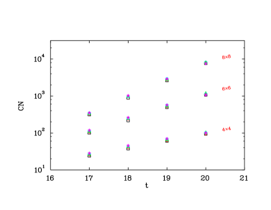
The condition numbers for our correlation matrices are illustrated in Fig. 1. We examine the change in the condition number for matrices composed of and as additional source smearings are introduced. We consider two levels of smearing in the matrix, three levels of smearing in the matrix and all four levels of smearing in the matrix.
Results for the five quark masses under consideration are provided. The tight clustering of the condition number for the wide range of quark masses considered indicates that the basis selected is appropriate for all these masses.
The condition numbers are displayed as a function of Euclidean time following the fermion source at . At early times, the different superposition of large excited state contributions gives rise to a relatively small condition number. However as these states become exponentially suppressed at larger Euclidean times, the condition number increases. If one waits to very large Euclidean times, all excitations are suppressed and all operators produce the same ground state rendering the condition number infinite. This will be realised for any basis set having overlap with the ground state. Thus it is important to conduct the correlation matrix analysis at times where excited states are present and the number of significant state contributions matches the size of the basis.
While the condition number increases as the smearing basis is enhanced, the condition number is the order of for our preferred variational analysis time of . This value is small relative to associated with standard double precision calculations.
Thus, the utilization of different fermion smearings at the source and the sink is an effective approach to enlarging the basis of operators. Our selection of smearing levels was based on the excited-state contributions observed in smeared-source to point-sink correlators Mahbub et al. (2012). By selecting smearing levels that provided well separated effective masses at early Euclidean times, we ensured that each operator was sufficiently independent, thus giving rise to an acceptable condition number for the correlation matrix.
V Eigenstates Identification
Let us consider interpolating fields making an parity-projected correlation matrix . In solving the generalized eigenvalue equations of Eqs. (26) and (28) we encounter the real and approximately symmetric matrices and , with the left and right eigenvectors and respectively. Thus the eigenvectors of these matrices are expected to be approximately orthogonal (left table in Table 1). As explained in the Appendix, the reason we have only approximate symmetry is that does not commute with itself at different times. This results because . The more closely the subspace spanned by our operators aligns with the subspace of the lowest energy eigenstates of , the less violation of symmetry there will be. If we do not use the sum, then all of the same arguments hold but with hermitian matrices.
This feature enables the use of the generalised measure
| (39) |
for the eigenvector , for example. This correlates eigenvectors at different quark masses and may be useful in tracking states.
In contrast, as already discussed, the matrix in Eq. (34) is symmetric, hence the eigenvectors are exactly orthogonal, i.e. (right table in Table 1).
| 1.00 | -0.18 | 0.02 | -0.07 | 0.65 | 0.10 | -0.32 | -0.09 | 1.00 | 0.00 | 0.00 | 0.00 | 0.00 | 0.00 | 0.00 | 0.00 |
| -0.18 | 1.00 | 0.02 | 0.36 | -0.10 | -0.49 | 0.06 | 0.39 | 0.00 | 1.00 | 0.00 | 0.00 | 0.00 | 0.00 | 0.00 | 0.00 |
| 0.02 | 0.02 | 1.00 | 0.15 | 0.07 | 0.06 | 0.42 | 0.03 | 0.00 | 0.00 | 1.00 | 0.00 | 0.00 | 0.00 | 0.00 | 0.00 |
| -0.07 | 0.36 | 0.15 | 1.00 | -0.03 | 0.23 | 0.09 | 0.30 | 0.00 | 0.00 | 0.00 | 1.00 | 0.00 | 0.00 | 0.00 | 0.00 |
| 0.65 | -0.10 | 0.07 | -0.03 | 1.00 | 0.15 | -0.57 | -0.13 | 0.00 | 0.00 | 0.00 | 0.00 | 1.00 | 0.00 | 0.00 | 0.00 |
| 0.10 | -0.49 | 0.06 | 0.23 | 0.15 | 1.00 | -0.06 | -0.61 | 0.00 | 0.00 | 0.00 | 0.00 | 0.00 | 1.00 | 0.00 | 0.00 |
| -0.32 | 0.06 | 0.42 | 0.09 | -0.57 | -0.06 | 1.00 | 0.17 | 0.00 | 0.00 | 0.00 | 0.00 | 0.00 | 0.00 | 1.00 | 0.00 |
| -0.09 | 0.39 | 0.03 | 0.30 | -0.13 | -0.61 | 0.17 | 1.00 | 0.00 | 0.00 | 0.00 | 0.00 | 0.00 | 0.00 | 0.00 | 1.00 |
Therefore, as in Eq. (39), a generalised measure
| (40) |
for the can be constructed to identify the states more reliably as we move from quark mass to the adjacent quark mass .
| 0.98 | -0.29 | -0.14 | 0.63 | -0.07 | 0.10 | -0.32 | -0.08 | 1.00 | -0.09 | 0.00 | 0.00 | 0.01 | 0.00 | 0.01 | 0.00 |
| -0.19 | -0.92 | 0.08 | -0.03 | 0.14 | 0.06 | 0.42 | 0.05 | 0.09 | 0.99 | -0.07 | 0.13 | -0.01 | 0.00 | 0.01 | 0.00 |
| -0.16 | 0.07 | 0.99 | -0.09 | -0.04 | -0.53 | 0.09 | 0.36 | 0.01 | 0.07 | 1.00 | -0.01 | 0.00 | -0.01 | 0.00 | 0.00 |
| 0.63 | -0.44 | -0.02 | 0.99 | -0.05 | 0.13 | -0.55 | -0.12 | -0.01 | -0.13 | 0.02 | 0.98 | -0.09 | 0.02 | 0.07 | 0.00 |
| -0.12 | -0.11 | 0.40 | 0.00 | 0.75 | 0.00 | 0.08 | 0.36 | 0.01 | 0.01 | 0.00 | -0.09 | -0.97 | 0.21 | -0.01 | 0.03 |
| 0.05 | -0.11 | -0.42 | 0.17 | 0.76 | 0.95 | -0.12 | -0.53 | 0.00 | 0.00 | 0.01 | 0.00 | 0.20 | 0.95 | -0.07 | -0.23 |
| -0.45 | -0.17 | 0.03 | -0.67 | 0.08 | -0.05 | 1.00 | 0.18 | -0.01 | 0.00 | 0.00 | -0.07 | 0.01 | 0.07 | 0.99 | -0.01 |
| -0.09 | 0.00 | 0.34 | -0.14 | -0.34 | -0.82 | 0.21 | 1.00 | 0.00 | 0.00 | 0.00 | -0.01 | -0.08 | -0.21 | 0.01 | -0.97 |
In Table 2, the generalised measures and are presented for the heaviest and the second heaviest quark masses. It is evident that the off-diagonal elements of are smaller than the and hence will be more reliable for identification and tracking of the energy eigenstates. Therefore we use for this purpose. For each value of there is only one value for where the entry is within a few percent of 1. Thus this measure provides a clear identification of how eigenvectors in the hadron spectrum at quark mass are associated with eigenvectors at the next value of quark mass, .
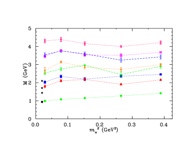
Now we explain how we track the energy eigenstates from one quark mass to the next. Firstly, we label the extracted energy-states at the heaviest quark mass with a chosen set of symbols (most right column in Fig. 2), where each symbol is assigned by the corresponding eigenvectors associated with it. These symbols are carried on to the lightest quark mass by looking at for adjacent quark masses going from the heaviest to the lightest. After the energy eigenstates are labeled at the heaviest quark, we look at the scalar product for the heaviest and the second heaviest quark mass (top left of Table 3). The scalar product shows that in this case all the diagonal elements are larger than the off-diagonal, meaning there is no eigenvector crossing at these two heavier quark masses. A similar scalar product for the second heaviest to the third heaviest mass (top right of Table 3) shows that the fourth and fifth eigenvectors are crossed with the fifth and fourth at the third quark mass, and a similar situation for the sixth and the seventh. To illustrate our analysis in our figures we track the eigenvectors from one quark mass to the next by connecting these similar eigenvectors by lines. In Fig. 2, two lines (eigenvectors) cross at the second and the third quark mass. We then follow the above procedures for the third, fourth and fourth and fifth (the lightest) quark masses.
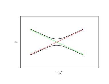
It is well known in quantum mechanics the energies avoid level crossings as illustrated in Fig. 3. However, when two energy levels experience an avoided level crossing, the nature of the two eigenvectors is interchanged, as shown by the dotted lines in Fig. 3. In Fig. 2, the first and second excited energy eigenstates do not experience an avoided level crossing at pion mass of MeV, whereas avoided level crossings are present for the third-fourth and the fifth-sixth excited energy-states. However, note that the avoided level crossings lie within the error bars. Results are presented as a function of quark mass , with where is small. In principle, as noted earlier a similar analysis can be performed for other lattice parameters in addition to the quark mass, such as the lattice spacing , volume , the lattice action etc.
VI Quark-mass Flow of Eigenstates
VI.1 Positive Parity
A key feature of large correlation matrices is the ability to identify and isolate energy eigenstates which are nearly degenerate in energy. However, this approximate degeneracy makes it difficult to trace the flow of states from one quark mass to the next. Thus a clear identification of these near-degenerate states through the features of the eigenvectors isolating the states is necessary in order to trace the propagation of the states from the heavy to the light quark-mass region. At this point it is useful to clarify our use of language. Where we say eigenvector we are referring to the orthogonal eigenvectors, , of our symmetric (or hermitian) correlation matrix . Where we speak of energy eigenvalues and energy eigenstates, we are referring to the eigenvalues and eigenstates of the lattice Hamiltonian, . Our goal in calculations is always to choose the interpolators well so that the few lowest eigenvalues extracted are a good approximation to the few lowest energy eigenvalues of and so that eigenvectors of our correlation matrix capture the dominant characteristics of the corresponding eigenstate of .
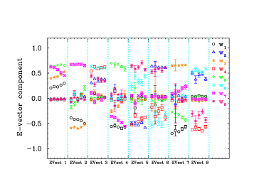
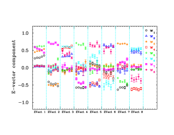
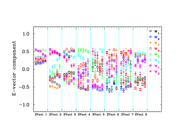
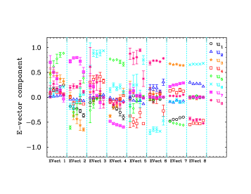
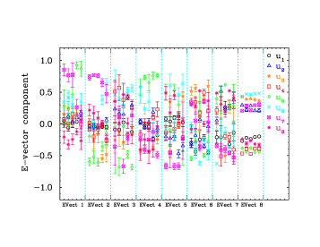
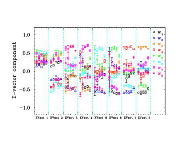
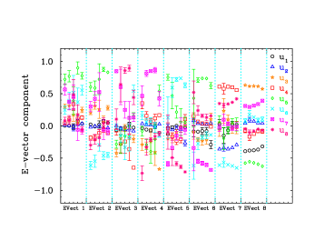
The anticipated and relatively smooth flow of the eigenvectors as a function of the quark mass is presented in Fig. 5. It appears that each eigenvector corresponds to an energy eigenstate of with the eigenvector capturing some of the core properties of the corresponding full energy eigenstate of . While the quark-mass dependent trends can be significant, our approach reliably allows the identification of energy eigenstates at adjacent quark masses.
| 1.00 | -0.09 | 0.00 | 0.00 | 0.01 | 0.00 | 0.01 | 0.00 | 1.00 | -0.08 | 0.01 | -0.01 | 0.01 | 0.01 | 0.00 | 0.00 |
| 0.09 | 0.99 | -0.07 | 0.13 | -0.01 | 0.00 | 0.01 | 0.00 | 0.08 | 0.98 | 0.12 | -0.03 | 0.09 | 0.01 | 0.00 | 0.00 |
| 0.01 | 0.07 | 1.00 | -0.01 | 0.00 | -0.01 | 0.00 | 0.00 | -0.02 | -0.12 | 0.99 | -0.08 | 0.00 | 0.00 | 0.00 | -0.01 |
| -0.01 | -0.13 | 0.02 | 0.98 | -0.09 | 0.02 | 0.07 | 0.00 | -0.01 | -0.09 | -0.01 | 0.03 | 0.99 | -0.10 | 0.00 | 0.00 |
| 0.01 | 0.01 | 0.00 | -0.09 | -0.97 | 0.21 | -0.01 | 0.03 | 0.01 | 0.02 | 0.08 | 0.99 | -0.02 | 0.01 | 0.07 | 0.05 |
| 0.00 | 0.00 | 0.01 | 0.00 | 0.20 | 0.95 | -0.07 | -0.23 | 0.00 | 0.00 | -0.01 | -0.08 | 0.00 | -0.08 | 0.99 | 0.07 |
| -0.01 | 0.00 | 0.00 | -0.07 | 0.01 | 0.07 | 0.99 | -0.01 | 0.01 | 0.02 | 0.00 | 0.01 | -0.10 | -0.99 | -0.08 | 0.03 |
| 0.00 | 0.00 | 0.00 | -0.01 | -0.08 | -0.21 | 0.01 | -0.97 | 0.00 | 0.00 | 0.00 | -0.04 | 0.00 | 0.03 | -0.08 | 1.00 |
| 1.00 | -0.04 | -0.02 | 0.04 | 0.01 | 0.00 | 0.00 | 0.00 | 1.00 | -0.04 | 0.03 | -0.02 | 0.01 | 0.00 | 0.01 | 0.00 |
| 0.03 | 0.98 | -0.21 | 0.04 | -0.01 | 0.00 | -0.03 | 0.00 | 0.03 | 0.97 | 0.25 | 0.06 | -0.02 | -0.01 | -0.01 | -0.01 |
| 0.02 | 0.21 | 0.97 | 0.01 | 0.14 | 0.04 | -0.02 | -0.04 | -0.03 | -0.24 | 0.94 | -0.07 | -0.21 | 0.00 | -0.03 | -0.02 |
| 0.01 | -0.01 | -0.13 | -0.37 | 0.92 | 0.08 | -0.03 | -0.03 | 0.02 | -0.06 | -0.03 | 0.93 | -0.36 | -0.06 | 0.02 | 0.00 |
| -0.04 | -0.04 | -0.05 | 0.93 | 0.36 | 0.02 | 0.00 | -0.01 | -0.01 | -0.05 | 0.20 | 0.35 | 0.89 | -0.03 | -0.21 | -0.01 |
| 0.00 | -0.03 | -0.01 | 0.01 | -0.01 | -0.25 | -0.97 | -0.03 | -0.01 | -0.01 | 0.06 | 0.04 | 0.18 | -0.23 | 0.93 | -0.20 |
| 0.00 | -0.01 | -0.04 | 0.01 | -0.10 | 0.95 | -0.24 | -0.16 | 0.01 | 0.00 | -0.02 | -0.08 | -0.04 | -0.97 | -0.22 | 0.05 |
| 0.00 | -0.01 | -0.02 | 0.00 | -0.02 | -0.15 | 0.07 | -0.99 | 0.01 | 0.00 | -0.04 | -0.02 | -0.04 | 0.00 | -0.20 | -0.98 |
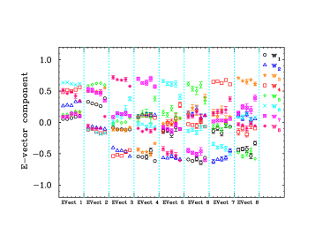
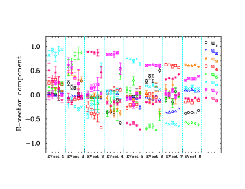
As the and spin-flavor interpolators are very similar for the channel, the overall flow of the eigenvectors obtained from the and correlation matrices are very similar in Fig. 5. Also, the overall strength of the eigenvector components creating and annihilating energy-states in the QCD vacuum remains approximately the same for the and cases (Fig. 6), which implies that the eigenstate-energies isolated by the and analysis are the same. As the first excited state is purely -spin-flavour dominated, this state is revealed in all the three different correlation matrix analyses.
There are a few general trends apparent in Figs. 6(a) and 6(b) which are worthy of note. Focusing on 6(a) for specific reference, we see that there is often competition between different smearing levels in creating the states. A good example is in state two, where the 200 sweep interpolator is complemented by the 35 sweep interpolator at heavy quark masses, but the 35 sweep interpolator strength is phased out as one approaches light quark masses with strength transitioning to the 100 sweep interpolator. Even in the ground state one can see the importance of the 200 sweep interpolator increasing as one approaches the lighter masses. This effect is even stronger in Fig. 6(b) for the analysis where the 100 sweep operator is phased out in favour of the 200 sweep .
One can also observe the superposition of Gaussian smearings of different sizes being superimposed with relative minus signs in a manner that will create nodes in the radial wave function of the interpolator of Eq. (20). Focusing again on Fig. 6(a) to provide a specific example, consider state 2. Here the widest Gaussian of 200 sweeps is complemented by a smaller Gaussian with the opposite sign. Moreover, as the quark masses become light, the smaller Gaussian grows in size. The result is that the radial node position of the wave function increases in distance as the quarks become lighter.
Similarly, state 4 involves the superposition of three Gaussian smearings with alternating signs. Here the 200 sweep interpolator is complemented with the 100 sweep interpolator with opposite sign which is complemented further by the 35 sweep operator, again with the opposite sign. Such a linear combination can create two nodes in the radial wave function.
Finally, state 7 combines the 200, 100, 35 and 16 sweep interpolators with alternating signs such that a state with three nodes could be accessed.
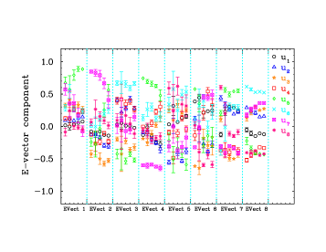
Turning our attention to the analysis, we see the flow of eigenvector components is not as smooth. Figures 5(c) and 6(c) present the flow of the eigenvectors for this analysis. A careful comparison of the eigenstate spectrum with that from the analysis at each quark mass and consideration of the eigenvector flow of the states reveals that the states dominated by in the analysis are reproduced in the analysis. However, the remaining four states display a flow different from those revealed in the analysis. Thus, a superposition of the and analysis provides unique energy states.
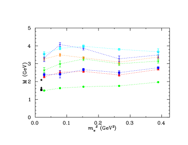
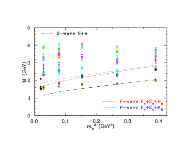
In Fig. 7, a superposition of the two analysis of and is presented. Scattering -wave and -wave energy levels are also shown.
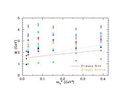
For the two large quark masses, as seen in Fig. 7, the extracted lattice results sit close to the scattering two particle -wave threshold () with back-to-back momenta, and -wave threshold (), whereas the masses for the lighter three quarks sit much higher. There is no evidence of these scattering states at light quark masses. Our conclusion is that our 3-quark operators have very little coupling to the multi-hadron states relative to the states we do observe at the light quark masses.
It is noted that the couplings to the multi-particle meson-baryon states are suppressed by relative to states dominated by a single-particle state. Due to the large volume of our lattice, it is likely that multi-particle states will be suppressed and missed in our spectrum, particularly at lighter quark masses where the quark-mass effect also acts to suppress the spectral strength. Further analysis of finite volume effects Young et al. (2002) on the spectrum is highly desirable. Future calculations should also investigate the use of five-quark operators to ensure better overlap with the multi-particle states and to better resolve and probe the excited state spectrum Morningstar et al. (2011); Lang and Verduci (2012); Morningstar et al. (2013).
VI.2 Negative Parity
Now we can repeat our analysis for the identification of the states. In Table 4, the scalar product for all the quark masses is presented.
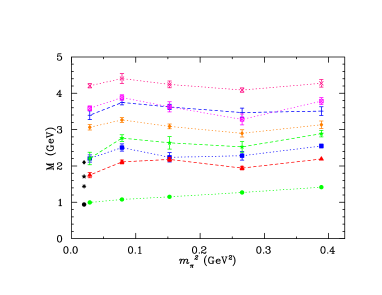
In Figs. 8 and 9, the spectrum from the analysis involving and is presented, respectively. While the analysis is able to extract a low-lying energy state, it misses the near-degenerate second energy state in this channel. This second energy-state is revealed in the spin-flavor combination presenting two nearly-degenerate low-lying states, which is in accord with the quark model based on spin-flavor symmetry. Recall that three spin- quarks may provide a total spin of or , the state can couple two different ways to provide a state, hence providing two orthogonal spin- states in the , 70 plet representation of . Both of these states have a width of 150 MeV.
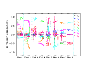
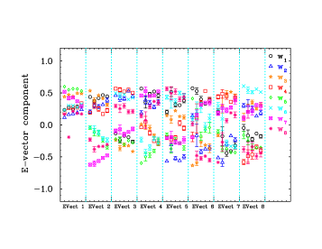
As in Fig. 5, the eigenvector components for different quark masses are presented in Figs. 10 and 11 for the channel. It is interesting to note that the scalar-diquark interpolator dominates the lowest two states (Fig. 11) when available. The interpolator makes an important contribution in creating the second energy state in this channel.
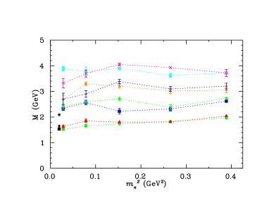
In Fig. 12, a superposition of the two analysis of and is presented. Scattering -wave and -wave states are also shown. The results for the lowest energy-state at the two heavier pion masses sit close to the scattering s-wave () threshold indicating that these results may be scattering states at these pion masses. However, they disappear from our spectrum at the light pion masses. A similar situation also prevails the second energy-state, where the state sits close to the -wave and scattering threshold with back-to-back momenta of one lattice unit, . Again the use of 5- or 7- etc. quark meson-baryon operators will be required to explore these scattering states Morningstar et al. (2011); Lang and Verduci (2012); Morningstar et al. (2013).
| -0.03 | 0.99 | -0.08 | -0.04 | 0.05 | -0.01 | 0.00 | 0.01 | -0.22 | 0.97 | 0.04 | -0.10 | -0.01 | 0.04 | 0.01 | -0.02 |
| 1.00 | 0.02 | 0.01 | -0.08 | -0.02 | -0.01 | 0.00 | 0.01 | 0.97 | 0.22 | -0.07 | -0.07 | 0.01 | 0.02 | -0.02 | -0.01 |
| 0.00 | 0.07 | 0.97 | 0.05 | 0.22 | -0.03 | -0.04 | 0.00 | 0.07 | -0.03 | 0.99 | -0.04 | 0.07 | 0.00 | -0.02 | -0.01 |
| 0.07 | 0.03 | -0.07 | 0.96 | 0.01 | -0.27 | 0.00 | -0.02 | 0.05 | 0.11 | 0.04 | 0.99 | -0.01 | 0.05 | 0.01 | -0.04 |
| -0.02 | 0.06 | 0.20 | 0.02 | -0.95 | -0.01 | -0.23 | -0.01 | -0.01 | 0.02 | -0.07 | 0.02 | 0.99 | -0.09 | 0.04 | 0.03 |
| 0.03 | 0.02 | 0.01 | 0.26 | 0.00 | 0.94 | -0.01 | -0.21 | 0.02 | 0.04 | 0.01 | 0.04 | -0.09 | -0.99 | -0.02 | -0.02 |
| -0.01 | 0.02 | 0.08 | 0.01 | -0.22 | 0.01 | 0.97 | 0.01 | 0.02 | -0.01 | 0.01 | -0.01 | -0.04 | -0.01 | 0.99 | -0.13 |
| 0.00 | 0.00 | 0.00 | 0.08 | 0.00 | 0.20 | -0.02 | 0.98 | 0.01 | 0.02 | 0.02 | 0.03 | -0.03 | -0.02 | 0.12 | 0.99 |
| 0.91 | 0.40 | 0.02 | 0.02 | 0.01 | -0.05 | 0.00 | 0.00 | 0.98 | 0.17 | -0.06 | -0.01 | 0.01 | 0.01 | 0.00 | 0.00 |
| 0.40 | -0.91 | 0.00 | 0.01 | -0.02 | 0.01 | -0.01 | 0.00 | -0.17 | 0.99 | -0.01 | -0.03 | 0.01 | 0.01 | -0.01 | 0.00 |
| -0.01 | -0.01 | 0.96 | -0.27 | 0.01 | -0.01 | 0.00 | 0.02 | 0.05 | 0.03 | 0.77 | 0.64 | -0.01 | 0.00 | 0.00 | 0.02 |
| -0.03 | 0.00 | 0.27 | 0.96 | 0.01 | 0.01 | 0.02 | 0.00 | 0.04 | -0.01 | 0.64 | -0.77 | -0.04 | 0.00 | 0.01 | 0.00 |
| 0.04 | 0.03 | 0.01 | -0.01 | -0.22 | 0.97 | 0.02 | 0.01 | 0.00 | 0.00 | 0.02 | -0.01 | 0.66 | -0.75 | -0.04 | -0.01 |
| 0.01 | -0.01 | -0.01 | -0.01 | 0.98 | 0.22 | 0.04 | 0.00 | -0.01 | -0.01 | 0.03 | -0.02 | 0.75 | 0.66 | -0.04 | -0.02 |
| 0.00 | 0.00 | -0.02 | 0.01 | 0.01 | -0.01 | -0.12 | 0.99 | 0.00 | 0.01 | 0.00 | 0.01 | 0.05 | -0.01 | 0.96 | -0.26 |
| 0.01 | -0.01 | 0.00 | -0.02 | -0.04 | -0.03 | 0.99 | 0.12 | 0.00 | 0.00 | -0.01 | -0.01 | 0.04 | 0.01 | 0.26 | 0.96 |
VII Conclusions
In this paper, a comprehensive analysis for the nucleon spectrum with , , is presented using the correlation matrix approach. In particular, a method for energy-eigenstate identification and flow is presented and demonstrated for the positive and negative parity channel. Details of the method developed for an identification and the propagation of the energy-states from heavy to light quark mass region are provided. In particular, the new technique is useful in identifying the flow of the near-degenerate energy eigenstates from one quark mass to the next. The eigenvectors obtained from the eigenvalue equations for several correlation matrices are utilized in tracking the eigen-energy states.
In presenting the results, both non-symmetric left and right eigenvalue equations and a symmetric eigenvalue equation are considered. While the masses are the same in the two different approaches, the eigenvectors obtained from the symmetric matrix are orthogonal. Thus the generalized measure is used to track the flow of eigenvectors with quark mass. The scalar product of the eigenvectors shows its robustness in tracking the flow of the energy eigenstates even when the energies are nearly degenerate.
The coefficients of the interpolators creating and annihilating a state in the QCD vacuum are also presented. The flow of the eigenvectors reveals a smooth pattern and presents important insights into baryon structure and its evolution with quark mass.
Another interesting result of this paper is that, the correlation matrix method can be used to track the energy-states that are involved in an avoided level crossing. It is noted that the avoided level crossings lie within the error bars, but the demonstration of the robustness of the approach remains.
Future steps include the introduction of five-quark meson-baryon operators in the correlation matrices, to ensure the clear isolation of states and ultimately extract the resonance parameters from the first principles of QCD.
Acknowledgements.
We thank PACS-CS Collaboration for making these flavor configurations available. This research was undertaken on the NCI National Facility in Canberra, Australia, which is supported by the Australian Commonwealth Government. We also acknowledge eResearch SA for generous grants of supercomputing time which have enabled this project. This research is supported by the Australian Research Council.*
Appendix A Pedagogical Discussion of the Correlation Matrix
A.1 For
Let us consider an dimensional Hilbert space with a hamiltonian, , and let , , , be linearly independent states. Similarly, let , , , be a complete orthonormal basis of energy eigenstates, then the state can be written as
| (41) |
where, , which is analogous to Eq. (7). In matrix form Eq. (41) can be written as
| (48) |
Since is linearly independent, then must be non-singular and so there must exist such that
| (55) |
Similarly, can be expressed as .
Let us now define for linearly independent field operators , where the dagger denotes the adjoint. Then we may write
or,
| (59) | ||||
| (60) |
where, is obviously diagonal. The Eq. (60) is analogous to Eq. (19). From this point on for notational convenience we will no longer use square brackets to denote matrices. We see that, for all . From Eq. (60), we can also write
| (61) |
where, and . Similarly, we can write
| (62) |
Let us consider the polar decomposition of as
, where is unitary
Similarly, . Then, Eq. (62) can be written as
| (63) |
or equivalently
| (64) |
where we are using the notation
| (68) |
Denoting the normalized eigenvectors of as for , then consists of columns . Hence we see that
| (69) |
Multiplying Eq. (69) by from left and defining
| (70) |
gives
| (71) |
which is analogous to Eq. (26).
A.2 For
Let , , , be linearly independent interpolating field operators with . Then we may consider these ’s as a subset of a complete set of interpolating operators. Then as before, we can define as an correlation matrix, then can be written as the upper left block of such that
| (74) |
where the off-diagonal rectangular matrix has elements for and . Clearly mixes the upper and lower diagonal blocks.
In terms of the full correlation matrix we define as before and it has the form
| (77) |
which is of course diagonalized by the full unitary matrix as shown in Eq. (64).
Let us now temporarily assume that the off-diagonal elements of are zero, then
| (80) |
and then it follows that the time independent unitary matrix can be written as
| (83) |
This will occur if and only if we have chosen our interpolating fields such that they span exactly the same subspace as of the exact energy eigenstates.
But we will certainly never exactly achieve this and so mixing will occur through . In this case will not have this convenient block diagonal form. Let diagonalize , i.e. is an unitary matrix defined at this particular . Then if we see that and in general will not be independent of . Note that linearly independent interpolating field operators will operate on the vacuum and give rise to linearly independent states. The more closely these linearly independent states come to spanning the same subspace as exact energy eigenstates, then the smaller will be and the more block diagonal will be and . We can only ensure that commutes with itself at all if is block diagonal, i.e., if so that and is therefore time independent. Then the smaller will be the off-diagonal elements and the smaller will be the mixing and the excited state contamination.
In practice , since on a lattice the dimensionality of Hilbert space is in the many millions. We would like to choose the interpolating fields such that they span an -dimensional subspace that has the greatest overlap possible with the subspace spanned by the lowest energy eigenstates . With the lowest energy eigenstates our numerical errors will be minimized, since by working at large Euclidean times we minimize the influence of the higher excited state contamination and so optimize our extraction of the lowest energy eigenstates.
Since the interpolating fields produced states that were not normalized in any way, it is numerically convenient to redefine
where there is no sum over . Therefore, we attempt to put the strengths of our interpolating fields at a comparable level by defining
to ensure that the matrix elements of are all to maximize numerical significance of all “” combinations. This is completely legitimate as it is simply a change to the normalization chosen for our interpolating fields, which we are free to do. The matrix is hermitian except for the effects of finite ensemble and round-off errors. Let us define
| (84) |
as an improved unbiased estimator of the ensemble average for . Then is exactly hermitian. Therefore, as before, we may diagonalize
| (85) |
which is also hermitian, as and are obviously hermitian. The eigenvectors () obtained from diagonalizing the above matrix are therefore orthonormal. It is noted that using the trick Melnitchouk et al. (2003), where these ’s are links here, the hermitian correlation matrix is real symmetric and so the eigenvalues remain real and the eigenvectors orthogonal. Again, it is important to note that the more poorly we choose our interpolating fields then the bigger will be the off-diagonal elements of . Hence the more time-dependent will be the and the less reliable our extracted energies and eigenvectors.
Now we can consider as a function of quark mass, , to identify how a given state evolves with . If with small, we expect if and if .
References
- Durr et al. (2008) S. Durr et al., Science 322, 1224 (2008), arXiv:0906.3599 [hep-lat] .
- Roper (1964) L. D. Roper, Phys. Rev. Lett. 12, 340 (1964).
- Isgur and Karl (1977) N. Isgur and G. Karl, Phys. Lett. B72, 109 (1977).
- Isgur and Karl (1979) N. Isgur and G. Karl, Phys. Rev. D19, 2653 (1979).
- Li et al. (1992) Z.-p. Li, V. Burkert, and Z.-j. Li, Phys. Rev. D46, 70 (1992).
- Carlson and Mukhopadhyay (1991) C. E. Carlson and N. C. Mukhopadhyay, Phys. Rev. Lett. 67, 3745 (1991).
- Guichon (1985) P. A. M. Guichon, Phys. Lett. B164, 361 (1985).
- Krehl et al. (2000) O. Krehl, C. Hanhart, S. Krewald, and J. Speth, Phys. Rev. C62, 025207 (2000), arXiv:nucl-th/9911080 .
- Allton et al. (1993) C. R. Allton et al. (UKQCD), Phys. Rev. D47, 5128 (1993), hep-lat/9303009 .
- Lee and Leinweber (1999) F. X. Lee and D. B. Leinweber, Nucl. Phys. Proc. Suppl. 73, 258 (1999), arXiv:hep-lat/9809095 .
- Gockeler et al. (2002) M. Gockeler et al. (QCDSF), Phys. Lett. B532, 63 (2002), arXiv:hep-lat/0106022 .
- Sasaki et al. (2002) S. Sasaki, T. Blum, and S. Ohta, Phys. Rev. D65, 074503 (2002), hep-lat/0102010 .
- Melnitchouk et al. (2003) W. Melnitchouk et al., Phys. Rev. D67, 114506 (2003), hep-lat/0202022 .
- Edwards et al. (2003) R. G. Edwards, U. M. Heller, and D. G. Richards (LHP), Nucl. Phys. Proc. Suppl. 119, 305 (2003), arXiv:hep-lat/0303004 .
- Lee et al. (2003) F. X. Lee et al., Nucl. Phys. Proc. Suppl. 119, 296 (2003), hep-lat/0208070 .
- Brommel et al. (2004) D. Brommel et al. (Bern-Graz-Regensburg), Phys. Rev. D69, 094513 (2004), hep-ph/0307073 .
- Mathur et al. (2005) N. Mathur et al., Phys. Lett. B605, 137 (2005), hep-ph/0306199 .
- Sasaki (2003) S. Sasaki, Prog. Theor. Phys. Suppl. 151, 143 (2003), arXiv:nucl-th/0305014 .
- Burch et al. (2004) T. Burch et al. (Bern-Graz-Regensburg), Phys. Rev. D70, 054502 (2004), hep-lat/0405006 .
- Basak et al. (2007) S. Basak et al., Phys. Rev. D76, 074504 (2007), arXiv:0709.0008 [hep-lat] .
- Mahbub et al. (2009a) M. S. Mahbub et al., Phys. Rev. D80, 054507 (2009a), arXiv:0905.3616 [hep-lat] .
- Mahbub et al. (2009b) M. S. Mahbub et al., Phys. Lett. B679, 418 (2009b), arXiv:0906.5433 [hep-lat] .
- Fleming et al. (2009) G. T. Fleming, S. D. Cohen, H.-W. Lin, and V. Pereyra, Phys. Rev. D80, 074506 (2009), arXiv:0903.2314 [hep-lat] .
- Mahbub et al. (2010a) M. S. Mahbub, A. O. Cais, W. Kamleh, D. B. Leinweber, and A. G. Williams, Phys. Rev. D82, 094504 (2010a), arXiv:1004.5455 [hep-lat] .
- Mahbub et al. (2010b) M. S. Mahbub, W. Kamleh, D. B. Leinweber, A. O. Cais, and A. G. Williams, Phys. Lett. B693, 351 (2010b), arXiv:1007.4871 [hep-lat] .
- Bulava et al. (2009) J. M. Bulava et al., Phys. Rev. D79, 034505 (2009), arXiv:0901.0027 [hep-lat] .
- Engel et al. (2010) G. P. Engel, C. B. Lang, M. Limmer, D. Mohler, and A. Schafer (BGR [Bern-Graz-Regensburg]), Phys. Rev. D82, 034505 (2010), arXiv:1005.1748 [hep-lat] .
- Edwards et al. (2011) R. G. Edwards, J. J. Dudek, D. G. Richards, and S. J. Wallace, Phys. Rev. D84, 074508 (2011), arXiv:1104.5152 [hep-ph] .
- Mahbub et al. (2012) M. S. Mahbub, W. Kamleh, D. B. Leinweber, P. J. Moran, and A. G. Williams (CSSM Lattice), Phys. Lett. B707, 389 (2012), arXiv:1011.5724 [hep-lat] .
- Lin and Cohen (2011) H.-W. Lin and S. D. Cohen, (2011), arXiv:1108.2528 [hep-lat] .
- Michael (1985) C. Michael, Nucl. Phys. B259, 58 (1985).
- Luscher and Wolff (1990) M. Luscher and U. Wolff, Nucl. Phys. B339, 222 (1990).
- Lin et al. (2009) H.-W. Lin et al. (Hadron Spectrum), Phys. Rev. D79, 034502 (2009), arXiv:0810.3588 [hep-lat] .
- Bulava et al. (2010) J. Bulava et al., Phys. Rev. D82, 014507 (2010), arXiv:1004.5072 [hep-lat] .
- Morningstar et al. (2011) C. Morningstar et al., Phys. Rev. D83, 114505 (2011), arXiv:1104.3870 [hep-lat] .
- Bulava (2011) J. Bulava, (2011), arXiv:1112.0212 [hep-lat] .
- Menadue et al. (2011) B. J. Menadue, W. Kamleh, D. B. Leinweber, and M. S. Mahbub, (2011), arXiv:1109.6716 [hep-lat] .
- Edwards et al. (2012) R. G. Edwards, N. Mathur, D. G. Richards, and S. J. Wallace, (2012), arXiv:1212.5236 [hep-ph] .
- Engel et al. (2013) G. P. Engel, C. Lang, D. Mohler, and A. Schaefer, (2013), arXiv:1301.4318 [hep-lat] .
- Aoki et al. (2009) S. Aoki et al. (PACS-CS), Phys. Rev. D 79, 034503 (2009), arXiv:0807.1661 [hep-lat] .
- Mahbub et al. (2013) M. S. Mahbub, W. Kamleh, D. B. Leinweber, P. J. Moran, and A. G. Williams (CSSM Lattice Collaboration), Phys.Rev. D87, 011501 (2013), arXiv:1209.0240 [hep-lat] .
- Lang and Verduci (2012) C. Lang and V. Verduci, (2012), arXiv:1212.5055 [hep-lat] .
- Morningstar et al. (2013) C. Morningstar, J. Bulava, B. Fahy, J. Foley, Y. Jhang, et al., (2013), arXiv:1303.6816 [hep-lat] .
- Gusken (1990) S. Gusken, Nucl. Phys. Proc. Suppl. 17, 361 (1990).
- Blossier et al. (2009) B. Blossier, M. Della Morte, G. von Hippel, T. Mendes, and R. Sommer, JHEP 04, 094 (2009), arXiv:0902.1265 [hep-lat] .
- Beckett et al. (2011) M. G. Beckett et al., Comput. Phys. Commun. 182, 1208 (2011), arXiv:0910.1692 [hep-lat] .
- Iwasaki (1983) Y. Iwasaki, (1983), uTHEP-118.
- Leinweber et al. (1991) D. B. Leinweber, R. M. Woloshyn, and T. Draper, Phys. Rev. D43, 1659 (1991).
- Leinweber (1995) D. B. Leinweber, Phys. Rev. D51, 6383 (1995), nucl-th/9406001 .
- Zanotti et al. (2003) J. M. Zanotti et al. (CSSM Lattice), Phys. Rev. D68, 054506 (2003), hep-lat/0304001 .
- Young et al. (2002) R. D. Young, D. B. Leinweber, A. W. Thomas, and S. V. Wright, Phys. Rev. D66, 094507 (2002), arXiv:hep-lat/0205017 .