Also at ]Argonne National Laboratory, USA
Also at ] University of Huddersfield, West Yorkshire, United Kingdom and CERN, Genf
A Parallel General Purpose Multi-Objective Optimization Framework, with Application To Electron Beam Dynamics
Abstract
Particle accelerators are invaluable tools for research in the basic and applied sciences, such as materials science, chemistry, the biosciences, particle physics, nuclear physics and medicine. The design, commissioning, and operation of accelerator facilities is a non-trivial task, due to the large number of control parameters and the complex interplay of several conflicting design goals. The Argonne Wakefield Accelerator facility has some unique challenges resulting from its purpose to carry out advanced accelerator R&D. Individual experiments often have challenging beam requirements, and the physical configuration of the beamlines is often changed to accommodate the variety of supported experiments. The need for rapid deployment of different operational settings further complicates the optimization work that must be done for multiple constraints and challenging operational regimes. One example of this is an independently staged two-beam acceleration experiment which requires the construction of an additional beamline (this is now in progress). The high charge drive beam, well into the space charge regime, must be threaded through small aperture (17.6 mm) decelerating structures. In addition, the bunch length must be sufficiently short to maximize power generation in the decelerator. We propose to tackle this problem by means of multi-objective optimization algorithms which also facilitate a parallel deployment. In order to compute solutions in a meaningful time frame, a fast and scalable software framework is required. In this paper, we present a general-purpose framework for simulation-based multi-objective optimization methods that allows the automatic investigation of optimal sets of machine parameters. Using evolutionary algorithms as the optimizer and OPAL as the forward solver, validation experiments and results of multi-objective optimization problems in the domain of beam dynamics are presented. Optimized solutions for the new high charge drive beamline found by the framework were used to finish the design of a two beam acceleration experiment. The selected solution along with the associated beam parameters is presented.
I INTRODUCTION
Particle accelerators play a significant role in many aspects of science and technology. Fields, such as material science, chemistry, the biosciences, particle physics, nuclear physics and medicine depend on reliable and effective particle accelerators, both as research and practical tools. Achieving the required performance in the design, commissioning, and operation of accelerator facilities is a complex and versatile problem. Despite the success of on-line models in some facilities Huang (2018), and various model dependent and model independent tuning and optimization techniques, empirical tuning by operators is a common method used at many research facilities. When the beam dynamics is nonlinear, as is the case with space charge, simple and fast models are applicable only in a very restricted manner. This further complicates any mult-objective optimization by complicating the model. In order to be able to reliably identify optimal configurations of accelerators, we solve large multi-objective design optimization problems to automate the investigation for an optimal set of tuning parameters. This approach has been used in the past with much success Hofler et al. (2013); Bazarov and Sinclair (2005); Yang et al. (2009); Terzic et al. (2014); Gulliford et al. (2016, 2017); Kranjčević et al. (2019). The difference here being the implementation and application to a problem at the Argonne Wakefield Accelerator Facility (AWA).
A hallmark of the AWA facility is the flexibility to swap physical components in the beamlines, which enables different, often novel, accelerator research experiments to take place. Not only do the physical machine components change, the beam characteristics also vary considerably to meet different needs. The facility operates at both low and high charge (up to 100 nC), and at high charge strong nonlinearities require a full 3D space charge approach in simulations. Finding optics solutions in this regime, especially when there are additional constraints such as the small aperture two-beam accelerating structures, is challenging even without the quick turnaround of the beamline configurations. Therefore, it has been an important research objective to develop a precise, e.g. 3D model embedded into a multi-objective optimization framework that may be used as a flexible platform for optimization of changing machine configurations operated at different charge levels. While other codes, such as GPT Physics (2018) and ELEGANT Borland (2018), also have integrated genetic optimization algorithms; the OPAL Adelmann et al. (2018) framework differentiates itself by being open source (i.e. free to use), massively parallel, and fully 3D.
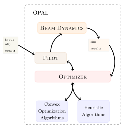
A modular multi-objective software framework was developed (see Fig. 1) where the core functionality of the optimizer is decoupled from the “beam dynamics” but fully integrated in the OPAL framework. To that end, we use a master/slave mechanism where a master process governs a set of slave processes given some computational tasks (beam dynamics simulation) to complete. This separation allows easy interchange of optimization algorithms, forward solvers and optimization problems. A “pilot” coordinates all efforts between the optimization algorithm and the beam dynamics task. In the following sections, we will also use the notion of “forward solver” to indicate the beam dynamics task. This forms a robust and general framework for massively parallel multi-objective optimization. Currently the framework offers one concrete optimization algorithm, an evolutionary algorithm employing a NSGA-II selector Bleuler et al. (2003). Normally, simulation based approaches are plagued by the trade off between level of detail and time to solution. This problem is addressed later in Section (V.2.1) by using forward solvers with different time and resolution complexity.
The framework discussed here, incorporates the following three contributions:
-
1.
Implementation of a scalable optimization algorithm capable of approximating Pareto fronts in high dimensional spaces,
-
2.
design and implementation of a modular framework that is simple to use and deploy on large scale computational resources, and
-
3.
demonstration of the usefulness of the proposed framework on a real world application in the domain of particle accelerators. This is done with the optimization problem set as the high charge photoinjector at the AWA.
The next section introduces the notation of multi-objective optimization theory and describes the first implemented optimizer. In Section III, the implementation of the framework is discussed. We introduce the employed forward-solver in Section IV. A validation and a proof of concept application in the beam dynamics problems mentioned above is discussed in Section V.
II MULTI-OBJECTIVE OPTIMIZATION
Optimization problems deal with finding one or more feasible solutions corresponding to extreme values of objectives. If more than one objective is present in the optimization problem this is called a multi-objective optimization problem (MOOP). A MOOP is defined as
| min | (1) | |||||
| s.t. | (2) | |||||
| (3) |
where denotes the objectives (1), the constraints (2), and the design variables (3). Often, conflicting objectives are encountered, and this complicates the concept of optimality. Pareto optimality is often used in such situations. The set of Pareto optimal points forms the Pareto front or surface. All points on this surface are considered to be Pareto optimal. Sampling Pareto fronts is far from trivial. A number of approaches have been proposed, e.g. evolutionary algorithms Deb (2009), simulated annealing Kirkpatrick et al. (1983), swarm methods Kennedy and Eberhart (1995), and many more Dorigo et al. (1996); De Castro and Timmis (2002); Karaboga (2005); Shah-Hosseini (2009). In the next section, we briefly introduce the theory of evolutionary algorithms used in the present work.
II.1 Evolutionary Algorithms
Evolutionary algorithms are loosely based on nature’s evolutionary principles to guide a population of individuals towards an improved solution by honoring the “survival of the fittest” principle. This “simulated” evolutionary process preserves entropy (or diversity in biological terms) by applying genetic operators, such as mutation and crossover, to remix the fittest individuals in a population. Maintaining diversity is a crucial feature for the success of all evolutionary algorithms.
In general, a generic evolutionary algorithm consists of the following components:
-
•
Genes: traits defining an individual,
-
•
Fitness: a mapping from genes to a fitness value for each individual,
-
•
Selector: selecting the fittest individuals of a population based on some sort of ordering,
-
•
Variator: recombination (mutations and crossover) operators for offspring generation.
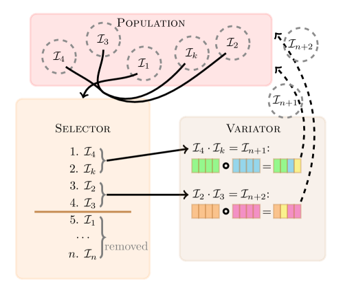
Applied to multi-objective optimization problems, genes correspond to design variables. The fitness of an individual is loosely related to the value of the objective functions for the corresponding genes. Figure 2 schematically depicts the connection of the components introduced above. The process starts with an initially random population of individuals, each individual with a unique set of genes and corresponding fitness, representing one location in the search space. In the next step, the population is processed by the selector determining the fittest individuals according to their fitness values. While the fittest individuals are passed to the variator, the remaining individuals are eliminated from the population. The Variator mates and recombines the fittest individuals to generate new offspring. After evaluating the fitness of all the freshly born individuals a generation cycle has completed and the process can start anew.
Since there already exist plenty of implementations of evolutionary algorithms, it was decided to incorporate the PISA library Bleuler et al. (2003) into our framework. One of the advantages of PISA is that it separates variator from selector, rendering the library expandable and configurable. Implementing a variator was enough to use PISA in our framework and retain access to all available PISA selectors. As shown in Fig. 2, the selector is in charge of ordering a set of -dimensional vectors and selecting the fittest individuals currently in the population. The performance of a selector depends on the number of objectives and the surface of the search space. So far, the NSGA-II selector Deb et al. (2002) has been used and exhibits satisfactory convergence performance.
The task of the variator is to generate offspring and ensure diversity in the population. The variator can start generating offspring once the fitness of every individual of the population has been evaluated. This explicit synchronization point defines an obvious bottleneck for parallel implementations of evolutionary algorithms. In the worst case, some MPI processes are taking a long time to compute the fitness of the last individual in the pool of individuals to evaluate. During this time all other resources are idle and wait for the result of this one individual in order to continue to generate and evaluate offspring. To counteract this effect, the selector is already called when two individuals have finished evaluating their fitness, lifting the boundaries between generations and evaluating the performance of individuals. New offspring will be generated and MPI processes can immediately return to work on the next fitness evaluation. By calling the selector more frequently (already after two offspring individuals have been evaluated) results in better populations since bad solutions are rejected earlier. On the other hand, calling the selector more often is computationally more expensive. Note this capability is also present in GPT’s Physics (2018) optimization system.
The variator implementation uses the master/slave architecture, presented in the next section, to run as many function evaluations as possible in parallel. Additionally, various crossover and mutation policies are available for tuning the algorithm to the optimization problem.
III THE FRAMEWORK
Simulation based multi-objective optimization problems are omnipresent in research and industry. These simulation and optimization problems are in general very big and computationally demanding. This motivated us to design a massively parallel general purpose framework. The key traits of such a design can be summarized as:
-
•
support any multi-objective optimization method,
-
•
support any function evaluator: simulation code or measurements,
-
•
offer a general description/specification of objectives, constraints and design variables,
-
•
run efficiently in parallel on current large-scale high-end clusters and supercomputers.
III.1 Related Work
Several similar frameworks, e.g. Filipič and Depolli (2009); León et al. (2009); Liefooghe et al. (2007); Durillo et al. (2006), have been proposed. Commonly these frameworks are tightly coupled to an optimization algorithm, e.g. only providing evolutionary algorithms as optimizers. Users can specify optimization problems, but cannot change the optimization algorithm. Our framework follows a more general approach, providing a user-friendly way to introduce new or choose from existing built-in multi-objective optimization algorithms. Tailoring the optimization algorithm to the optimization problem at hand is an important feature due to the many different characteristics of optimization problems that should be handled by such a general framework. As an example, it is shown how Pisa Bleuler et al. (2003), an existing evolutionary algorithm library, was integrated with ease. Similarly, other multi-objective algorithms could be incorporated and used to solve optimization problems.
The framework presented in León et al. (2009) resembles our implementation the most, aside from their tight coupling with an evolutionary algorithm optimization strategy. The authors propose a plug-in based framework employing an island parallelization model, where multiple populations are evaluated concurrently and independently up to a point where some number of individuals of the population are exchanged. This is especially useful to prevent the search algorithm to get stuck in a local minimum. A set of default plug-ins for genetic operators, selectors and other components of the algorithms are provided by their framework. User-based plug-ins can be incorporated into the framework by implementing a simple set of functions.
Additionally, as with simulation based multi-objective optimization, we can exploit the fact that both the optimizer and simulation part of the process use a certain amount of resources. The ratio of work between optimizer and simulation costs can be reflected in the ratio of number of processors assigned to each task. This not only provides users with great flexibility in using any simulation or optimizer, but renders influencing the role assignment easy as well.
III.2 Components
The basic assumption in simulation-based optimization is that a call to an expensive simulation software component present in the constraints or objectives is needed. The framework is divided in three exchangeable components, as shown in Fig. 3, to encapsulate the major behavioral patterns of the framework.
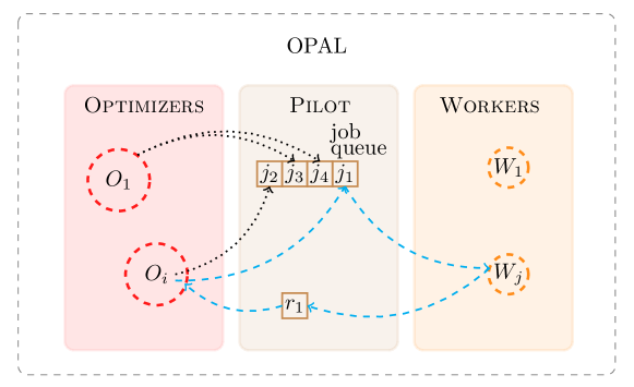
The Pilot component acts as a bridge between the optimizer and forward solvers, providing the necessary functionality to handle passing requests and results between the Optimizer and the Simulation modules. The framework was implemented in C++, utilizing features like template parameters to specify the composition of the framework. “Default” implementations are provided that can be controlled via command line options. Due to its modular design, all components can be completely customized.
Every available MPI process will take up one of the three available roles (see Fig. 1): one process acts as Pilot, the remaining processes are divided amongst Worker and Optimizer roles. Both, the Worker and the Optimizer can consist of multiple MPI processes to exploit parallelism. As shown in Fig. 3, the Pilot is used to coordinate all “information requests” between the Optimizer and the Worker. An information request is a job that consists of a set of design variables (e.g. the genes of an individual) and a type of information it requests (e.g. function evaluation or derivative). The Pilot keeps checking for idle Worker and assigns jobs in the queue to any free Worker. Once the Worker has computed and evaluated the request its results are returned to the Optimizer that originally requested the information.
After a process gets appointed a role, it starts a polling loop to asynchronously check for appropriate incoming requests. To that end a Poller interface helper class has been introduced. The Poller interface consists of an infinite loop that checks periodically for new MPI messages. Upon reception a new message is immediately forwarded to the appropriate handler: the onMessage() method. The method is called with the MPI_Status of the received message and a size_t value specifying different values depending on the value of the MPI_Tag. The Poller interface allows the implementation of special methods (denoted hooks) determining the behavior of the polling process, e.g. for actions that need to be taken after a message has been handled. Every Poller terminates the loop upon receiving a special MPI tag.
III.3 Implementing an Optimizer
All Optimizer implementations have to respect the API shown in Listing 2.
Code Listing 2: Optimizer API
All processors running an Optimizer component call the initialize entry point after role assignment in the Pilot. The implementation of initialize must set up and start the poller and the optimization code. Since an optimizer derives from the Poller interface, predefined hooks can be used to determine the polling procedure. Hooks can be implemented as empty methods, but the onMessage implementation should reflect the optimization part of the protocol for handling events from the Pilot. A special set of communicator groups serves as communication channels to the Pilot, its job queue, and processes supporting the Optimizer component.
III.4 Implementing a Forward Solver
In most cases, forward solver implementations are simple wrappers to run an existing “external” simulation code using a set of design variables as input. In the case of the OPAL integration, the main function is playing the role of the “forward solver”. To underline the general nature of our approach, in a similar project, the described methods are used for cavity shape optimisation based on Arbenz and Chinellato (2008). As for the Optimizer component there exists a base class, labeled Simulation as common basis for all Simulation implementations. In addition, this component also inherits from the Worker class, already implementing the polling protocol for default worker types. As shown in the API in Listing 3, the Worker class expects an implementation to provide implementations for those three methods.
Code Listing 2: Simulation API
First, upon receiving a new job, the Worker will call the run method on the Simulation implementation. This expects the Simulation implementation to run the simulation in a blocking fashion, meaning the method call blocks and does not return until the simulation has terminated. Subsequently, the Worker calls collectResults, where the Simulation prepares the result data, e.g. parsing output files, and stores the requested information in a reqVarContainer_t data structure. Finally, the results obtained with getResults are sent to the Pilot. As before, the serialized data is exchanged using MPI point-to-point communication using a specific set of communicators.
III.5 Specifying the Optimization Problem
We aimed at an easy and expressive way for users to specify multi-objective optimization problems. Following the principle of keeping metadata (optimization and simulation input data) together, we decided to embed the optimization problem specification in the simulation input file by prefixing it with special characters, e.g. as annotations prefixed with a special character. In some cases, it might not be possible to annotate the simulation input file. By providing an extra input file parser, optimization problems can be read from stand-alone files. To allow arbitrary constraints and objective expressions, such as
name: OBJECTIVE, EXPR="5 * average(42.0, "measurement.dat") + ENERGY";An expression parser using Boost Spirit boo (2015) was implemented. In addition to the parser, we need an evaluator able to evaluate an expression, given a parse tree and variable assignments to an actual value. Expressions arising in multi-objective optimization problems usually evaluate to booleans or floating point values. The parse tree, also denoted abstract syntax tree (AST), is constructed recursively while an expression is parsed. Upon evaluation, all unknown variables are replaced with values, either obtained from simulation results or provided by other subtrees in the AST. In this stage, the AST can be evaluated bottom-up and the desired result is returned after processing the root of the tree.
To improve the expressive power of objectives and constraints, a simple mechanism to define and call custom functions in expressions was introduced. Using simple functors, to compute an average over a set of data points, enriches expressions with custom functions. Custom function implementations overload the () parenthesis operator. The function arguments specified in the corresponding expression are stored in a std::vector of Boost variants E. Friedman and I. Maman (2003) that can be booleans, strings or floating point values.
All custom functions are registered with expression objects. This is necessary to ensure that expressions know how they can resolve function calls in their AST. As shown in Listing 5 this is done by creating a collection of Boost functions Gregor (2004) corresponding to the available custom functions in expressions and passing this to the Pilot.
Code Listing 2: Creating function pointer for registering functor
A set of default operators, corresponding to a mapping to C math functions, is included in the dictionary by default. This enables an out of source description of optimization problems containing only simple math primitives.
III.6 Parallelization
The parallelization is defined by a mapping of the roles introduced above to available cores. Command-line options allow the user to steer the number of processors used in worker and optimizer groups. Here, we mainly use the command-line options to steer the number of processors running a forward solver.
One major disadvantage of the master/slave implementation model is the fast saturation of the network links surrounding the master node. In Balaji et al. (2009) authors observe an exponential increase in hot-spot latency with increasing number of workers that are attached to one master process. The limiting factor is the number of outgoing links of a node in the network topology. For a few workers, the links surrounding a master process are subject to congestion. This effect is amplified further by large message sizes.
To that end we implemented a solution propagation based on rumor networks (see Boyd et al. (2006); Aysal et al. (2009)) using only one-sided communication. This limits the number of messages sent over the already heavily used links surrounding the master node and helps to prevent the use of global communication. Using information about the interconnection network topology and the application communication graph, the task of assigning roles helps to further improve the parallel performance.
IV FORWARD SOLVER
The framework contains a wrapper implementing the API mentioned in Listing 3 for using OPAL Adelmann et al. (2018) as the forward solver. OPAL provides different trackers for cyclotrons and linear accelerators with satisfactory parallel performance. With access to the OPAL forward solver, the framework is able to tackle a multitude of optimization problems arising in the domain of particle accelerators. The framework is also integrated into OPAL so that users can define optimization problems within an input file, requiring no additional knowledge or installation of the API to use it.
If the objectives and constraints are simple arithmetical expressions, the FunctionEvaluator simulator can be used. Using functors and the default expression primitives, multi-objective optimization problems can be specified, i.e. the benchmark problem presented in Huband et al. (2005):
| min | (4) | |||
| s.t. |
V EXPERIMENTS
In this section numerical results of the validation benchmark and optimization of a photoinjector operated in the space charge dominated regime is presented.
V.1 Optimizer Validation
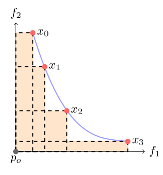
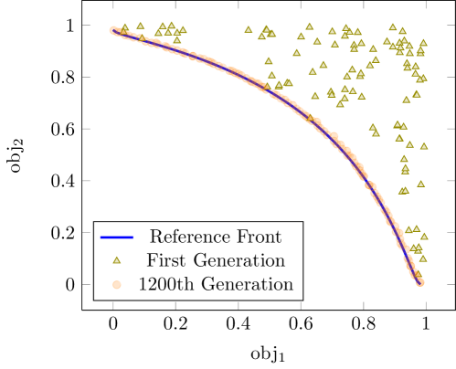
To ensure that the optimizer works correctly, the benchmark problem (4) was solved. To that end, we use a metric for comparing the quality of a Pareto front. Given a point in the Pareto set, we compute the dimensional volume (for objectives) of the dominated space, relative to a chosen origin. This is visualized for objectives in Fig. 4. For further information and details of the implementation see While et al. (2012). Figure 5 and the corresponding hypervolume values in Table 1 show expected convergence. The reference Pareto front is clearly very well approximated. It took a total of 1100 function evaluations to perform this computation. The hypervolume of the reference solution () for our benchmark was computed by sampling the solution provided in Huband et al. (2005).
| tot. function | hypervolume | relative error |
|---|---|---|
| evaluations | ||
| 100 | 0.859753 | |
| 200 | 0.784943 | |
| 500 | 0.685183 | |
| 900 | 0.661898 | |
| 1100 | 0.657615 |
Table 1 shows satisfactory convergence to the sampled reference Pareto front after 1000 (plus the additional 100 evaluations for the initial population) function evaluations.
V.2 AWA Photoinjector Optimization
Next the optimization framework is applied to the high charge beam line at the Argonne Wakefield Accelerator (AWA) facility. The goal of this optimization is to produce beams of electrons that meet design specifications; this includes number of particles (charge), energy, and particle distribution (characterized by beam sizes and energy spread). As shown in Fig. 6, the installed portion of the the beam line consists of an rf photocathode gun, two solenoids, and six linear accelerating cavities followed by four quadrupoles and a stripline kicker. The charge of interest, 40 nC, is needed for two beam acceleration (TBA) experiments performed at the AWA Gai et al. (2012); Jing et al. (2018), which motivates this work. Prior experimental results were limited by beam size when the beam passed through small aperture wakefield structures located downstream. In an attempt to maximize charge transmission in upcoming experiments, magnet strengths of the solenoids and quadrupoles leading into the TBA section of the beam line were optimized, shown in Fig. 7. The simulation model includes from the gun to the septum. The optimization location is chosen as the entrance to the first quadrupole on the dog leg (), see Fig. 7. Minimizing beam sizes here will enable capture and further focusing before space charge effects dominate the beam. This will also enable cleaner transport through downstream elements.


In addition to addressing the challenge of producing an optimized beam, this model was chosen to demonstrate the ability of the framework to tackle large problems. Six design variables and objectives were used, along with three constraints. The objectives include transverse and longitudinal beam sizes, transverse momentum, and longitudinal energy spread. The design variables include the two gun solenoids and the first four quadrupoles strengths. This problem encompasses high dimensionality and nonlinear effects such as space charge. Using this model it was possible to find good solutions that meet the operational goals for the new beamline. One of these solutions is presented in the next section.
V.2.1 Time Step Scan
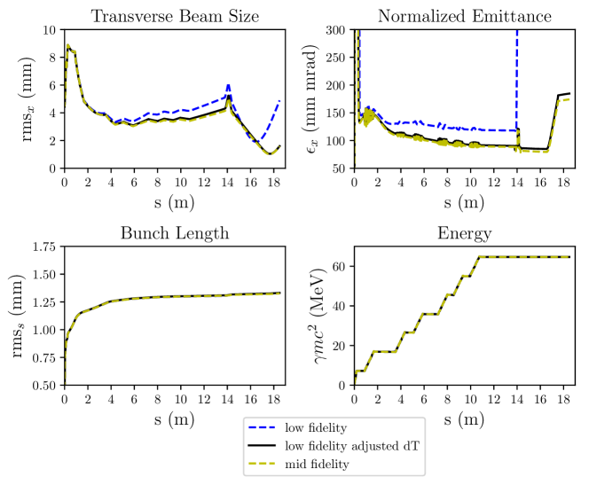
Before running a full scale optimization of the problem described in Subsection V.2, a study on time step and number of particles in the simulation model was done to reduce the time of the simulation while maintaining the physics of interest. The grid size was chosen, and parallelized in the x and y directions. After comparing several options (1,000, 10,000, 20,000, 50,000, 100,000) with a small time step, the number of particles was fixed at 10,000. Next several time steps were explored, see Table 2. The largest steps were too big to resolve the beam parameters accurately. See low fidelity plot in Fig. 8 for results.
| Time Step, dT (s) | Linac | Drift | Quadrupoles |
|---|---|---|---|
| ✗ | ✗ | ✗ | |
| ✗ | ✗ | ✗ | |
| ✗ | ✗ | ✗ | |
| ✓ | ✓ | ✗ | |
| ✓ | ✓ | ✗ | |
| ✓ | ✓ | ✓ |
In the drifts and linac tanks, was sufficient. However, it was not acceptable near the quadrupoles. For all models, the longitudinal parameters (rmss and energy) are calculated correctly, but discrepancies are seen in the transverse (rmsx and ) for low fidelity results. This discrepancy is what led to the decision to adjust the time steps w.r.t. beam line elements. In the linac and drift sections was used. Near sensitive elements such as the quadrupoles, kicker, and septum, a time step of was used. The resulting simulations are low fidelity in most places, but closely approximate the mid fidelity simulations for metrics of interest, as shown in Fig. 8. Mid fidelity simulations used steps of everywhere. The average run time of each simulation with the adjusted time steps was 1.6 minutes. In comparison, the mid fidelity simulation ran for 18 minutes. Note, a smaller time step, , is always used in the gun where the beam has low energy and is changing rapidly.
V.2.2 Hyper parameter Scan
While the optimization problem and goals were well defined (Subsection V.2), it was not clear what the best hyper parameters for the genetic algorithm would be. These parameters include gene mutation probability, mutation probability, recombination probability, number of individuals, and number of generations to complete. Given the beam line in Fig. 6, four small optimization experiments were done with various hyper parameters. Similar to the time step scan, the goal of this exercise was to determine which set of optimization parameters strongly influence the results, and whether there was a time to solution difference. From here on, we will reference each experiment as ex-1, ex-2, ex-3, and ex-4 as shown in Table 3.
| Gene Mutation | Recombination | Number of completed | |
|---|---|---|---|
| Experiment | Probability | Probability | generations |
| ex-1 | 0.1 | 0.9 | 96 |
| ex-2 | 0.3 | 0.7 | 81 |
| ex-3 | 0.8 | 0.2 | 53 |
| ex-4 | 0.01 | 0.09 | 95 |
The maximum number of individuals per generation was fixed at 80. This number was chosen based on the node architecture, and the to prevent a prohibitive computational cost. Each experiment was allowed to run for twenty four hours, with a maximum generation limit of 100. We reduced the six objectives to four, and shortened the simulation time by moving the objectives further upstream to and , the locations before and after the kicker, see Fig. 7. The objectives include: , . The OPAL input file for these cases and all subsequent optimization runs in this paper, can be found at in following repository: https://github.com/nneveu/awa-tba.
After collection of the data for all four experiments, several metrics were compared, including number of generations completed in twenty four hours and Pareto fronts at and , see Fig. 6. From Table 3, we clearly see ex-3 is significantly slower, as it evaluated only 53 generations compared to the experiment with the maximum number, ex-1 at 96 generations. Perhaps this trade off would be acceptable if the Pareto front was significantly improved, but from Fig. 9, but this is not the case. Similar arguments can be made for ex-2, which evaluated about 15 less generations. The Pareto fronts at , are nearly identical. It is expected this trend would continue given more time. When looking at the Pareto front at , only ex-4 has a slightly larger range compared to the others. With ex-2 and ex-3 eliminated due to evaluation time, and a slightly better Pareto front at for ex-4, the hyper parameters in ex-4 were chosen as the default values for subsequent runs.
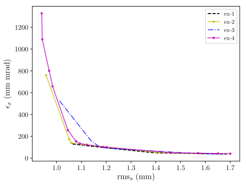
(a) Pareto fronts for ex-1 through ex-4 at .
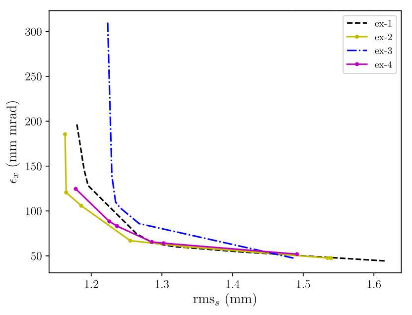
(b) Pareto fronts for ex-1 through ex-4 at .
V.2.3 TBA Optimization Problem
With computational and hyper parameters set, the optimization problem of interest is explored. The objectives (beam sizes and energy spread) are calculated at m, located downstream of the septum, see Fig. 7. Given the longitudinal location of (unless otherwise noted), we define the objectives and input parameters as:
| min | (5) | |||
| (6) | ||||
| (7) | ||||
| constraints | (8) | |||
| (9) | ||||
| (10) | ||||
| subject to | (11) | |||
| (12) | ||||
| (13) | ||||
| (14) | ||||
| (15) | ||||
| (16) |
The first four objectives, parameters (5) to (6), minimize the transverse () beam size and transverse momentum () at the location of interest in the beam line (, see Fig. 7). Minimizing the beam size at this location is essential to to preventing loss of particles by scraping; which ensures better transmission through the wakefield structures downstream. These structures are called Power Extractor and Transfer Structure (PETS), and will be located after the septum and quadrupoles in Fig. 7. This device is putting the tightest constraints on the beam parameters. The aperture diameter is and the bunch length should be below to facilitate large power extraction Gao et al. (2008). Less divergence in the beam (lower transverse momentum spread) reduces growth of transverse beam size after the focal point (location of min beam size). This reduces halo by ensuring the beam is not over focused through a hard waist. The momentum spread is also critical to preventing large growth during transport. All of these factors help with transmission downstream.
The next two objectives in parameter (7) minimize the longitudinal beam size (), and energy spread (dE) at location . This helps reduce the transverse beam size growth in bending elements. A small bunch length () is also critical to the goals of TBA experiments. The power generated in the wakefield structures designed for TBA is related to the bunch length Jing et al. (2018); Gao et al. (2008). Eqs. 8 to 10 define three constraints used to guide the algorithm. However, it is important to not over-constrain the problem, which would prevent the algorithm from converging. The difference constraint, Eq. 10, is used to favor nearly round beams. This prevents one dimension from becoming disproportionately large compared to the other. At the AWA, there is some room in the beam pipe to allow the y dimension to grow, but round beams are preferred. Equations (11) to (16) define the charge, gun voltage, linac voltages, laser radius, gun phase, and linac cavity phases (in that order). These are parameters in the simulation that must be defined, but do not vary during the optimization. For setup of the AWA design variables, objectives, and constraints in the OPAL input file, refer to the the repository above.
Design variables include the currents in two gun solenoids (IBF and IM), and four quadrupole strengths (KQ1-KQ4). The objectives include beam size (transverse and longitudinal), transverse momentum, and energy spread as defined in Eqs. (5) to (7). The location at the entrance of the kicker is (m), and the objectives are optimized at location (m). This is the entrance to the fifth quad in the beam line. This location is where the beam should be captured and focused through subsequent elements.
V.2.4 AWA Optimization Results
All simulations for this experiment were carried out on Bebop a high performance computing (HPC) cluster provided by the Laboratory Computing Resource Center (LCRC) at Argonne National Laboratory (ANL). Intel Knights Landing (KNL) processors at 1.3 GHz with 128 GB of memory and 64 cores per node were used for all runs. There are 352 compute nodes available on Bebop, with a total of 22,528 cores. All jobs were run and compared on 8 cores each, which allowed 8 jobs per node on the KNLs. This in combination with the number of nodes available allows for very large optimization jobs, like the AWA case. Typical runs for this paper used 41 nodes, which corresponds to 2624 KNL cores and a generation size of 328 individuals.
With the time steps and hyper parameters set by the work in Section V.2.1, the optimization problem described in V.2 was run for 200 generations. The initial number of individuals was fixed at 656, and the minimum number individuals in later generations was fixed at 328. These numbers were in part based on the architecture of the KNL’s. Since each simulation takes 8 cores, and there are 64 cores per KNL node, a large population size that would fit evenly on these resources was chosen. Again, the location of optimization is (m).
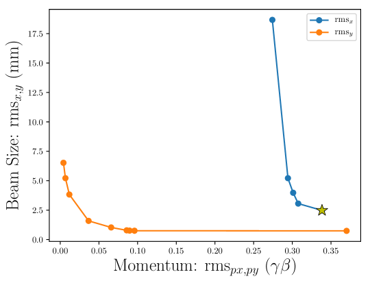
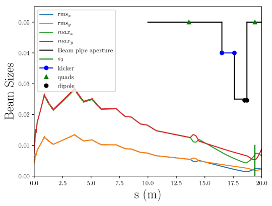
As expected, the x dimension is impacted by the bending elements, and unable to reach the small beam sizes seen in the y dimension. This suggests objectives in the x dimension will drive design variable choices used during operations. However, it is still necessary to include the y dimension in the optimization. Early optimization tests showed the y dimension can easily grow out of control if it is not included in the objectives. Those results are not shown here due to the unfeasible nature of the solutions (i.e. larger than the beam pipe). In the case of bunch length, there are not many options to choose from, as the phase was not varied. With these observations in mind, several beam parameters corresponding to options on the Pareto Front in Fig. 10 were plotted and compared. A select result is shown in Fig. 11. The maximum beam sizes are well below the beam pipe aperture limits, also shown in Fig. 11. The solution is nearly round, which will increase chances of keeping the beam nearly round as it travels to the last triplet in Fig. 7. Overall this solution is satisfactory, and meets all requirements for the new TBA beamline at the AWA.
The TBA line under construction includes a kicker and septum combination to route one bunch train to its own PETS, while the other bunch train is undeflected and goes to a different PETS. The optimization results shown here start at the gun and go through to the first quadrupole after the septum ( (m)). These results were used as the basis for the full solution up to the PETS Neveu (2018). After adjustments to include 3D rf field maps and CSR in the dipoles Neveu (2018), the maximum beam sizes at the PETS location were below 10mm with a bunch length of rmsz = 1.6mm. Although the simulation results at the PETS location cannot yet be verified, since the beamline is not yet completely installed, some checks have been possible for the partially completed beamline. For example, beam images were taken on the YAG screen located downstream of the kicker, and it was found that the extracted beam sizes at different kicker angles were in good agreement with simulation results Neveu (2018). When it becomes possible to test the complete simulation solution, it is expected that there will not be perfect agreement with simulation; for example there may be errors in the fields of beamline elements. However, the simulation can be a tool to track down the source of discrepancies, such as understanding the effect of the gun field on the beam symmetry. More importantly, the optimization results should provide significant improvement in efficiency for achieving a good operational regime.
VI CONCLUSIONS
A general-purpose framework for solving multi-objective optimization problems was presented. Its modular design simplifies the application to simulation-based optimization problems for a wide range of problems and allows to exchange the optimization algorithm. The flexibility of being able to adapt both ends of the optimization process, the forward solver and the optimization algorithm simultaneously not only leads to broad applicability but it facilitates tailoring the optimization strategy to the optimization problem as well.
The framework was integrated into OPAL, and used to study a beam dynamics problem at the AWA. A scan of time step and hyper parameters was done to determine computational settings. Then a full scale physics optimization was performed. Optimization of the 3D beam size and energy spread was accomplished. The TBA beam line presented is currently being installed at the AWA. Once installation is complete, the results shown here will guide future experiments at the AWA.
In contrast to approaches that are tightly coupled to the optimization algorithm, the range of possible applications is much wider. Even in cases where the mathematical model of the forward solver is not known exactly, fixed or real time measurements can be used to guide the search for the Pareto optimal solutions. Finally, combining a multi-objective optimization framework, such as the one presented, with practical experience in the field should expedite the decision making process in the design and operation of particle accelerators.
VII ACKNOWLEDGMENT
The authors thank the AWA team for contributing to the formulation of optimization problems. We gratefully acknowledge the computing resources provided on Bebop, a HPC cluster operated by the LCRC at ANL. Thanks to Scott Doran for providing CAD drawings of the AWA beam lines. This work was partly supported by the U.S. Department of Energy, Office of Science, under contract number DE-AC02-06CH11357 and grant number DE-SC0015479.
References
- Huang (2018) X. Huang, Phys. Rev. Accel. Beams 21, 104601 (2018).
- Hofler et al. (2013) A. Hofler, B. Terzic, M. Kramer, A. Zvezdin, V. Morozov, Y. Roblin, F. Lin, and C. Jarvis, Phys. Rev. ST Accel. Beams 16, 010101 (2013).
- Bazarov and Sinclair (2005) I. V. Bazarov and C. K. Sinclair, Phys. Rev. ST Accel. Beams 8, 034202 (2005).
- Yang et al. (2009) L. Yang, D. Robin, F. Sannibale, C. Steier, and W. Wan, Nucl. Instrum. Methods Phys. Res. A 609, 50 (2009).
- Terzic et al. (2014) B. Terzic, A. S. Hofler, C. J. Reeves, S. A. Khan, G. A. Krafft, J. Benesch, A. Freyberger, and D. Ranjan, Phys. Rev. ST Accel. Beams 17, 101003 (2014).
- Gulliford et al. (2016) C. Gulliford, A. Bartnik, and I. Bazarov, Phys. Rev. Accel. Beams 19, 093402 (2016).
- Gulliford et al. (2017) C. Gulliford, A. Bartnik, I. Bazarov, and J. Maxson, Phys. Rev. Accel. Beams 20, 033401 (2017).
- Kranjčević et al. (2019) M. Kranjčević, A. Adelmann, P. Arbenz, A. Citterio, and L. Stingelin, Nucl. Instrum. Methods Phys. Res. A 920, 106 (2019).
- Physics (2018) P. Physics, “General Particle Tracer (GPT),” (1996-2018), http://www.pulsar.nl/gpt .
- Borland (2018) M. Borland, Elegant: A flexible SDDS-compliant code for accelerator simulation, Tech. Rep. LS-287 (Argonne National Laboratory, 2000-2018).
- Adelmann et al. (2018) A. Adelmann, C. Baumgarten, M. Frey, A. Gsell, V. Rizzoglio, J. Snuverink, C. Metzger-Kraus, Y. Ineichen, S. Russell, C. Wang, S. Sheehy, C. Rogers, and D. Winklehner, The OPAL (Object Oriented Parallel Accelerator Library) Framework, Tech. Rep. PSI-PR-08-02 (Paul Scherrer Institut, 2008-2018).
- Bleuler et al. (2003) S. Bleuler, M. Laumanns, L. Thiele, and E. Zitzler, in Evolutionary Multi-Criterion Optimization, edited by C. M. Fonseca, P. J. Fleming, E. Zitzler, L. Thiele, and K. Deb (Springer, Berlin, Heidelberg, 2003) pp. 494–508.
- Deb (2009) K. Deb, Multi-Objective Optimization Using Evolutionary Algorithms (Wiley, 2009).
- Kirkpatrick et al. (1983) S. Kirkpatrick, C. D. Gelatt, and M. P. Vecchi, Science 220, 671 (1983).
- Kennedy and Eberhart (1995) J. Kennedy and R. Eberhart, in Proc. of ICNN, Vol. 4 (1995) pp. 1942–1948.
- Dorigo et al. (1996) M. Dorigo, V. Maniezzo, and A. Colorni, IEEE Trans. Syst. Man. Cy. B 26, 29 (1996).
- De Castro and Timmis (2002) L. De Castro and J. Timmis, Artificial immune systems: a new computational intelligence approach (Springer, 2002).
- Karaboga (2005) D. Karaboga, Techn. Rep. TR06, Erciyes Univ. Press, Erciyes (2005).
- Shah-Hosseini (2009) H. Shah-Hosseini, Int. J. Bio-Inspir. Com. 1, 71 (2009).
- Deb et al. (2002) K. Deb, A. Pratap, S. Agarwal, and T. Meyarivan, IEEE Trans. Evol. Comp. 6, 182 (2002).
- Filipič and Depolli (2009) B. Filipič and M. Depolli, in Parallel Computing, edited by R. Trobec, M. Vajteršic, and P. Zinterhof (Springer, 2009) pp. 217–240.
- León et al. (2009) C. León, G. Miranda, and C. Segura, Int. J. Artif. Intell. Tools 18, 569 (2009).
- Liefooghe et al. (2007) A. Liefooghe, M. Basseur, L. Jourdan, and E. Talbi, in Evolutionary Multi-Criterion Optimization (Springer, 2007) pp. 386–400.
- Durillo et al. (2006) J. Durillo, A. Nebro, F. Luna, B. Dorronsoro, and E. Alba, jMetal: a java framework for developing multi-objective optimization metaheuristics, Tech. Rep. ITI-2006-10 (University of Málaga, ETSI Informática, Campus de Teatinos, 2006).
- Arbenz and Chinellato (2008) P. Arbenz and O. Chinellato, Appl. Numer. Math. 58, 381 (2008).
- boo (2015) “The Boost Spirit Home Page,” (2015), http://boost-spirit.com/.
- E. Friedman and I. Maman (2003) E. Friedman and I. Maman , “Chapter 45. Boost.Variant,” (2003), www.boost.org/doc/html/variant.html.
- Gregor (2004) D. Gregor, “Chapter 15. Boost.Function,” (2004), www.boost.org/libs/function/.
- Balaji et al. (2009) P. Balaji, A. Chan, R. Thakur, W. Gropp, and E. L. Lusk, Computer Science - Research and Development 24, 11 (2009).
- Boyd et al. (2006) S. Boyd, A. Ghosh, B. Prabhakar, and D. Shah, IEEE Trans. Inform. Theory 52, 2508 (2006).
- Aysal et al. (2009) T. Aysal, M. Yildiz, A. Sarwate, and A. Scaglione, IEEE Trans. Signal Process. 57, 2748 (2009).
- Huband et al. (2005) S. Huband, L. Barone, L. While, and P. Hingston, in Proc. of Intl. Conf. Evol. Multi-Criterion Optimization (Springer-Verlag, Berlin, Heidelberg, 2005) pp. 280–295.
- While et al. (2012) L. While, L. Bradstreet, and L. Barone, IEEE Trans. Evol. Comput. 16, 86 (2012).
- Gai et al. (2012) W. Gai, J. G. Power, and C. Jing, Journal of Plasma Physics 78, 339–345 (2012).
- Jing et al. (2018) C. Jing et al., Nucl. Instrum. Methods Phys. Res. A 898, 72 (2018).
- Gao et al. (2008) F. Gao, M. E. Conde, W. Gai, C. Jing, R. Konecny, W. Liu, J. G. Power, T. Wong, and Z. Yusof, Phys. Rev. ST Accel. Beams 11, 041301 (2008).
- Neveu (2018) N. Neveu, Beam Line Design for Fully Staged Two Beam Acceleration at the Argonne Wakefield Accelerator Facility, Ph.D. thesis, Illinois Institute of Technology (2018).