Analytically solvable model of an electronic Mach-Zehnder interferometer

Abstract

We consider a class of models of non-equilibrium electronic Mach-Zehnder interferometers built on integer quantum Hall edges states. The models are characterized by the electron-electron interaction being restricted to the inner part of the interferometer and transmission coefficients of the quantum quantum point contacts, defining the interferometer, which may take arbitrary values from zero to one. We establish an exact solution of these models in terms of single-particle quantities—determinants and resolvents of Fredholm integral operators. In the general situation, the results can be obtained numerically. In the case of strong charging interaction, the operators acquire the block Toeplitz form. Analyzing the corresponding Riemann-Hilbert problem, we reduce the result to certain singular single-channel determinants (which are a generalization of Toeplitz determinants with Fisher-Hartwig singularities), and obtain an analytic result for the interference current (and, in particular, for the visibility of Aharonov-Bohm oscillations). Our results, which are in good agreement with experimental observations, show an intimate connection between the observed “lobe” structure in the visibility of Aharonov-Bohm oscillations and multiple branches in the asymptotics of singular integral determinants.

I Introduction

Electronic Mach-Zehnder interferometers (MZIs) realized with edge states in the integer quantum Hall (QH) regime have attracted a lot of attention recently because of a striking interplay between the quantum coherence and effects of electron-electron interaction observed in these mesoscopic devices Ji et al. (2003); Neder et al. (2006, 2007a, 2007b); Roulleau et al. (2007, 2008a, 2008b, 2009); Litvin et al. (2007, 2008, 2010); Bieri et al. (2009); Huynh et al. (2012); Helzel et al. (2012). By analogy to the optical interferometer, the chiral edge states in the electronic MZI, playing the role of light beams, are coupled by quantum point contacts (QPCs), which act as electron beam-splitters (see Fig. 1). The differential conductance measured in the above experiments shows strong Aharonov-Bohm (AB) oscillations. They are a manifestation of quantum coherence of electrons, propagating through different arms of interferometer, and are quantified in terms of visibility. The most remarkable experimental observation is that the out-of-equilibrium visibility does not decrease monotonically with voltage but rather demonstrates a sequence of decaying oscillations (“lobes”). Such a dependence cannot be explained within an assumption of non-interacting electrons.

Investigation of quantum interference and decoherence in Aharonov-Bohm rings and interferometers has a long history Aronov and Sharvin (1987). In particular, much attention has been paid to sources of dephasing that may arise from the external noise Seelig and Büttiker (2001); Seelig et al. (2003); Marquardt and Bruder (2004a, b); Förster et al. (2005); Neder and Marquardt (2007) or are the result of the intrinsic electron-electron interaction Ludwig and Mirlin (2004); Le Hur (2005, 2006); Texier and Montambaux (2005); Dmitriev et al. (2010). The advent of QH interferometers has renewed the interest in this problem, with a considerable number of recent theoretical works Chalker et al. (2007); Sukhorukov and Cheianov (2007); Neder and Ginossar (2008); Youn et al. (2008); Levkivskyi and Sukhorukov (2008, 2009); Kovrizhin and Chalker (2009, 2010); Schneider et al. (2011); Rufino et al. (2012) aiming at a resolution of the “visibility puzzle” in MZIs. These recent theories can be subdivided into the approaches assuming contact Levkivskyi and Sukhorukov (2008, 2009); Rufino et al. (2012) and long-range Chalker et al. (2007); Sukhorukov and Cheianov (2007); Kovrizhin and Chalker (2009, 2010); Schneider et al. (2011) Coulomb interaction. Despite the fact that the model of contact e-e interaction may successfully describe the related experiments on the energy relaxation in the QH edge states at filling factor $\nu$=2 Altimiras et al. (2010a, b); le Sueur et al. (2010); Kovrizhin and Chalker (2012); Levkivskyi and Sukhorukov (2012), results of Refs. Schneider et al., 2011; Rufino et al., 2012 indicate that the account of the long-range character of Coulomb interaction is of central importance for a full understanding of non-equilibrium phenomena in MZIs.

The natural choice of a theoretical approach to one-dimensional (1D) interacting electrons in the QH edge states is that of bosonization Wen (2004). However, in the case under interest, one faces serious complications when trying to apply this approach. First, already in the single-channel problem, the bosonized action of the theory ceases to be Gaussian under non-equilibrium conditions Gutman et al. (2008, 2010a, 2010b) (see also a related earlier work D.A.Abanin and Levitov (2005) on the non-equilibrium Fermi-edge singularity). This difficulty has been solved by development of the non-equilibrium bosonization formalism yielding results for physical observables in terms of single-particle Fredholm determinants which are of Toeplitz type for a short-range interaction modelGutman et al. (2010a, b). Second, an even more severe obstacle arises when one describes electron scattering at QPCs. Specifically, electron tunneling between two edge channels yields the $\cos$-like term in the bosonized Hamiltonian (an the action), impeding a solution to the problem. For this reason, almost all recent theories of MZIs consider the limit of weakly coupled edge states where the perturbative treatment of electron tunneling at QPCs is justified. This is rather unfortunate since in the experiment transmission coefficients of both QPCs are usually close to one half. While in a very restricted set of models exact solutions via the Bethe ansatz are available Fendley et al. (1995); Ponomarenko and Averin (2009, 2010), the systems we are interested in do not belong to this class. On the other hand, it would be clearly highly advantageous to have an analytically treatable mode for integer QH MZI for an arbitrary number of edge channels, arbitrary interaction range and strength, and arbitrary transmissions at QPC.

In this paper we consider the model of the MZI operating at integer filling factor $\nu$ where electrons interact only when they are inside the interferometer. The model is specified by two single-particle scattering matrices of the QPCs defining the interferometer and by the model of Coulomb interaction inside the interferometer. We focus on the model of “maximally long-range” interaction when the interaction energy depends only on total charges collected within each of the arms and is characterized by an electrostatic charging energy $E_{c}$. Let us emphasize that this restriction is not crucial: within this approach one can, in principle, consider any interaction within the interior region of MZI.

For the case $\nu=1$, such a model was introduced in Refs. Neder and Ginossar, 2008; Youn et al., 2008. In Ref. Kovrizhin and Chalker, 2010 an exact solution to it at $\nu=1$ was obtained by using a combination of bosonization and refermionization techniques and was expressed in terms of single-particle determinant and resolvent that were evaluated numerically. Our way to treat the problem is different in many aspects. We consider a MZI with an arbitrary number of edge states and use the non-equilibrium functional bosonization approach developed by us previously Ngo Dinh et al. (2012). Within this framework we demonstrate that an interfering current can be expressed in terms of a Fredholm functional determinant of the single-particle “counting” operator which bears resemblance to the problem of electron full counting statistics (FCS) of mesoscopic transport Levitov et al. (1996). In general, this determinant should be evaluated numerically. In the limit of strong interaction $E_{c}\gg 1/\tau$, where $\tau$ is the electron flight time through the MZI, the “counting” operator takes the block Toeplitz form. Under this condition, a fully analytical treatment turns out to be possible. By solving the Riemann-Hilbert problem, we get rid of the matrix structure and express the result in terms of a determinant of a single-channel singular integral operator generalizing Toeplitz determinants with Fisher-Hartwig singularities. Determinants of this type have been studied in Ref. Protopopov et al., 2012 where a conjecture on their asymptotic behavior was formulated and supported by a large body of analytical and numerical arguments. This allows us to obtain the result in a closed analytic form.

Our analytical result demonstrates that the “lobe” pattern in visibility is a many-body interference effect resulting from the quantum superposition of (at least) two many-particle scattering amplitudes with the mutual phase difference which is linear in voltage. In the limit of strong interaction we find the scaling exponents which describe power-law dependences of these amplitudes on voltage and obtain the non-equilibrium dephasing rate governing the exponential suppression of visibility with bias (or, equivalently, with the length of the arms of the MZI). The power-law exponents as well as the dephasing rate depend on the transmission coefficient of the first QPC and on the filling factor $\nu$.

Our analytical findings are corroborated and complemented by numerical evaluations of the Fredholm determinants determining the exact solution for arbitrary $E_{c}\sim 1/\tau$. At $E_{c}\gg 1/\tau$ our numerical results provide further support to the aforementioned conjecture of Ref. Protopopov et al., 2012. At moderate charging energy $E_{c}\gtrsim 1/\tau$ and $\nu$=2 the obtained results match very well experimental observations.

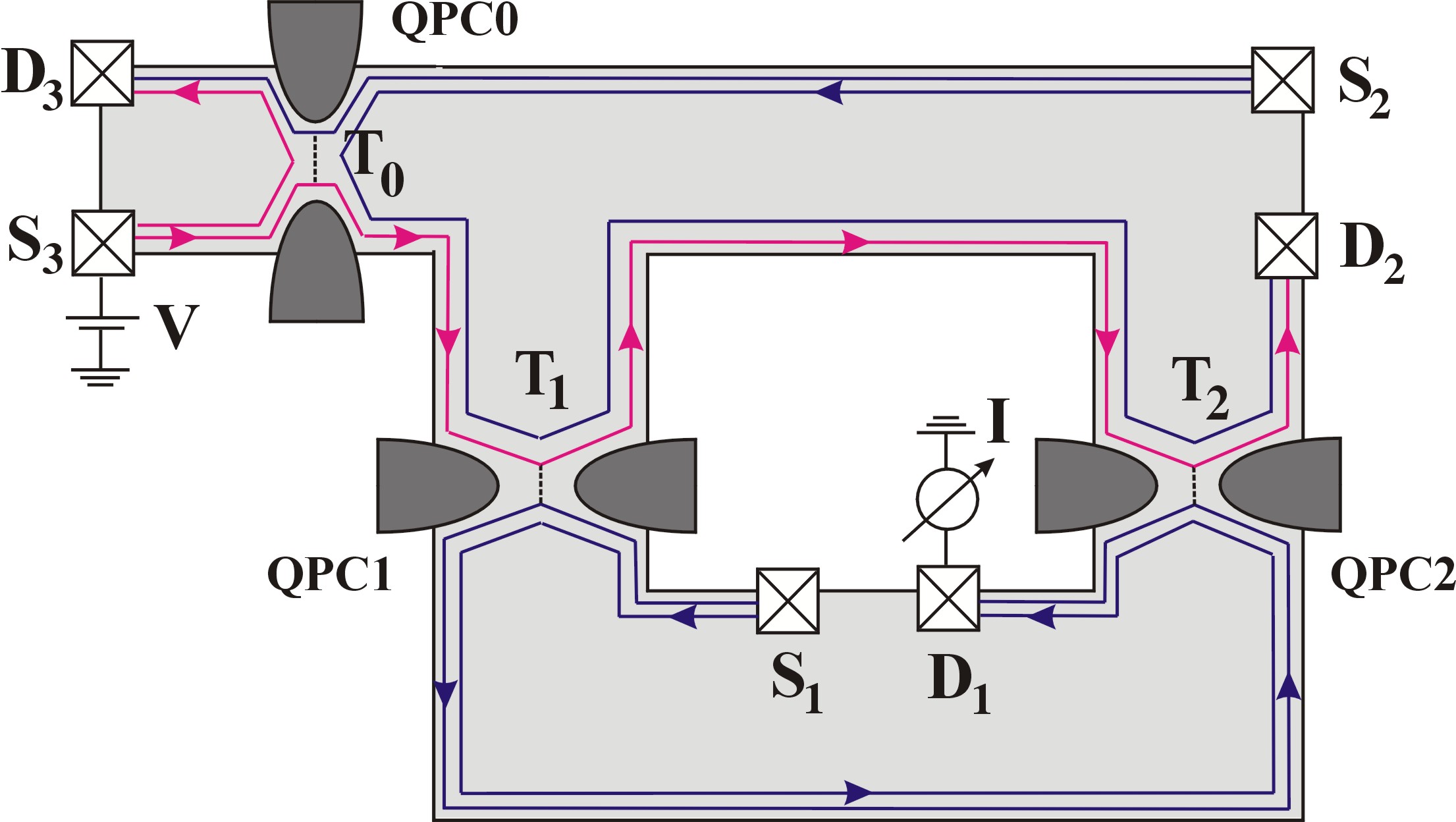
Figure 1: Layout of an electronic Mach-Zehnder interferometer built on quantum-Hall edge states at filling factor $\nu=2$. Quantum point contact (QPC1 and QPC2) characterized by transparencies $T_{1(2)}$ are used to partially mix the outer edge channels. All Ohmic contacts are grounded, except for the source terminal $S_{3}$ which is kept at voltage $V$. The current is measured in the drain terminal $D_{1}$. The QPC0 can be used to dilute the incoming current in the outer channel by changing the transparency $T_{0}$.

The remainder of the paper is organized as follows. Section II is devoted to the exposition of our main results and their physical interpretation. In Sec. III we present the non-equilibrium functional bosonization approach. We demonstrate that the MZI problem defined above is exactly solvable by means of the instanton method. In the limit of strong interaction (Sec. IV), the full analytical treatment becomes possible. It is based upon the asymptotic results for the generalized Toeplitz determinants. We show the relation of the MZI problem to the latter theory and evaluate analytically the Aharonov-Bohm conductance. In Sec. V we consider the influence of an additional quantum point contact (QPC0) diluting the incoming current in one of the channels and develop numerically exact approach to solve the problem in the case of a moderate charging energy. Finally, in Sec. VI we summarize the findings of this work and discuss prospects for future research.

II Results and qualitative discussion

In this section we set the stage by defining the theoretical model of the Mach-Zehnder interferometer and then present our results and give their physical interpretation. This part of the paper is self-contained and can be read independently of other sections, where we provide technical details of the calculations.

II.1 Model of the MZI

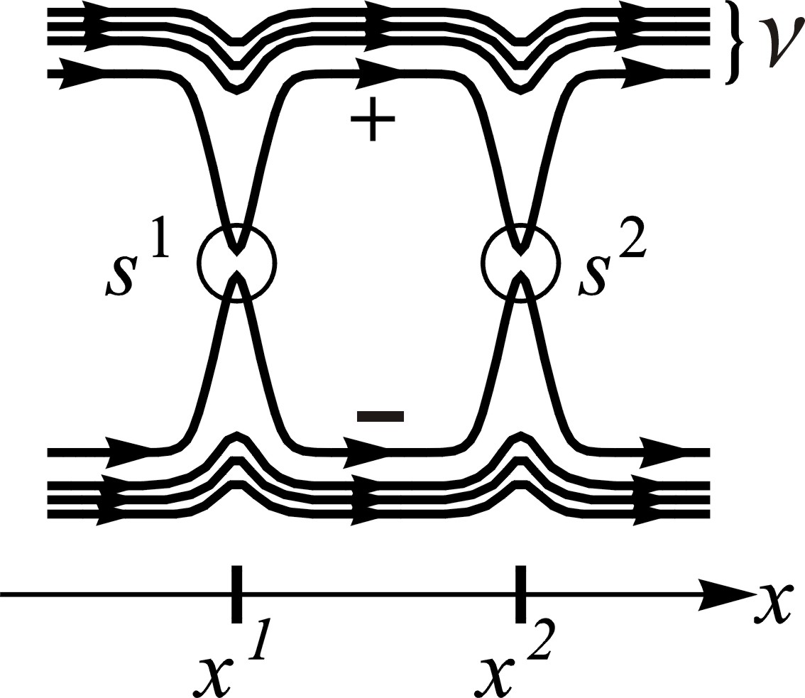
Figure 2: Scheme of an MZI at filling factor $\nu$. Two quantum point contacts are characterized by the scattering matrices $s^{1}$ and $s^{2}$, which connect the outer channels. Inner channels are fully reflected.

We consider the Mach-Zehnder interferometer (MZI) realized with edge states in the QH regime at integer filling factor $\nu$. The experimental layout (in case of $\nu=2$) and the scheme of the MZI are shown in Figs. 1 and 2. In this setup the outer chiral channels, propagating along different arms of the MZI (we denote them by the index $\pm$) are coupled by means of two quantum point contacts (QPCs), located at points $x_{\pm}^{1(2)}$. An additional quantum point contact, QPC0, is used to bias the incoming outer channel at the upper edge by voltage $V$ (and in general also to dilute the incoming current if the transmission coefficient of the QPC0 is tuned to a value $T_{0}>0$). We further assume that all inner chiral channels are fully reflected from each QPC and, in particular, the incoming inner channels are grounded. This layout of the MZI and the bias scheme are realized in most of the experiments (an exception is Ref. Bieri et al., 2009, where the MZI setup at $\nu=2$ did not contain additional QPC0).

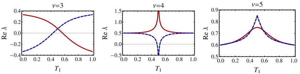
Figure 3: Power-law exponents shown as the function of transmission coefficient $T_{1}$. Solid line shows ${\rm Re}\,\lambda_{1}$, dashed line shows ${\rm Re}\,\lambda_{2}$ in the case of $\nu=3$, and $(-{\rm Re}\,\lambda_{2})$ in the case of $\nu=4,5$.

A theoretical model considered throughout the paper is specified by the action ${\cal S}={\cal S}_{0}+{\cal S}_{\rm int}$ of interacting 1D fermions,

$${\cal S}_{0} = \sum_{\varrho=\pm}\int dt\,dx\,\bar{\psi}_{\varrho}(x)\left(i\partial_{t}+iv\partial_{x}\right)\psi_{\varrho}(x),$$ (1)

$${\cal S}_{\rm int} = \frac{1}{2}E_{c}\sum_{\varrho=\pm}\int dt\,{\cal N}_{\varrho}^{\,2},$$ (2)

which are described by the Grassmann fields $\psi_{\varrho}$ in the arm $\varrho=\pm$. In the case $\nu\geq 2$ the fermionic fields have the vector structure $\psi_{\varrho}=(\psi_{1\varrho},\dots,\psi_{\nu\varrho})^{T}$ due to multiple edge channels. The Coulomb interaction is taken into account by the electrostatic model with a charging energy $E_{c}=e^{2}/C$, such that electrons interact only when they are inside the interferometer. Thus in Eq. (2)

$${\cal N}_{\varrho}=\sum_{k=1}^{\nu}\int_{x_{\varrho}^{1}}^{x_{\varrho}^{2}}\bar{\psi}_{k\varrho}(x+0)\psi_{k\varrho}(x)$$ (3)

is the total number of electrons in the upper/lower arm of the MZI. The action ${\cal A}_{\rm int}$ describes intra- and interchannel Coulomb interaction which is maximally non-local (or long-range) in space. At the same time the inter-edge interaction is disregarded in our model, which is motivated by the fact that different edges are spatially well separated. At the QPCs outgoing fermion fields (with channel index $k=1$) are related to the incoming ones by the scattering matrices

$$\psi_{1\varrho}(x_{\varrho}^{j}+0)=s_{\varrho\mu}^{j}\psi_{1\mu}(x_{\mu}^{j}-0),$$ (4)

$$\hat{s}^{j}=\left(\begin{array}[]{cc}iR_{j}^{1/2}&T_{j}^{1/2}\\ T_{j}^{1/2}&iR_{j}^{1/2}\end{array}\right),$$ (7)

where $T_{j}$ and $R_{j}$ are reflection and transmission coefficients at the $j$-th QPC.

The model of the MZI with the above action ${\cal A}$ is exactly solvable for any value of the charging energy $E_{c}$ and transmission coefficients $T_{j}$, as we show in Sections III, IV and V. For simplicity, we consider an interferometer with equal arms, $x_{+}^{(2)}-x_{+}^{(1)}=x_{-}^{(2)}-x_{-}^{(1)}=L$, which is predominantly the experimental situation. In the limit $E_{c}\tau\gg 1$, where $\tau=L/v$ is the electron dwell time in the MZI, fully analytical treatment is possible. In the more general case $E_{c}\tau\sim 1$ we have developed a numerically exact scheme to evaluate the visibility in the MZI as a function of voltage (Sec. V). Before going into details of the calculations (Sec. III), we summarize our main results.

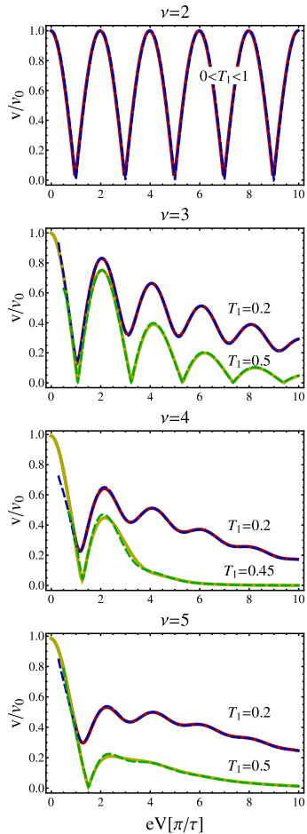
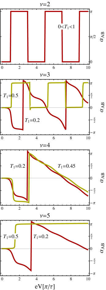
Figure 4: The voltage dependence of the visibility (normalized to its non-interacting value; left) and of the phase (right) of AB oscillations for $\nu=2,3,4,5$ in the strong-interaction limit, $E_{c}\tau\gg 1$. Solid lines show numerically exact results, dashed lines represent analytical results. The latter are strictly speaking valid in the asymptotic high-voltage limit $eV\tau\gg 1$ but turn out to work almost perfectly already at very modest values of voltages, $eV\tau/\pi\gtrsim 0.5$.

II.2 Limit of strong interaction

First, we discuss the results in the limit $E_{c}\tau\gg 1$. In the case of not too low voltages, namely at $eV\tau\gtrsim~{}1$, our model predicts the asymptotic expansion for the differential conductance $dI/dV$ of the MZI in the form

$${\cal G}(V) = \frac{e^{2}}{2\pi\hbar}\Bigl{(}T_{1}R_{2}+T_{2}R_{1}$$ (8)

$$+ 2(T_{1}R_{1}T_{2}R_{2})^{1/2}{\rm Re}\left[e^{i\Phi}\frac{\partial{\cal I}_{0}}{\partial(eV\tau)}\right]\Bigr{)},$$

where $\Phi$ is the magnetic flux and ${\cal I}_{0}$ is the amplitude of the interference Aharonov-Bohm (AB) contribution to the current,

$${\cal I}_{0}=e^{ieV\tau(\beta_{1}+1/\nu)}\Bigl{(}C_{1}(eV\tau)^{\lambda_{1}}+C_{2}(eV\tau)^{\lambda_{2}}e^{\pm ieV\tau}\Bigr{)}.$$ (9)

The choice of the sign $\pm$ in the exponent of the last term will be explained below Eq. (15). Equation (9) contains the two leading terms of a series (in general, infinite). The dependence of each term of this series on $eV\tau$ is characterized by a certain power-law exponent $\lambda_{i}$ and by a certain oscillating factor.

Interpretation of the different ingredients in this expression is as follows. The coefficient

$$\beta_{1}=\frac{1}{2\pi i}\ln\left(R_{1}e^{-4\pi i/\nu}+T_{1}\right)$$ (10)

describes the non-equilibrium dephasing of the AB oscillations induced by a combined effect of inelastic e-e scattering and the quantum shot noise generated at the 1st QPC. If $\nu\geq 3$ then ${\rm Im}\beta_{1}>0$ and, by defining the out-of-equilibrium dephasing rate as

$$\tau_{\phi}^{-1}=eV\,{\rm Im}\,\beta_{1},$$ (11)

we see that AB oscillations are suppressed by the factor $e^{-\tau/\tau_{\phi}}$ in the high-bias limit $eV\gg 1/\tau$.

It is worth stressing that the exponential suppression of the interference current is directly related to the full counting statistics (FCS) of electrons passing through the QPC1 at the time interval $\tau$. Indeed, defining the FCS cumulant generating function (CGF) of the backscattering current as

$$\chi_{\tau}(\lambda)=\left[1+R_{1}(e^{i\lambda}-1)\right]^{eV\tau/2\pi},$$ (12)

where $\lambda$ is the so-called “counting field” Levitov et al. (1996), we see that the damping factor is equal to

$$e^{i\beta_{1}eV\tau}=\chi_{\tau}(-4\pi/\nu).$$ (13)

The exponents $\lambda_{1,2}$, which set the power-law dependence of the interference current on bias, belong to the class of non-equilibrium quantum critical exponents. Physically, they can be understood as being due to the Anderson orthogonality catastrophe which happens each time when an electron enters or leaves the interior part of the MZI where it strongly interacts with all other electrons. It is worth mentioning that in the considered simplified model, where the e-e interaction is present only inside MZI, the orthogonality catastrophe is absent for the incoherent contribution to the current, which stays linear in voltage as in the case of non-interacting fermions.

The exponents $\lambda_{1,2}$ are functions of both, the filling factor $\nu$ and the transparency $T_{1}$ of the first QPC, and are shown in Fig. 3. The explicit expressions read

$$\lambda_{1,2}= - 2\Bigl{(}\frac{1}{\nu}-\frac{1}{2}+\beta_{1}\pm\frac{1}{2}\Bigr{)}^{2}$$

$$+ 1-\frac{2}{\nu}+\frac{2}{\nu^{2}},\qquad 2\leq\nu<4,$$

for low filling factors and

$$\lambda_{1} = -2\Bigl{(}\frac{1}{\nu}+\beta_{1}\Bigr{)}^{2}+1-\frac{2}{\nu}+\frac{2}{\nu^{2}},$$ (15)

$$\lambda_{2} = -2\Bigl{(}\frac{1}{\nu}+\beta_{1}\pm\frac{1}{2}\Bigr{)}^{2}-\frac{1}{2}+\frac{2}{\nu^{2}},\quad\nu\geq 4$$

in the case of higher $\nu$. In the case $2\leq\nu<4$ the voltage dependent phase factor in Eq. (9) has to be taken with the sign (+). For $\nu\geq 4$ the $\pm$ sign corresponds to the case $T_{1}>1/2$ and $T_{1}<1/2$, respectively. The coefficients $C_{1,2}$ in Eq. (9) are some bias-independent complex numbers which depend solely on $\nu$ and $T_{1}$ and can be found from the fit of this asymptotic expansion to its numerically exact counterpart. In the limit of strong interaction, $E_{c}\tau\gg 1$, the case $\nu=1$ is very special. Specifically, one has then ${\cal I}_{0}=(eV\tau)$ and the MZI behavior is the same as in the absence of e-e interaction.

Experimentally, one usually quantifies the coherence of the interferometer in terms of the visibility ${\cal V}$ and the phase $\alpha_{AB}$ of the AB oscillations of the conductance. The visibility is defined as the ratio of the amplitude of the AB oscillations to the mean value of the conductance. In our model

$${\cal V}={\cal V}_{0}\frac{\partial\,{\cal I}_{0}}{\partial(eV\tau)},\quad{\cal V}_{0}=\frac{2(T_{1}R_{1}T_{2}R_{2})^{1/2}}{T_{1}R_{2}+T_{2}R_{1}},$$ (16)

where ${\cal V}_{0}$ is the non-interacting value of ${\cal V}$, and

$$\alpha_{AB}={\rm arg}\left[{\partial\,{\cal I}_{0}}/{\partial(eV\tau)}\right].$$ (17)

In terms of the above quantities the conductance ${\cal G}(V)$ takes the form

$${\cal G}(V)=\frac{e^{2}}{2\pi\hbar}\Bigl{(}R_{1}T_{2}+R_{2}T_{1}\Bigr{)}\Bigl{(}1+{\cal V}(V)\cos\bigl{[}\Phi+\alpha_{AB}(V)\bigr{]}\Bigr{)}.$$ (18)

In Fig. 4 we show the visibility ${\cal V}$ (normalized to its non-interacting value ${\cal V}_{0}$) and the phase $\alpha_{\rm AB}$ of the AB oscillations as functions of bias for different filling factors $\nu=2,3,4,5$ and for different transmissions $T_{1}$.

In each plot we have fitted the exact visibility (obtained numerically) by its analytic form based on Eq. (9) with two free parameters $C_{1}$ and $C_{2}$. Although Eq. (9) is strictly speaking an asymptotic formula valid in the high voltage limit $eV\tau\gg 1$, we see in Fig. 4 that the analytical result is an excellent approximation already starting from very modest values of voltages, $eV\tau/\pi\gtrsim 0.5$. For still smaller voltages, the visibility saturates at its non-interacting value ${\cal V}_{0}$.

The most spectacular feature of Fig. 4 are oscillations of visibility which become particularly strong yielding a “lobe structure with the visibility reaching zero at minima for $\nu=2$ (for any value of $T_{1}$) and for $T_{1}=0.5$ (for any $\nu$). In this cases, the cusps in the visibility at its minima are accompanied by $\pi$-jumps in the phase $\alpha_{\rm AB}$. As we explain below, the special role of $\nu=2$ is a characteristic feature of the strong-interaction limit. On the other hand, the point $T_{1}=0.5$ remains special for a generic interaction.

At $\nu=2$ we have $\lambda_{1}=\lambda_{2}=0$ and $C_{1}=-C_{2}$. This gives the oscillatory visibility ${\cal V}={\cal V}_{0}\cos(eV\tau/2)$ which is independent of the transparency $T_{1}$ and does not decay with bias. The behavior of the MZI in this case is analogous to that in a model with short-range electron interaction which is also exactly solvable at $\nu=2$ by means of the method of refermionization, as has been recently shown in Ref. Rufino et al., 2012. On a technical level, the absence of dephasing and independence of visibility on $T_{1}$ at $\nu=2$ in the limit $E_{c}\tau\gg 1$ comes from the fact that the counting phase becomes $-4\pi/\nu=-2\pi$ in this case. At a moderate charging energy $E_{c}\tau\sim 1$ both the dephasing and the dependence on $T_{1}$ in the visibility of $\nu=2$ MZI are restored, see Sec. II.3.

In the case $\nu=3$ an infinite number of lobes is observed. As discussed above, the visibility reaches zero at minima when (and only when) the transmission is $T_{1}=1/2$. The reason for this special role of the point $T=1/2$ is as follows: in this case the real parts of the two exponents are equal, $\mathrm{Re}\,\lambda_{1}=\mathrm{Re}\,\lambda_{2}$.

For $\nu\geq 4$ our model predicts only one central and one side lobe. Note, that at $\nu=4$ the exponents $\lambda_{1,2}$ logarithmically diverge at $T_{1}\to 1/2$. This is the reason why at $\nu=4$ we have chosen to plot ${\cal V}(V)$ and $\alpha_{AB}(V)$ for a slightly different value $T_{1}=0.45$ (see Fig. 4).

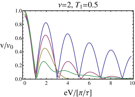
Figure 5: Visibility of AB oscillation at $\nu=2$, $T_{1}=0.5$, and strong interaction, $E_{c}\tau\gg 1$, in the presence of an additional quantum point contact, QPC0. The curves from up to down were evaluated numerically for the reflection coefficient of QPC0 equal to $R_{0}=0.9,0.7,0.5$ and $0.3$.

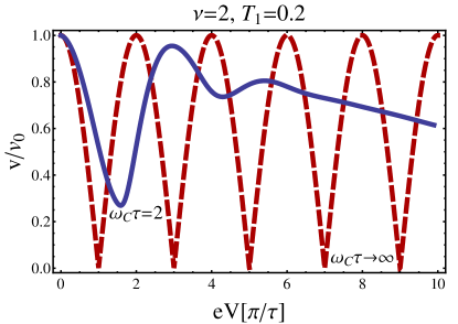
Figure 6: Bias dependence of visibility of MZI with $\nu=2$ for the moderate interaction strength ($\omega_{c}\tau=2$, solid blue curve) in comparison to the limit of strong interaction ($\omega_{c}\tau\to\infty$, dashed red line), where $\omega_{c}=\nu E_{c}/\pi$ is the charge relaxation frequency. Note that at finite $\omega_{c}$ the nodes in visibility are present only at $T_{1}=1/2$.

We turn now to the effect of a dilution of the impinging current due to the electron scattering at an additional quantum point contact, QPC0, which is put outside of the interferometer. At $R_{0}<1$ the QPC0 generates the double-step distribution function $f_{+}(\epsilon)=T_{0}\theta(-\epsilon)+R_{0}\theta(eV-\epsilon)$ for incoming electrons, which affects the power-law exponent and serves as an additional source of dephasing. The effect of QPC0 is particularly noticeable in the strong-interaction model with $\nu=2$, since in this situation no dephasing and no power-law decay of oscillations is found in the absence of QPC0 (see above). In Fig. 5 we show the visibility in this situation, with half-transmitting QPC1, $T_{1}=1/2$, and for different values of the reflection coefficient $R_{0}$ of QPC0. In the case $R_{0}>1/2$ the suppression of visibility with voltage can be roughly characterized by the dephasing rate $1/\tau_{\phi}=(eV/2\pi)\ln(2R_{0}-1)$, which diverges logarithmically at $R_{0}\to 1/2$. At this value of $R_{0}$ the behavior of the MZI visibility changes from the regime with multiple side lobes, characterized by periodic oscillations in ${\cal V}(V)$ with a typical period $\sim 2\pi/\tau$, to the regime with only one node. Such a transition in the behavior of visibility under variation of $R_{0}$ has been first found in Ref. Levkivskyi and Sukhorukov, 2009 in the weak-tunneling regime $T_{1}\ll 1$ for the short-range e-e interaction model. Recently, such an effect of QPC0 on the visibility was observed experimentallyHelzel et al. (2012). We believe that the experimental conditions of long-range interaction and $T_{1}\approx 1/2$ are closer to the ones studied within our model.

As discussed in more detail Sec. IV.3.3 the appearance of the visibility fringes in our model stems from the superposition of two multi-particle amplitudes having the relative phase shift $eV\tau$. These amplitudes correspond to processes with different number of particle-hole excitations between two Fermi edges. In other words, the “lobe” pattern in the visibility is a many-body effect linked to e-e interaction.

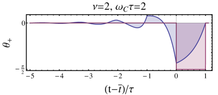
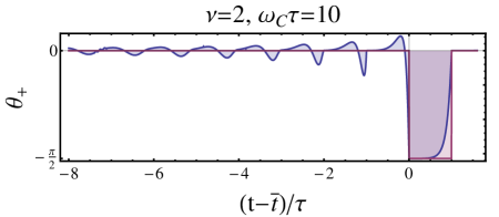
Figure 7: Time-dependent “counting” phase for $\nu=2$ and two strengths of Coulomb interaction, $\omega_{c}\tau=2$ and $\omega_{c}\tau=10$, where $\omega_{c}=\nu E_{c}/\pi$ is the charge relaxation frequency. The phase approaches the “window” function, Eq. (23), in the strong-interaction limit $E_{c}\to\infty$.

II.3 The case of moderate strength of interaction

In this subsection we discuss the results for visibility in the case of not too strong e-e interaction, $E_{c}\tau\sim 1$. We consider here only the case $\nu=2$ for the following two reasons. First, the majority of experimental data for MZIs has been collected for this filling factor. Second, contrary to higher filling factors, at $\nu=2$ a finite (rather than infinite) value of $E_{c}\tau$ changes the result qualitatively, since there is no dephasing and no $T_{1}$ dependence at $E_{c}\tau\to\infty$.

The numerically calculated plots of visibility for transparencies $T_{1}=0.5$ and $T_{1}=0.2$ are shown in Fig. 6. It is seen that the finite charging energy $E_{c}$ gives rise to the decay of visibility ${\cal V}(V)$ with bias contrary to its behavior at $E_{c}\tau\to\infty$ discussed in the previous subsection II.2. Note also that nodes (zero-visibility points) in ${\cal V}(V)$ are generally present only in the case $T_{1}=1/2$. At the transmission coefficient close (but not equal) to one half the nodes are superseded by deep minima. Further, the period of oscillations increases with decreasing $E_{c}$. However, the estimate $e(\Delta V)\sim 2\pi/\tau$ for the scale of oscillations remains valid up to the moderate charging energy $E_{c}\sim 1/\tau$. As an example, Fig. 6 shows that at $E_{c}\tau=\pi$ the period is larger than its strong-interaction limiting value $e(\Delta V)=2\pi/\tau$ by a factor $\simeq 1.5$.

The dephasing rate $1/\tau_{\phi}$ describing the exponential suppression ($\propto e^{-\tau/\tau_{\phi}}$) of the visibility with bias is found to be

$$\tau_{\phi}^{-1}=-\frac{eV}{2\pi\tau}\int_{-\infty}^{\tau+\bar{t}}\,{\rm Re}\Bigl{[}\ln\left(1+R_{1}(e^{4i\theta_{+}(t)}-1)\right)\Bigr{]}\,dt,$$ (19)

where $\bar{t}$ is the time when the electron enters the interferometer and $\theta_{+}(t)$ is the time-dependent “counting” phase given by

$$\theta_{+}(t)=-{1\over\nu}{\rm Im}\left[J^{>}(\bar{t}-t)-J^{>}(\tau-t+\bar{t})\right],$$ (20)

with the function $J^{>}(t)$ defined below in Eq. (55). The phase $\theta_{+}(t)$ is shown in Fig. 7 for $\omega_{c}\tau=2$ and $\omega_{c}\tau=10$. In the limit $E_{c}\tau\gg 1$ the time dependence of $\theta_{+}(t)$ approaches the “window” function

$$\theta_{+}(t)=\left\{\begin{array}[]{ccl}-\pi/\nu,&&t\in[\bar{t},\bar{t}+\tau]\\ 0,&&t\notin[\bar{t},\bar{t}+\tau],\end{array}\right.$$ (23)

causing the dephasing rate to vanish at $\nu=1,2$. If one introduces the effective charge $e^{*}(t)/e=\theta_{+}(t)/\pi$, then it can be physically interpreted as the optimal charge fluctuation on the upper arm of the MZI which promotes scattering of the transport (“trial”) electron from one arm of the interferometer into the other. Loosely speaking, if such scattering event starts at a time instant $\bar{t}$, then it finishes no later than $\bar{t}+\tau$ (cf. the upper bound of the time integral in Eq. (19)). It means that an electron entering the MZI at time $\bar{t}$ cannot be influenced by those electrons which enter at times larger than $\bar{t}+\tau$, since by the latter time the trial electron leaves the interior interacting region of the system through the second QPC. On the other hand, and perhaps somewhat counterintuitively, a typical arm-to-arm electron scattering is generally preceded by a rearrangement of the charge $e^{*}(t)$ on the MZI at all times $t<\bar{t}$. We thus see that the single electron transfer through the MZI in the presence of e-e interaction is a collective many-body process involving many electrons.

Our results match well experimental observations in many designs of Mach-Zehnder interferometers at filling factor $\nu$=2, which happen to be rather universal. Namely, at $T_{1}$ close to $1/2$ the experimentally observed dependence of the visibility on voltage shows a number of “lobes” whose amplitude gets suppressed with the increase of bias. At the same time, the voltage dependence of the AB phase is close to a piecewise constant function with jumps of a magnitude $\pi$ at minima of the visibility. Further, we estimate the period of oscillations. As follows from Fig. 6, the characteristic energy scale corresponding to the first minimum in the visibility is $e(\Delta V)\sim 2\pi/\tau=2\pi v/L$. An estimate for the drift velocity in our phenomenological model, $v\sim{\nu e^{2}}/{\epsilon\pi\hbar}$, can be obtained following Ref. Aleiner and Glazman, 1994, where the excitation spectrum of the compressible Hall liquid has been studied (see Sec. IV.C of our previous work, Ref. Schneider et al., 2011, for a more detailed discussion). Taking $\epsilon=12.5$ for the dielectric constant of the GaAs heterostructure, one obtains $v\sim 1.1\cdot 10^{5}$ m/s. Note, that this estimate agrees well with an effective velocity $v_{\rm eff}=6.5\cdot 10^{4}$ m/s found in Ref. Kovrizhin and Chalker, 2012 from the analysis of data on energy relaxation in QH edge states at $\nu$=2. For a typical size of the interferometer $L\sim 10~{}\mu$m we then get $\Delta V\sim 40\mu$V, which is of the same order as the experimentally observed energy scale of the visibility oscillations.

Having completed a presentation and discussion of our key results, we now turn to the exposition of the method and of technical aspects of the derivation.

III Non-equilibrium functional bosonization for Mach-Zehnder interferometer

In this Section we show how the method of the non-equilibrium functional bosonization can be used to solve the model of the MZI defined in Sec. II.1. First, we present the Keldysh action of the problem and derive the expression for the direct and interference current (Sec. III.1). Then we give details of the real-time non-equilibrium instanton approach (Sec. III.2). Using the special structure of the Keldysh action, we show that this method becomes exact in the case of the simplified model of the Coulomb interaction (considered in the present paper) in which electrons interact only in the interior region of the MZI. Finally, we specify the form of the instanton for the case of the constant interaction model.

III.1 Keldysh action and current

The theoretical model of the MZI, which we consider throughout the paper, is defined by Eqs. (1) and (2). To make our discussion more general, we will first assume the arbitrary interaction potential $U_{\pm}(x-x^{\prime})$ between two electrons in the same edge, which however is non-zero only if $x,x^{\prime}\in[x_{1}^{\pm},x_{2}^{\pm}]$. Because of the non-equilibrium character of the problem, we proceed within the Keldysh-type framework Kamenev and Levchenko (2009); Kamenev (2011). We decouple the interaction term ${\cal S}_{\rm int}$ using the Hubbard-Stratonovich transformation with fields $\varphi_{\varrho}(x,t)$, where the index $\varrho=\pm$ labels two arms of the interferometer. Following the logic of the Keldysh formalism, we then double the number of Grassmann fields, $\psi_{\varrho}=(\psi_{\varrho}^{f},\psi_{\varrho}^{b})$, as well as of the bosonic fields $\varphi_{\varrho}=(\varphi_{\varrho}^{f},\varphi_{\varrho}^{b})$, where indices $f$ and $b$ denote the fields residing on the forward and backward branches of the Keldysh contour ${\cal C}$, respectively. These steps lead us to the MZI action in the form

$${\cal S}=\sum_{\varrho=\pm}\int_{\cal C}\,dtdx\,\bar{\psi}_{\varrho}(i\partial_{t}+iv\partial_{x}-\varphi_{\varrho})\psi_{\varrho}+\frac{1}{2}\int_{\cal C}dtdxdx^{\prime}\,\varphi_{\varrho}(x){U_{\varrho}}^{-1}(x-x^{\prime})\varphi_{\varrho}(x^{\prime}).$$

Integration along ${\cal C}$ is to be understood as $\int_{\cal C}dt^{\prime}A(t^{\prime})=\int dt^{\prime}\,(A^{f}(t^{\prime})-A^{b}(t^{\prime}))$.

In terms of fermion fields $\psi_{\varrho}$ the action ${\cal S}$ is quadratic, thus they can be integrated out. In this way we obtain the Keldysh action ${\cal A}[\varphi]$ of the MZI which depends on the electrostatic potentials $\varphi_{\pm}(x,t)$ on two arms. The outlined method is known as the functional bosonization. The integration over the Grassmann fields $\psi_{\varrho}$ should to be performed with taking into account the relation (4) at QPCs; this relation has to be satisfied independently on each branch of the Keldysh contour. The action ${\cal A}[\phi]$ in the case of a generic non-equilibrium setup formed by 1D electronic channels coupled by a number of local scatters and by electron-electron interaction (“quantum wire network”) has been found in our previous work Ngo Dinh et al. (2012). In particular, the Keldysh action ${\cal A}[\phi]$ describing the MZI can be expressed in terms of the time-dependent single-particle scattering matrix of the interferometer in the given configuration of the fields $\varphi_{\varrho}^{f/b}$, which we denote as $S_{f/b}=S[\varphi^{f/b}](t,t^{\prime})$. This $S$-matrix describes electron scattering at both QPCs and the propagation of electrons along the arms of the MZI. The bosonized action ${\cal A}[\phi]$ has the form ${\cal A}={\cal A}_{\rm int}+{\cal A}_{\rm ferm}+\delta{\cal A}$. Explicitly,

$${\cal A}_{\rm int}=2\sum_{\varrho}\int d\xi d\xi^{\prime}\,\varphi^{c}_{\varrho}(\xi)\left(U_{\varrho}^{-1}(x,x^{\prime})\delta(t-t^{\prime})-\Pi^{A}_{\varrho}(\xi,\xi^{\prime})\right)\varphi^{q}_{\varrho}(\xi^{\prime}),$$ (24)

where we have denoted $\xi=(x,t)$, and

$${\cal A}_{\rm ferm}+\delta{\cal A}=-i\,{\rm Tr}\ln\left[{\mathds{1}}-\hat{f}+S_{b}^{\dagger}e^{i\chi}S_{f}\hat{f}\right]-2\sum_{\varrho}{\rm Tr}\,\vartheta^{q}_{0\varrho}f_{0}.$$ (25)

Let us explain notations and comment on different terms in the action, Eqs. (24) and (25). In the above expression for ${\cal A}_{\rm int}$ we have used the Keldysh basis $\varphi_{\varrho}=(\varphi_{\varrho}^{c},\varphi_{\varrho}^{q})$, with “classical” and “quantum” components being defined as $\varphi_{\varrho}^{c,q}=(\varphi_{\varrho}^{f}\pm\varphi_{\varrho}^{b})/2$. The advanced component $\Pi^{A}$ of the 1D polarization operator, when written in the frequency-coordinate representation, has the explicit form

$$\Pi^{A}(\omega,x,x^{\prime})=\frac{\nu}{2\pi v}\Bigl{[} - \delta(x-x^{\prime})$$

$$+ \frac{i\omega}{v}\,e^{-i\omega(x-x^{\prime})/v}\times\theta(x-x^{\prime})\Bigr{]}.$$

The combination of the polarization operator and the bare interaction potential entering Eq. (24) determines the RPA screened interaction potential,

$$V^{-1,A}_{\varrho}(\xi,\xi^{\prime})=U_{\varrho}^{-1}(x,x^{\prime})\delta(t-t^{\prime})-\Pi^{A}_{\varrho}(\xi,\xi^{\prime}).$$ (27)

The action ${\cal A}_{\rm ferm}$ has the form of the fermion determinant and bears a close connection with the problem of electron full counting statistics Levitov et al. (1996). We have introduced the distribution functions of the source reservoirs, $\hat{f}={\rm diag}(\hat{f}_{+},\hat{f}_{-})$, where $\hat{f}_{\pm}$ are diagonal matrices in the channel space. Without QPC0, $T_{0}=0$ their components are $\hat{f}_{\pm}^{n}(t,t^{\prime})=e^{-ieV_{\pm}^{n}(t-t^{\prime})}f_{0}(t-t^{\prime})$. Here $V_{\pm}^{n}$ is the voltage applied to the $n$-th channel in the upper/lower arm and

$$f_{0}(t-t^{\prime})=\frac{i}{2\pi}\frac{1}{t-t^{\prime}+i0}.$$ (28)

is the time representation of the equilibrium Fermi distribution function. For instance, for the MZI presented in Fig. 1 in the case of vanishing transparency $T_{0}=0$, the only non-zero voltage is $V_{+}^{1}=V$. At $T_{0}>0$, when QPC0 is used to dilute the impinging current, the function $f_{+}^{1}$ is the double-step distribution in the energy domain and is given by

$$f_{+}^{1}(t-t^{\prime})=\left[R_{0}\,e^{-ieV(t-t^{\prime})}+T_{0}\right]f_{0}(t-t^{\prime})$$ (29)

in the time representation. We have also introduced the auxiliary “counting fields” $\hat{\chi}={\rm diag}(\chi_{+},\chi_{-})$ in the drains which enable us to find the number of electrons transferred through the MZI. The determinant in Eq. (25) is evaluated with respect to time, channel and arm indices.

Next, we specify the $S$-matrices $S_{f/b}$ of the MZI which enter Eq. (24) and encode all information about electron scattering. We introduce the phases $\vartheta_{\varrho}^{f/b}(t)$ accumulated between the QPCs $1$ and $2$ due to interaction,

$$\vartheta_{\varrho}^{f/b}(t)=-v^{-1}\int dx^{\prime}\,\varphi^{f/b}_{\varrho}(x^{\prime},t+(x^{\prime}-x^{1}_{\varrho})/v).$$ (30)

Let now $x_{\varrho}^{S}$ and $x_{\varrho}^{D}$ be the coordinates of the source and drain reservoirs. We also define the “time-delay” operator $\Delta^{lk}={\rm diag}(\Delta^{lk}_{+},\Delta^{lk}_{-})$, where

$$\Delta^{lk}_{\varrho}(t,t^{\prime})=\delta(t-t^{\prime}-(x^{l}_{\varrho}-x^{k}_{\varrho})/v),$$ (31)

with indices $k,l\in\{S,1,2,D\}$. It coincides with a transfer matrix from $x_{\varrho}^{k}$ to $x_{\varrho}^{l}$ along the arm $\varrho$ of the MZI in the non-interacting limit. Assuming the absence of interaction outside of the interferometer, we obtain the total $S$-matrices

$$S_{f/b}=\Delta^{D2}\hat{S}_{2}\Delta^{21}e^{i\hat{\Phi}}e^{i\hat{\vartheta}^{f/b}}\hat{S}_{1}\Delta^{1S}.$$ (32)

Here $\hat{S}_{1}$ and $\hat{S}_{2}$ are the local scattering matrices of the 1st and 2nd QPC. Further, $\hat{\Phi}$ is the diagonal flux matrix $\hat{\Phi}={\rm diag}(\Phi/2,-\Phi/2)\oplus{\mathds{1}}_{2\nu-2}$, where $\Phi$ denotes the Aharonov-Bohm phase and the sign $\pm$ distinguishes between the upper and lower arms. The direct sum ($\oplus$) refers to the channel space and ${\mathds{1}}_{n}$ is the $n\times n$-unity matrix. The matrix $\hat{\vartheta}^{f/b}={\rm diag}(\hat{\vartheta}^{f/b}_{+},\hat{\vartheta}^{f/b}_{-})$ has an analogous structure. For the MZI scheme shown in Fig. 2, only the outer channels are mixed by scattering. In this case, $\hat{S}_{j}=\hat{s}^{j}\oplus{{\mathds{1}}}_{2\nu-2}$, with $\hat{s}^{j}$ given by Eq. (7).

Finally, the counter-term $\delta{\cal A}$ in the action (25) is included to cancel the equilibrium Fermi-sea contribution which does not affect the non-equilibrium electron transport. The “quantum” phase $\vartheta_{0\varrho}^{q}$ entering $\delta{\cal A}$ is defined as $\vartheta_{0\varrho}^{q}(t)\equiv\vartheta_{\varrho}^{f}(t+(x_{\varrho}^{D}-x_{\varrho}^{1})/v)-\vartheta_{\varrho}^{b}(t+(x_{\varrho}^{D}-x_{\varrho}^{1})/v)$; the trace (${\rm Tr}$) is taken over channel and arm indices and also includes integration over time.

The bosonized action ${\cal A}[\varphi,\chi]$ enables us to find the generating function of the interferometer’s FCS as a functional integral over $\varphi$,

$${\cal Z}(\vec{\chi})=\int{\cal D}\varphi^{f/b}_{\pm}(x,t)\,\exp\left\{i{\cal A}(\,\varphi,\vec{\chi})\right\}.$$ (33)

Then the number of electrons transferred to, say, the lower drain during a long observation time $t_{0}\gg{\rm max}\{\hbar/eV,\hbar v/L\}$ is obtained as

$$N_{-}=-i\partial_{\chi_{-}}\ln\mathcal{Z}\Big{\rvert}_{\chi=0}=\left\langle\partial_{\chi_{-}}{\cal A}_{\rm ferm}\Big{\rvert}_{\chi=0}\right\rangle_{\varphi}.$$ (34)

The quantum mechanical average $\langle\dots\rangle_{\varphi}$ here is understood as the path integral over $\varphi$ with the weight $e^{i\cal A}$, see Eq. (33), but with “counting fields” $\chi$ put to zero. Since the Coulomb interaction is assumed to be absent outside the interferometer cell, ${\cal A}_{\rm ferm}$ simplifies considerably (in the rest we will not explicitly state $\chi=0$ any longer):

$${\cal A}_{\rm ferm}=-i\ln{\rm Det}\,\mathcal{D},\quad\mathcal{D}\equiv{\mathds{1}}-\hat{f}+\hat{S}_{1}^{\dagger}e^{2i\hat{\vartheta}^{q}}\hat{S}_{1}\hat{f}.$$ (35)

The same action can be represented in the equivalent form as ${\cal A}_{\rm ferm}=-i\ln{\rm Det}\,\tilde{\mathcal{D}}$, with

$$\tilde{\cal D}\equiv\hat{S}_{1}{\cal D}\hat{S}_{1}^{\dagger}={\mathds{1}}-\tilde{f}+e^{2i\hat{\vartheta}^{q}}\tilde{f},$$ (36)

where $\tilde{f}$ plays a role of the non-equilibrium density matrix of the interferometer. If the voltage is applied to the outer channels only, then $\tilde{f}=\tilde{f}^{1}\oplus({\mathds{1}}_{2\nu-2}\cdot f_{0})$, with

$$\tilde{f}^{1}\equiv\hat{s}_{1}\hat{f}^{1}\hat{s}_{1}^{\dagger}=\begin{pmatrix}R_{1}f_{+}^{1}+T_{1}f_{-}^{1}&i\sqrt{R_{1}T_{1}}(f_{+}^{1}-f_{-}^{1})\\ -i\sqrt{R_{1}T_{1}}(f_{+}^{1}-f_{-}^{1})&T_{1}f_{+}^{1}+R_{1}f_{-}^{1}\end{pmatrix}.$$ (37)

Note, that ${\cal A}_{\rm ferm}$ at $\chi=0$ depends on the scattering matrix $s_{1}$ only. It also depends solely on the “quantum” field $\varphi^{q}$, but not on the “classical” one. These special features stem from the chiral nature of the MZI. The independence of ${\cal A}_{\rm ferm}$ on the classical component of the field will play a crucial role in the sequel, as it will allow us to find an exact solution of the problem.

Using the definition (34) and the full $\chi$-dependent fermion action (25), one obtains the following intermediate expression for $N_{-}$:

$$N_{-}=\Bigl{\langle} {\rm Tr}\, \mathcal{D}^{-1}s_{1}^{\dagger}e^{-i\hat{\vartheta}^{b}}e^{-i\hat{\Phi}}{\Delta^{21}}^{\dagger}s_{2}^{\dagger}|-\rangle$$ (38)

$$\times \langle-|s_{2}\Delta^{21}e^{i\hat{\vartheta}^{f}}e^{i\hat{\Phi}}s_{1}\hat{f}\Bigr{\rangle}_{\varphi}.$$

To derive this result we have taken into account that only outer channels with a non-equilibrium distribution matrix $\hat{f}^{1}$ may contribute to the transport of electrons and have introduced the basis $|\pm\rangle$ in this linear subspace. Taking the trace over the channels and using the explicit form of $\Delta^{12}$, given by Eq. (31), we find $N_{-}=\sum_{\mu\kappa}N_{\mu\kappa}$, where

$$N_{\mu\kappa}=\left\langle-\right\rvert s_{2}\left\lvert\mu\right\rangle\left\langle\kappa\right\rvert s_{2}^{\dagger}\left\lvert-\right\rangle\left\langle\int d\bar{t}\ e^{i\vartheta_{\mu}^{f}(\bar{t})-i\vartheta_{\kappa}^{b}(\bar{t}+\tau_{\mu}-\tau_{\kappa})}\ e^{i\Phi_{\mu}-i\Phi_{\kappa}}\ \left\langle\mu\right\rvert s_{1}\left(\hat{f}\circ\mathcal{D}^{-1}\right)(\bar{t},\bar{t}+\tau_{\mu}-\tau_{\kappa})\,s_{1}^{\dagger}\left\lvert\kappa\right\rangle\right\rangle_{\varphi}.$$ (39)

In this expression we have introduced $\Phi_{\pm}=\pm\Phi/2$, which are just the AB phases accumulated at each arm of the MZI, and defined $\tau_{\pm}=(x_{\pm}^{2}-x_{\pm}^{1})/v$ — the flight time of electrons along upper/lower arm. The sign “$\circ$” denotes the convolution in the time and channel space. Clearly, the diagonal ($N_{\mu\mu}$) and off-diagonal ($N_{\mu,-\mu}$) elements give, respectively, the direct and interference contributions to the total current.

III.2 Exact solution: from many-body to single-particle problem

In general, the functional integral for interacting electrons in a quantum wire network cannot be evaluated exactly. In Refs. Ngo Dinh et al., 2010; Schneider et al., 2011; Ngo Dinh et al., 2012 an instanton approach has been developed which yields a controllable approximation to the problem for the case of weak tunneling between the channels. It turns out that for the problem considered here this method becomes exact (for any tunneling strength). Specifically, we show below that the functional integral can be exactly evaluated in a fashion similar to the exact solution of the problem of non-equilibrium Luttinger liquids in Refs. Gutman et al., 2010a, b, c. In fact, we will see later that there is a deep connection between the two problems.

We have shown above that the number of electrons transferred through the MZI is given by Eq. (39). This expression implies the path integral over all realization of the fields $\varphi^{f/b}_{\pm}(x,t)$. As we reveal below this functional integral can be performed exactly. What crucially simplifies the calculation of the quantum mechanical average is the fact that $\mathcal{D}$ and hence the $\mu\kappa$-matrix elements in Eq. (39) together with ${\cal A}_{\rm ferm}$ do not contain $\varphi^{c}$ or, equivalently, $\vartheta^{c}$. The classical fields enter the RPA action ${\cal A}_{\rm int}$ and the phases $\vartheta^{f/b}_{\varrho}=\vartheta^{c}_{\varrho}\pm\vartheta^{q}_{\varrho}$, and appear there only linearly. Therefore $\varphi^{c}$ can be exactly integrated over. To this end let us introduce sources $J$ so that

$${\cal A}_{J;\mu\kappa} \equiv \vartheta_{\mu}^{c}(\bar{t})-\vartheta^{c}_{\kappa}(\bar{t}+\tau_{\mu}-\tau_{\kappa})$$ (40)

$$= \sum_{\varrho}\int\!\!d\xi\,J^{q}_{\varrho;\mu\kappa}(\bar{t};\xi)\varphi^{c}_{\varrho}(\xi).$$

We see that for $\mu=\kappa$ the source vanishes. On the contrary, at $\mu=-\kappa$ the explicit expression for $J$ reads

$$J^{q}_{\mu;\mu\kappa}(\bar{t},\xi) = -v^{-1}\delta(\bar{t}+(x-x_{\mu}^{1})/v-t),$$ (41)

$$J^{q}_{\kappa;\mu\kappa}(\bar{t},\xi) = v^{-1}\delta(\bar{t}+\tau_{\mu}-\tau_{\kappa}+(x-x_{\mu}^{1})/v-t).$$

The physical meaning of the source terms in the action is rather obvious. They describe an electron transfer between two Hall edges of the MZI, thereby creating a hole in the arm $\kappa$ and adding an extra electron into the arm $\mu$.

Decomposing $\vartheta^{f/b}$ in Eq. (39) into the “classical” and “quantum” parts, we rewrite the formula for the particle numbers $N_{\mu\kappa}$ in the form

$$N_{\mu\kappa}=\left\langle-\right\rvert s_{2}\left\lvert\mu\right\rangle\left\langle\kappa\right\rvert s_{2}^{\dagger}\left\lvert-\right\rangle\int{\cal D}\varphi^{c}{\cal D}\varphi^{q}\,\int d\bar{t}\ e^{i{\cal A}_{\rm int}+i{\cal A}_{J;\mu\kappa}}\times\left\{e^{i{\cal A}_{\rm ferm}+i\delta{\cal A}}\mathcal{A}_{\mu\kappa}(\bar{t},\bar{t}+\tau_{\mu}-\tau_{\kappa})\right\},$$ (42)

where the prefactor $\mathcal{A}_{\mu\kappa}$ is defined as

$$\mathcal{A}_{\mu\kappa}(t_{1},t_{2})=e^{i\vartheta_{\mu}^{q}(t_{1})+i\vartheta_{\kappa}^{q}(t_{2})}\ e^{i\Phi_{\mu}-i\Phi_{\kappa}}\ \left\langle\mu\right\rvert s_{1}\left(\hat{f}\circ\mathcal{D}^{-1}\right)(t_{1},t_{2})\,s_{1}^{\dagger}\left\lvert\kappa\right\rangle.$$ (43)

As has been emphasized previously, the fermion action ${\cal A}_{\rm ferm}+\delta{\cal A}$ and the matrix ${\cal D}$ are functionals of $\varphi^{q}$ only, see Eq. (35). Hence, one can first perform the integration over the “classical” field $\varphi^{c}$. Taking into account that ${\cal A}_{\rm int}+{\cal A}_{J;\mu\kappa}$ is linear in $\varphi^{c}$, we obtain

$$\int{\cal D}\varphi^{c}\,\exp\left[i{\cal A}_{\rm int}+i{\cal A}_{J;\mu\kappa}\right]=\int{\cal D}\varphi^{c}\,\exp\left[2i\varphi^{c}(V^{A})^{-1}\varphi^{q}+i\varphi^{c}J^{q}\right]\propto\delta\left(\varphi^{q}-\varphi^{q}_{\ast}\right),$$ (44)

where the $\delta$-function fixes the quantum component $\varphi^{q}$ to be equal to the saddle-point trajectory

$$\varphi^{q}_{\ast\varrho}(\xi)=-\frac{1}{2}\sum_{\sigma}\int d\xi^{\prime}\,V^{A}_{\varrho\sigma}(\xi,\xi^{\prime})J^{q}_{\sigma;\mu\kappa}(\bar{t},\xi^{\prime}).$$ (45)

The $\delta$-function constraint renders trivial the subsequent integration over $\varphi^{q}$. Taking quantum-mechanical average $\langle\ldots\rangle_{\varphi}$ is therefore reduced to the evaluation of the integrand $e^{i{\cal A}_{\rm ferm}+i\delta{\cal A}}\mathcal{A}_{\mu\kappa}$ on the optimal trajectory $\varphi^{q}=\varphi^{q}_{\ast}$. The particle numbers are then simplified to

$$N_{\mu\kappa}=\left\langle-\right\rvert s_{2}\left\lvert\mu\right\rangle\left\langle\kappa\right\rvert s_{2}^{\dagger}\left\lvert-\right\rangle\int d\bar{t}\ e^{i{\cal A}_{\rm ferm}+i\delta{\cal A}}\ \mathcal{A}_{\mu\kappa}(\bar{t},\bar{t}+\tau_{\mu}-\tau_{\kappa})\Big{\rvert}_{\vartheta^{q}=\vartheta^{q}_{\ast}},$$ (46)

with the “quantum” saddle-point phase (or “instanton”)

$$\vartheta^{q}_{\ast\varrho}(t)=-v^{-1}\int dx^{\prime}\,\varphi_{\ast\varrho}^{q}(x^{\prime},t+(x^{\prime}-x^{1}_{\varrho})/v_{\varrho}).$$ (47)

In what follows we will frequently refer to $\vartheta^{q}_{*}$ as to “counting phase” in view of an analogy between the action ${\cal A}_{\rm ferm}$ and the theory of the FCS.

To reiterate the logic, we have reduced the path integration over $\varphi$ to the evaluation of the integrand for the numbers $N_{\mu,-\mu}$ on the “quantum” saddle-point trajectory $\varphi_{*}^{q}$. This is the main result of the present subsection. The optimal “quantum” electrostatic field is related via the RPA interaction potential to the source terms $J$ which describe the electron transfer between two edges of the MZI, see Eq. (45). The bare interaction potential enters the result through the RPA kernel $V^{A}(\xi,\xi^{\prime})$, thus the outlined method is very general, provided the e-e interaction can be disregarded outside of the MZI cell. The result is expressed in terms of determinants and resolvents that are of single-particle complexity; thus, we have achieved a dramatic simplification as compared to the original many-body problem. Needless to say, the obtained apparently single-particle quantities carry all the physical information about the many-body physics of the problem, including, in particular, non-equilibrium orthogonality-catastrophe exponents and non-equilibrium dephasing.

Let us now discuss the direct (incoherent) contribution to the current which arises from the diagonal numbers ($N_{++}$ and $N_{--}$). Within our model, they are not affected by e-e interaction. Indeed, in this case the sources vanish, $J^{q}_{\sigma;\mu\mu}=0$. Hence the instanton trajectory is trivial, $\vartheta^{q}_{*}~{}=~{}0$. One thus get ${\cal D}={\mathds{1}}$, ${\cal A}_{\rm ferm}+\delta{\cal A}=0$ and $\mathcal{A}_{\mu\mu}=R_{1}f_{\mu}^{1}+T_{1}f^{1}_{-\mu}$, that yields

$$N_{++}=T_{2}{\rm Tr}\,\left[R_{1}f_{+}+T_{1}f_{-}\right],$$

$$N_{--}=R_{2}{\rm Tr}\,\left[R_{1}f_{-}+T_{1}f_{+}\right].$$ (48)

Taking the ${\rm Tr}$ in the time space, we have

$$N_{++}+N_{--}=\frac{eV\,t_{0}}{2\pi\hbar}\,\left(T_{2}R_{1}+R_{2}T_{1}\right).$$ (49)

Thus, the direct current is linear in bias; it is the same as in the non-interacting limit.

III.3 Constant interaction model

In this subsection we specify the “counting phase” for the constant interaction model with the charging energy $E_{c}$, as it is defined by Eq. (2). We assume that both arms of the MZI have the same length $L$, thus $\tau=\tau_{+}=\tau_{-}$ and $x_{+}^{1,2}=x_{-}^{1,2}$. Then the bare interaction potential $U_{\pm}(x,x^{\prime})=E_{c}$ if both $x,x^{\prime}\in[x^{1},x^{2}]$ and $U_{\pm}(x,x^{\prime})=0$ otherwise. This form leads to the RPA potential $V^{A}(\omega)$ which is non-zero only if $x,x^{\prime}\in[x^{1},x^{2}]$ and constant inside this region,

$$V^{A}_{\pm}(\omega)=E_{c}\left(1-E_{c}\int_{x^{1}}^{x^{2}}dxdx^{\prime}\,\Pi^{A}(\omega;x,x^{\prime})\right)^{-1}.$$ (50)

Using Eq. (III.1) one has

$$\int_{x^{1}}^{x^{2}}dxdx^{\prime}\,\Pi^{A}(\omega;x,x^{\prime})=\frac{i\nu}{2\pi}\frac{1-e^{-i\omega\tau}}{\omega}.$$ (51)

Defining the charge relaxation frequency as $\omega_{c}=\nu E_{c}/(2\pi)$ we obtain

$$V^{A}(\omega)=\frac{2\pi\omega_{c}}{\nu}\frac{\omega}{\omega-i\omega_{c}(1-e^{-i\omega\tau})}.$$ (52)

We now use this RPA result to find the instanton potential $\varphi_{*}^{q}$ and the phase $\vartheta_{*}^{q}$. By virtue of Eq. (45) we have

$$\varphi^{q}_{*\eta}(\xi)=-{\mathds{1}}_{[x^{1},x^{2}]}(x)\frac{\eta\kappa}{2v}\int_{x^{1}}^{x^{2}}\!\!dx^{\prime}\,V^{A}(t-\bar{t}-(x^{\prime}-x^{1})/v),$$ (53)

where ${\mathds{1}}_{[x^{1},x^{2}]}(x)$ is the projector on the interval where e-e interaction and thus the potential are present. Taking into account the relation (47) between the phase and the potential, one finds

$$\vartheta^{q}_{*\eta}(t) =\frac{\eta\kappa}{v^{2}}\int_{x^{1}}^{x^{2}}\!\!dx^{\prime}dx^{\prime\prime}\int\frac{d\omega}{2\pi}\,e^{-i\omega(t-\bar{t}+(x^{\prime}-x^{\prime\prime})/v)}V^{A}(\omega)$$

$$=\frac{\kappa\eta}{\nu}{\rm Im}\left[J^{>}(\bar{t}-t)-J^{>}(\tau-t+\bar{t})\right],$$ (54)

where we have introduced the phase-phase correlation function

$$J^{>}(t)=\int_{0}^{+\infty}\!\!d\omega\frac{i\omega_{c}(1-e^{i\omega\tau})}{\omega\bigl{(}\omega+i\omega_{c}(1-e^{i\omega\tau})\bigr{)}}\left(e^{-i\omega t}-1\right).$$ (55)

The function $J^{>}(t)$ has appeared and was analyzed in our previous work (see Sec. 4.3.4 of Ref. Ngo Dinh et al., 2012) in the context of theory of Fabry-Perot QH interferometer. In the limit of strong coupling $\omega_{c}\tau\gg 1$ and long time $\omega_{c}t\gg 1$ it can be well approximated by the logarithmic asymptotic

$$J^{>}(t)\simeq-\gamma-\ln\left[-\frac{t+ia}{a}\right],\quad a\sim\omega_{c}^{-1},$$ (56)

with $a$ being the short-time cut-off, see Fig. 8. Therefore, except for times $t$ in a close vicinity of either $\bar{t}$ or $\bar{t}+\tau$, the “counting phase” simplifies to

$$\vartheta_{*\eta}^{q}(t)=\bar{\vartheta}_{\eta}w_{\bar{t},\tau}(t),\quad\bar{\vartheta}_{\eta}=\kappa\eta\pi/\nu$$ (57)

with the $\kappa$-dependent constant $\bar{\vartheta}_{\eta}$ and the unit “window” function

$$w_{\bar{t},\tau}(t)=\theta(t-\bar{t})-\theta(\bar{t}+\tau-t).$$ (58)

In the case of a moderate charging energy, $\omega_{c}\tau\sim 1$, one has to resort to a numerical evaluation of the (imaginary part of) correlation function $J^{>}(t)$. We have $\vartheta_{*\eta}^{q}(t)=-\kappa\eta\,\theta_{+}(t)$, where the function $\theta_{+}(t)$ is independent of $\kappa$ and $\eta$. Typical plots of $\theta_{+}(t)$ (at $\nu=2$) are shown in Fig. 7 of Sec. II.3. For brevity we will omit the $\ast$ index when denoting the counting phase $\vartheta_{\eta}^{q}(t)=\vartheta_{*\eta}^{q}(t)$ in the following.

In passing we note, that the time-dependent counting phase $\vartheta_{+}(t)$ in our theory is the analog of the kernel $Q(x)$, introduced in Ref. Kovrizhin and Chalker, 2010 (cf. Fig. 7 in this work). Similar to the phase $\vartheta_{+}(t)$, this kernel depends on the nature of interaction potential and is used to describe the phase, which an electron, passing the MZI, accumulates due to interaction with other electrons.

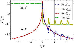
Figure 8: Correlation function $J^{>}$: comparison of analytic approximation $J^{>}_{\rm ana}$ given by Eq. (56) and numerical results $J^{>}_{\rm num}$ for $\omega_{c}\tau=25$.

IV Strong interaction: analytical solution

As shown in Sec. III, the considered model of a MZI with inside-only interaction can be exactly solved by the non-equilibrium functional bosonization method. The result is expressed in terms of single-particle objects: determinants and resolvents of Fredholm operators. While it is not too difficult to evaluate such quantities numerically, it would be highly advantageous to have a fully analytical solution of the problem. Such a solution will be obtained in the present section for the regime of strong interaction, $E_{c}\tau\gg 1$. This solution will allow us to understand much better the physics of the problem, including the formation of the visibility oscillations (taking a form of “lobes” in certain situations as discussed above) and their decay with voltage. Further, while determining the exact solution, we will establish a deep connection of the present problem with that of non-equilibrium Luttinger liquid and, more generally, with a broader class of non-equilibrium many-body problems.

As we have demonstrated in Sec. III, the “counting phase” in the strong-interaction regime, $E_{c}\tau\gg 1$, is reduced to the “window” function on the interval $[\bar{t},\bar{t}+\tau]$. We will show in Sec. IV.1 that under this condition the interference current can be represented in terms of singular Fredholm determinants generalizing Toeplitz determinants with Fisher-Hartwig singularities. Using asymptotic properties of such determinants (Sec. IV.2), we further derive the high-voltage form of the AB contribution to the current (Sec. IV.3). The result is Eq. (9) which has been already discussed in detail in Sec. II.2.

IV.1 Reduction to a single-channel problem

In Sec. III.2 we have expressed the interference current in terms of the operator ${\cal D}$ and the non-equilibrium density matrix $\tilde{f}$ which, in addition to being the matrices in the time space, have also a nontrivial channel structure: for given times $t_{1},t_{2}$ they are matrices from $\mathbb{C}^{2\times 2}$. (Since all the relevant non-equilibrium physics arising due to scattering at QPCs concerns only the outer channels, we focus on these two channels. In what follows we consider projections of all operators, such as $\hat{\vartheta}^{q}$, $\hat{f}$, onto the two outer channels; thus they retain the smaller $2\times 2$-channel structure.) The double index structure (times and channels) very seriously complicates the computation of the determinant and finding the inverse of ${\cal D}$. In this section, using the Riemann-Hilbert technique, we reduce the matrix determinant and resolvent to a product of certain single-channel determinants. We show that the corresponding operators belong to the class of singular Fredholm operators that may be considered as a generalization of Toeplitz matrices with Fisher-Hartwig singularities. The reduction to a single channel problem will allow us to calculate analytically the current in MZI, see Sec. IV.2 and IV.3 below.

IV.1.1 Heuristic argument: Relation to full counting statistics

Before presenting a rigorous derivation of the reduction formula, we will put forward a more heuristic argument in its favor. This argument is based on a connection between the fermion action ${\cal A}_{\rm ferm}$ and the theory of the full counting statistics (FCS). Consider the cumulant generating function (CGF) for the statistics of $N_{\pm}$, the numbers of non-interacting electrons which tunnel through the QPC1 during the time interval $[\bar{t},\bar{t}+\tau]$ into the upper/lower arm, resp.

$$\chi_{\tau}(\lambda_{+},\lambda_{-})=\langle e^{i\lambda_{+}\hat{N}_{+}+i\lambda_{-}\hat{N}_{-}}\rangle$$ (59)

with corresponding “counting fields” $\lambda_{\pm}$. The brackets here mean a quantum-statistical average. It is known Levitov et al. (1996) that this CGF can be represented as a functional determinant,

$$\chi_{\tau}(\lambda_{+},\lambda_{-})={\rm Det}\left[{\mathds{1}}-\hat{f}+s_{1}^{\dagger}e^{i\hat{\lambda}}s_{1}\hat{f}\right],$$ (60)

where $\hat{f}={\rm diag}(f_{+},f_{-})$ is the incoming distribution matrix of the 1st (outer) channel of the MZI. The counting fields here are assumed to have a time-dependence given by the “window” function (58). In this way the measuring time is encoded in the above formula. Let $f_{-}^{1}$ is set to the equilibrium Fermi distribution, and $f_{+}^{1}$ is the Fermi distribution with the chemical potential $eV$. Asymptotically, at $eV\tau\gg 1$, and dropping the equilibrium contribution $i(\lambda_{+}+\lambda_{-})(\tau/2\pi)\int_{-\infty}^{0}d\epsilon$ (which is infinite because of the chirality), we obtain

$$\ln\left[\chi_{\tau}(\lambda_{+},\lambda_{-})\right]\simeq\frac{eV\tau}{2\pi}\ln\left[R_{1}e^{i\lambda_{+}}+T_{1}e^{i\lambda_{-}}\right].$$ (61)

By comparing the Eqs. (60) and (35) we conclude that in the limit $E_{c}\tau\gg 1$

$$e^{i{\cal A}_{\rm ferm}}={\rm Det}\,{\cal D}=\chi_{\tau}\left(2\bar{\vartheta}_{+},2\bar{\vartheta}_{-}\right).$$ (62)

Because of this relation to the theory of FCS we will frequently refer to the matrix ${\cal D}$ as the “counting operator”. In the presence of scattering at QPC1 this operator possesses a $2\times 2$-matrix structure in the channel space. Consider further a single chiral channel with some (in general, non-equilibrium) distribution function $f$ and the phase $\delta(t)=w_{\bar{t},\tau}(t)\delta$. Then the generating function $\Delta_{\tau}[\delta,f]=\langle e^{i\delta\hat{N}}\rangle$ of the number $N$ of electrons passing by some observation point during the time interval $[\bar{t},\bar{t}+\tau]$ is given by the determinant of a “scalar” counting operator of the kind

$$\Delta_{\tau}[\delta,f]={\rm Det}\left[{\mathds{1}}+(e^{i\delta}-1)f\right].$$ (63)

We now argue that the determinant of the matrix counting operator ${\cal D}$, evaluated on the Fermi-like distribution functions (which is the case of reflectionless QPC0 with $R_{0}=1$) can be factorized into a product of “scalar” determinants of the type (63).

Let us take a closer look on the random numbers $\hat{N}_{\pm}$ in the CGF given by Eq. (59). In the strongly non-equilibrium situation which we consider, i.e. when voltage dominates over the temperature, they should be significantly negatively correlated (due to partition at QPC1), while their sum, $\hat{N}=\hat{N}_{+}+\hat{N}_{-}$ should be much less sensitive to scattering and will only weakly fluctuate around $\langle\hat{N}\rangle=eV\tau/(2\pi)+N_{0}$ with $N_{0}$ being some equilibrium contribution. (At the strictly zero temperature and long time limit $\hat{N}$ does not fluctuate at all.) We thus expect that $\hat{N}$ and $\hat{N}_{+}$ are only weakly correlated. Taking further into account that $\bar{\vartheta}_{+}=-\bar{\vartheta}_{-}$, we obtain

$$\chi_{\tau}\left(2\bar{\vartheta}_{+},2\bar{\vartheta}_{-}\right)=\langle e^{2i\vartheta_{+}^{q}\hat{N}_{+}+2i\vartheta_{-}^{q}\hat{N}_{-}}\rangle=$$

$$\langle e^{4i\vartheta^{q}_{+}\hat{N}_{+}-2i\vartheta^{q}_{+}\hat{N}}\rangle\simeq\langle e^{4i\vartheta^{q}_{+}\hat{N}_{+}}\rangle\langle e^{-2i\vartheta^{q}_{+}\hat{N}}\rangle.$$ (64)

This representation maps our 2-channel problem to three single-channel ones. The term $\langle e^{4i\bar{\vartheta}_{+}\hat{N}_{+}}\rangle$ requires us to count the charge in a single channel of the upper arm. It is characterized by the distribution function

$$f_{++}(\epsilon)=R_{1}\theta(eV-\epsilon)+T_{1}\theta(-\epsilon)$$

established by the QPC1, thus we conclude that

$$\langle e^{4i\bar{\vartheta}_{+}\hat{N}_{+}}\rangle=\Delta_{\tau}[4\bar{\vartheta}_{+},f_{++}].$$ (65)

The second term, $\langle e^{-2i\bar{\vartheta}_{+}\hat{N}}\rangle=\langle e^{-2i\bar{\vartheta}_{+}(\hat{N}_{+}+\hat{N}_{-})}\rangle$, counts the total charge in both arms. In view of charge conservation this total charge can be also measured in the incoming channels the contribution of which are uncorrelated. The corresponding distribution functions are $f_{+}(\epsilon)=\theta(eV-\epsilon)$ and $f_{-}(\epsilon)=\theta(-\epsilon)$. Therefore, we get

$$\langle e^{-2i\bar{\vartheta}_{+}\hat{N}}\rangle=\Delta_{\tau}[-2\bar{\vartheta}_{+},f_{+}]\,\Delta_{\tau}[-2\bar{\vartheta}_{+},f_{-}].$$ (66)

Combining the relations (64-66) we arrive at the following result:

$$\chi_{\tau}(2\bar{\vartheta}_{+},-2\bar{\vartheta}_{+}) =\Delta_{\tau}[4\bar{\vartheta}_{+},f_{++}]$$

$$\times\Delta_{\tau}[-2\bar{\vartheta}_{+},f_{+}]\,\Delta_{\tau}[-2\bar{\vartheta}_{+},f_{-}].$$ (67)

Finally, we complete the argument by using Eq. (62), which yields the desired decomposition of the matrix determinant ${\rm Det}\,{\cal D}$ into a product of scalar determinants:

$${\rm Det}\,{\cal D} =\Delta_{\tau}[4\bar{\vartheta}_{+},f_{++}]$$

$$\times\Delta_{\tau}[-2\bar{\vartheta}_{+},f_{+}]\,\Delta_{\tau}[-2\bar{\vartheta}_{+},f_{-}].$$ (68)

The following remark is of order here. The equalities between the determinants arising in our context and in the context of the counting statistics are, strictly speaking, valid for not too large values of the counting phase. For larger phases the counting statistics determinants show singularities and switch to another Riemannian sheet, while our determinants behave analytically, see Refs. Gutman et al., 2010b, c for an extended discussion. Physically, this is due to the fact that the counting statistics “knows” about the charge quantization, whereas for our problem the charge quantization is of no relevance. This remark does not affect the validity of the final result (68), since both sides of this equation are analytic functions of the phases.

IV.1.2 Rigorous proof: Riemann-Hilbert method

We are now going to prove Eq. (68) rigorously by analyzing the associated Riemann-Hilbert (RH) problem. We consider the function

$$Y(t)=\exp\left[\frac{\bar{\vartheta}_{+}}{\pi}\ln\frac{t-\bar{t}}{t-\bar{t}-\tau}\right],$$ (69)

which is analytic and non-zero in the complex plane $t\in{\mathbb{C}}$, except for the interval of real times $[\bar{t},\bar{t}+\tau]$. It has the property $Y(t)\to 1$ at $|t|\to\infty$. Next we define the functions $Y_{\pm}(t)=Y(t\pm i0)$ on the real axis, $t\in{\mathbb{R}}$. They solve the (scalar) RH problem $Y^{-1}_{-}(t)Y_{+}(t)=e^{-2i\vartheta_{+}^{q}(t)}$, where $\vartheta_{+}^{q}(t)=\bar{\vartheta}_{+}w_{\bar{t},\tau}(t)$. The functions $Y_{\pm}(t)$ obey important identities,

$$f_{0}^{<}\,Y_{-}\,f_{0}^{<} = f_{0}^{<}\,Y_{-},\quad f_{0}^{>}\,Y_{-}\,f_{0}^{>}=Y_{-}\,f_{0}^{>},$$

$$f_{0}^{<}\,Y_{+}\,f_{0}^{<} = Y_{+}\,f_{0}^{<},\quad f_{0}^{>}\,Y_{+}\,f_{0}^{>}=f_{0}^{>}\,Y_{+},$$ (70)

where the convolution in time on the left-hand side of these relations is implied and we set $f_{0}^{<}(t)\equiv f_{0}(t)$ and $f_{0}^{>}(t)=\delta(t)-f_{0}(t)=f_{0}(-t)$. As an example, the first relation in Eq. (70) reads in explicit notations as follows:

$$\int dt\frac{i/2\pi}{t_{1}-t+i0}Y_{-}(t)\frac{i/2\pi}{t-t_{2}+i0}=\frac{i/2\pi}{t_{1}-t_{2}+i0}Y_{-}(t_{2}).$$ (71)

Due to analytical properties of $Y_{-}(t)$ this integral is defined by the residue at $t=t_{2}-i0$ in the lower half-plane. We also note that in the energy domain at zero temperature, $f^{<}_{0}$ is the projector on occupied states, whereas $f_{0}^{>}$ projects on unoccupied states. Therefore, we have $(f_{0}^{>})^{2}=f_{0}^{>}$, $(f_{0}^{<})^{2}=f_{0}^{<}$, $f_{0}^{>}f_{0}^{<}=0=f_{0}^{<}f_{0}^{>}$, and $f_{0}^{<}+f_{0}^{>}=1$. The same relations hold in the time domain as well, where the product of two operators is understood in the sense of convolution. Using the basic identities (70) one derives another two useful relations,

$$f_{0}^{<}\,Y_{-}\,f_{0}^{>}=0,\quad f_{0}^{>}\,Y_{+}\,f_{0}^{<}=0.$$ (72)

Let us now turn to the analysis of the counting operator ${\cal D}$ defined by Eq. (35). We introduce the gauge matrix $\Lambda={\rm diag}(e^{-ieV_{+}t},e^{-ieV_{-}t})$ comprising voltages $V_{\pm}$ applied to the outer channel in the upper/lower arms. By using these gauge factors one rewrites ${\cal D}$ as

$${\cal D}=\Lambda\left(f_{0}^{>}+\Lambda^{-1}s_{1}^{\dagger}e^{2i\hat{\vartheta}^{q}}s_{1}\Lambda\,f_{0}^{<}\right)\Lambda^{-1}.$$ (73)

With the use of solution to the RH problem we have the identity ($\vartheta_{+}^{q}=-\vartheta_{-}^{q}$)

$$\Lambda^{-1}s_{1}^{\dagger}\begin{pmatrix}e^{2i\vartheta^{q}_{+}}&0\\ 0&e^{2i\vartheta^{q}_{-}}\end{pmatrix}s_{1}\Lambda$$

$$\hskip 28.45274pt=\Lambda^{-1}s_{1}^{\dagger}\begin{pmatrix}e^{4i\vartheta^{q}_{+}}&0\\ 0&{\mathds{1}}\end{pmatrix}s_{1}\Lambda\ Y_{-}^{-1}Y_{+}.$$ (74)

Bearing in mind that $Y_{-}^{-1}$ is a local in time operator without matrix structure in the channel space, one can commute it to the left of Eq. (74). In this way we find

$${\mathcal{D}}=\Lambda Y_{-}^{-1}\Bigl{[}Y_{-}f_{0}^{>}+\Lambda^{-1}s_{1}^{\dagger}\begin{pmatrix}e^{4i\vartheta^{q}_{+}}&0\\ 0&{\mathds{1}}\end{pmatrix}s_{1}\Lambda Y_{+}f_{0}^{<}\Bigr{]}\Lambda^{-1}.$$ (75)

To proceed further we apply the unitary transformation, $\tilde{\cal D}=s_{1}{\cal D}s_{1}^{\dagger}$, and factorize the operator $\tilde{\cal D}$ into a product of scalar counting operators. This is possible by virtue of the identity

$$\left(f_{0}^{>}+Af_{0}^{<}\right)\,\left(Y_{-}f_{0}^{>}+Y_{+}f_{0}^{<}\right)=Y_{-}f_{0}^{>}+AY_{+}f_{0}^{<},$$ (76)

which is valid for a local in time $2\times 2$ matrix $A(t)$. As one can check, the above relation follows directly from the projector properties, given by Eqs. (70) and (72). By setting

$$A=\Lambda^{-1}s_{1}^{\dagger}\begin{pmatrix}e^{4i\vartheta^{q}_{+}}&0\\ 0&{\mathds{1}}\end{pmatrix}s_{1}\Lambda,$$ (77)

we obtain

$$\tilde{\cal D} =Y_{-}^{-1}s_{1}\Lambda\left[f_{0}^{>}+\Lambda^{-1}s_{1}^{\dagger}\begin{pmatrix}e^{4i\vartheta^{q}_{+}}&0\\ 0&{\mathds{1}}\end{pmatrix}s_{1}\Lambda f_{0}^{<}\right]\Lambda^{-1}s_{1}^{\dagger}$$

$$\times s_{1}\Lambda\left[Y_{-}f_{0}^{>}+Y_{+}f_{0}^{<}\right]\Lambda^{-1}s_{1}^{\dagger}.$$ (78)

If one further introduces operators

$${\cal D}_{\ast} \equiv{\mathds{1}}+\begin{pmatrix}e^{4i\vartheta^{q}_{+}}-{\mathds{1}}&0\\ 0&0\end{pmatrix}\tilde{f},$$ (79)

$$\mathcal{D}_{0} \equiv{\mathds{1}}+\left(e^{-2i\vartheta^{q}_{+}}-{\mathds{1}}\right)\hat{f},$$ (80)

where

$$\tilde{f}=s_{1}\hat{f}s_{1}^{\dagger}=\begin{pmatrix}f_{++}&f_{+-}\\ f_{-+}&f_{--}\end{pmatrix}$$

is the non-equilibrium density matrix in the MZI cell. Explicitly, we have $f_{++}=R_{1}f_{+}^{1}+T_{1}f_{-}^{1}$ and $f_{+-}=i(R_{1}T_{1})^{1/2}(f_{+}^{1}-f_{-}^{1})$. Then $\tilde{\cal D}$ is equivalently rewritten as

$$\tilde{\cal D}=Y_{-}^{-1}\mathcal{D}_{\ast}s_{1}Y_{-}\mathcal{D}_{0}s_{1}^{\dagger}.$$ (81)

To obtain the operator $\mathcal{D}_{0}$ we have used here once again the solution of the RH problem. We hence conclude that

$${\rm Det}\,\tilde{\cal D}={\rm Det}\,{\cal D}_{*}\,{\rm Det}\,{\cal D}_{0}.$$ (82)

It is now straightforward to evaluate two determinants appearing on the right-hand side of this relation. In the case of matrix ${\cal D}_{*}$ we obtain

$${\cal D}_{*}=\begin{pmatrix}\mathcal{D}_{\ast\ast}&\left(e^{4i\vartheta^{q}_{+}}-{\mathds{1}}\right)f_{+-}\\ 0&{\mathds{1}}\end{pmatrix},$$ (83)

where the scalar (in the channel space) counting operator

$$\mathcal{D}_{\ast\ast}\equiv{\mathds{1}}+\left(e^{4i\vartheta^{q}_{+}}-{\mathds{1}}\right)f_{++}$$ (84)

is expressed solely in terms of the upper diagonal block of the density matrix $f_{++}$, which, obviously, has the meaning of the non-equilibrium distribution function in the upper arm of the MZI. As the result,

$${\rm Det}\,{\cal D}_{*}=\Delta_{\tau}[4\bar{\vartheta}_{+},f_{++}].$$ (85)

In the case of matrix ${\cal D}_{0}$ the incoming density matrix $\hat{f}$ is diagonal in the channel basis, that yields

$${\rm Det}\,{\cal D}_{0}=\Delta_{\tau}[-2\bar{\vartheta}_{+},f_{+}]\,\Delta_{\tau}[-2\bar{\vartheta}_{+},f_{-}].$$ (86)

Combining together Eqs. (82), (85), and (86), we obtain the relation (68). The proof of this formula is thus completed.

IV.1.3 Inversion of the matrix counting operator

In the preceding subsection we have proven that the determinant ${\rm Det}\,\tilde{\cal D}$ (or, equivalently, the fermion action ${\cal A}_{\rm ferm}$) can be expressed in terms of determinants of single-channel (scalar) operators. For the evaluation of the interference current one also needs to consider off-diagonal matrix elements ($\mu=-\kappa$) $\langle\mu|\tilde{f}\,\tilde{\cal D}^{-1}(\bar{t},\bar{t})|\kappa\rangle$, see Eq. (43). The goal of this subsection is to show that, similar to the action, the above matrix elements can be also expressed via the scalar counting operator ${\cal D}_{**}$, given by Eq. (84).

According to Eq. (81), the inverse of $\tilde{\cal D}$ can be written as

$$\tilde{\cal D}^{-1}=s_{1}\mathcal{D}_{0}^{-1}Y_{-}^{-1}s_{1}^{\dagger}\mathcal{D}_{\ast}^{-1}Y_{-}.$$ (87)

Making use of the solution to RH problem we then represent the counting operator (80) in the form

$$\mathcal{D}_{0}=\Lambda Y_{-}^{-1}\left(Y_{-}f_{0}^{>}+Y_{+}f_{0}^{<}\right)\Lambda^{-1}.$$ (88)

The basic relation of the RH method,

$$\left(Y_{-}f_{0}^{>}+Y_{+}f_{0}^{<}\right)^{-1}=Y_{-}^{-1}f_{0}^{>}+Y_{+}^{-1}f_{0}^{<},$$ (89)

easily gives the inverse of ${\cal D}_{0}$ (one can check the former identity by multiplying two operators to get the unity, employing for that relations (70) and (72)). The inverse of $\tilde{\cal D}$ then reads

$$\tilde{\cal D}^{-1}=s_{1}\hat{\Lambda}\left[Y_{-}^{-1}f_{0}^{>}+Y_{+}^{-1}f_{0}^{<}\right]\hat{\Lambda}^{-1}s_{1}^{\dagger}\mathcal{D}_{\ast}^{-1}Y_{-},$$ (90)

and the subsequent convolution with the MZI’s density matrix $\tilde{f}$ yields

$$\tilde{f}\tilde{\cal D}^{-1}=s_{1}\hat{\Lambda}f_{0}\hat{\Lambda}^{-1}s_{1}^{\dagger}\tilde{\cal D}^{-1}=Y_{+}^{-1}\tilde{f}\mathcal{D}_{\ast}^{-1}Y_{-}$$ (91)

The required $(\mu\bar{t},\kappa\bar{t})$ matrix element of this operator then takes the form

$$\left\langle\mu\right\rvert\tilde{f}\tilde{\cal D}^{-1}(\bar{t},\bar{t})\left\lvert\kappa\right\rangle =\left(Y_{+}^{-1}Y_{-}\right)(\bar{t})\ \left\langle\mu\right\rvert\tilde{f}\mathcal{D}_{\ast}^{-1}(\bar{t},\bar{t})\left\lvert\kappa\right\rangle$$

$$=e^{2i\bar{\vartheta}_{+}}\left\langle\mu\right\rvert\tilde{f}\mathcal{D}_{\ast}^{-1}(\bar{t},\bar{t})\left\lvert\kappa\right\rangle.$$ (92)

The inversion of the operator $\mathcal{D}_{\ast}$ appearing here is not exactly trivial, but it is simplified a lot due to its triangular structure (83) in the channel space. Note that the relation $\mathcal{D}_{\ast\ast}(t_{1},t_{2})=\delta(t_{1}-t_{2})$ for $t_{1}\notin[\bar{t},\bar{t}+\tau]$ implies the same for the inverse, $\mathcal{D}^{-1}_{\ast\ast}(t_{1},t_{2})=\delta(t_{1}-t_{2})$ for $t_{1}\notin[\bar{t},\bar{t}+\tau]$ (this can be seen by employing the block matrix representation or using the reformulation in terms of the Riemann-Hilbert problem). One therefore obtains

$$\left\langle-\right\rvert\tilde{f}\mathcal{D}_{\ast}^{-1}(\bar{t},\bar{t})\left\lvert+\right\rangle =f_{-+}\mathcal{D}_{\ast\ast}^{-1}(\bar{t},\bar{t})=f_{-+}w_{\bar{t},\tau}\ \mathcal{D}_{\ast\ast}^{-1}(\bar{t},\bar{t}),$$ (93)

and the analogous relation for the conjugated matrix element,

$$\left\langle+\right\rvert\tilde{f}\mathcal{D}_{\ast}^{-1}(\bar{t},\bar{t})\left\lvert-\right\rangle =\left[f_{+-}-f_{++}\mathcal{D}^{-1}_{\ast\ast}\left(e^{4i\vartheta_{+}^{q}}-{\mathds{1}}\right)f_{+-}\right]_{\bar{t},\bar{t}}$$

$$=\mathcal{D}_{\ast\ast}^{-1}w_{\bar{t},\tau}\ f_{+-}(\bar{t},\bar{t}).$$ (94)

It is worth pointing out that the instanton phases $\bar{\vartheta}_{\eta}=\pm\eta\pi/\nu$ in Eqs. (93) and (94) have opposite signs (and hence $\mathcal{D}_{\ast}$ and $\mathcal{D}_{\ast\ast}$ differ between these two equations). Since under complex conjugation $f_{\eta}(t)^{\ast}=f_{\eta}(-t)$, these two matrix elements are indeed complex conjugates of each other. Relations (93) and (94) are the final result of this subsection and will be used below in Secs. IV and V for evaluation of the interference current.

IV.2 Toeplitz matrices and their generalizations

In this subsection we relate the current and the action to the theory of Toeplitz matrices. We review key results on the large-$N$ asymptotic behavior of Toeplitz determinants with “Fisher-Hartwig singularities” and of a more general class of singular Fredholm determinants. These results will be then used to calculate the determinant and the inverse of the operator ${\cal D}_{**}$, which will serve as the basis for the calculation of the AB conductance made in Sec. IV.3.

IV.2.1 From integral operators to Toeplitz matrices

We relate first the fermion action ${\cal A}_{\rm ferm}$ to the theory of Toeplitz matrices. As we have shown in the previous section, the action is expressed in terms of single-particle counting operators, see Eq. (68).

The linearized single-particle spectrum used in our 1D model lacks upper and lower band edges. Thus, a definition of the determinant of such operators requires an ultra-violet (UV) regularization. One possible way to implement the regularization is a discretization of the time coordinate $t$ in steps $\Delta t=\pi/\Lambda$, which amounts to the introduction of an UV cutoff $\Lambda$ and restriction of energies to the range $[-\Lambda,\Lambda]$. In this regularization procedure operators with kernels such as $\mathcal{D}_{\ast\ast}(t_{1},t_{2})$, cf. (84), are turned into (in general, infinite) matrices with discrete time indices.

In the limit of strong interaction the phase $\vartheta^{q}_{\eta}=\bar{\vartheta}_{\eta}w_{\bar{t},\tau}$ is a piecewise constant function which vanishes outside the interval $[\bar{t},\bar{t}+\tau]$. Introducing the projector $P$ which acts on functions $\phi(t)$ by multiplication with a window function in time, $P\phi=\phi w_{\bar{t},\tau}$, and thus satisfies $P^{2}=P$, we can write

$${\rm Det}\,\mathcal{D}_{\ast\ast} ={\rm Det}\,\left[{\mathds{1}}+P\left(e^{4i\bar{\vartheta}_{+}}-1\right)f_{++}\right]$$

$$={\rm Det}\,\left[{\mathds{1}}+P\left(e^{4i\bar{\vartheta}_{+}}-1\right)f_{++}P\right].$$ (95)

The operator $g_{\ast\ast}\equiv{\mathds{1}}+P\left(e^{4i\bar{\vartheta}_{+}}-1\right)f_{++}P$ has a block structure, namely

$$g_{\ast\ast}(t_{1},t_{2})=\left\{\begin{array}[]{ll}g(t_{1}-t_{2}),&t_{1},t_{2}\in[\bar{t},\bar{t}+\tau],\\ \delta(t_{1}-t_{2}),&{\rm otherwise},\end{array}\right.$$ (98)

where

$$g(t_{1}-t_{2})\equiv\delta(t_{1}-t_{2})+\left(e^{4i\bar{\vartheta}_{+}}-1\right)f_{++}(t_{1}-t_{2}).$$ (99)

The kernel of the operator $g_{\ast\ast}$ is nontrivial only if both $t_{1}$ and $t_{2}$ lie in the interval $[\bar{t},\bar{t}+\tau]$, in which case it depends solely on the difference $t_{1}-t_{2}$. The determinant of $g_{\ast\ast}$ will be given by the nontrivial block $g(t_{1}-t_{2})$. The UV regularization of $g$ as described above will give rise to a large $N\times N$-matrix $\left(g_{jk}\right)_{1\leq j,k\leq N}$, $N=\tau/\Delta t=\Lambda\tau/\pi$, whose elements depend on index differences, $g_{jk}=g_{j-k}$. The matrix $(g_{jk})$ of such type is known as a Toeplitz matrix.

Matrices of Toeplitz form are ubiquitous in mathematics and physics where they appear in a variety of contexts (see e.g. Fisher and Hartwig (1968); Krasovsky (2011) for summaries of applications). It was shown in Refs. Gutman et al., 2010b, c, 2011 that observables in a vast range of problems of 1D non-equilibrium interacting fermions (and bosons) can be expressed in terms of Toeplitz determinants $\Delta_{N}=\det\left(g_{i-j}\right)_{1\leq i,j\leq N}$.

The behavior of determinants of such matrices becomes particularly non-trivial when the corresponding symbol (essentially the Fourier transform of $g_{j-k}$, see Sec. IV.2 for more detail) has singular points known as Fisher-Hartwig singularities. In our case such singularities arise in view of discontinuities of the double-step distribution function $f_{++}$. In Refs. Gutman et al., 2011; Protopopov and Mirlin, 2011 the large-$N$ behavior of Toeplitz determinants with Fisher-Hartwig singularities has been established analytically and verified numerically. These results (“generalized Fisher-Hartwig conjecture”) go beyond the “standard” Fisher-Hartwig conjecture (proven in Ref. Deift et al., 2011) as they contain not only the leading term but also subleading power-law contributions that have different oscillatory factors. We will see below that taking into account such contributions will be crucial for obtaining the oscillatory dependence of visibility of MZI on voltage. A further generalization was achieved recently in Ref. Protopopov et al., 2012 where a broader class of singular Fredholm determinants (determined by two symbol functions that show multiple singularities in energy and coordinate spaces, respectively) was explored and corresponding asymptotics were found. Such determinants will arise below when we will invert the operator ${\cal D}_{**}$.

IV.2.2 Asymptotics of Toeplitz determinants

For the benefit of the reader we summarize here the relevant results on Toeplitz determinants.

A Toeplitz matrix $g_{jk}$ with $j,k=1,2,\ldots,N$ is defined by its symbol $g(z)$ as follows:

$$g_{jk}=g_{j-k}=\int_{-\pi}^{\pi}\!\frac{d\varphi}{2\pi}\,g(e^{i\varphi})e^{-i\varphi(j-k)}.$$ (100)

The determinant of such a matrix is called Toeplitz determinant. An important class of Toeplitz matrices (which is of relevance for our work and for various other non-equilibrium many-body problems) is generated by symbols with Fisher-Hartwig (FH) singularities,

$$g(z)=e^{V(z)}\prod_{j=0}^{m}\left\lvert z-z_{j}\right\rvert^{2\alpha_{j}}\ \gamma_{j}(z)\left(z/z_{j}\right)^{\beta_{j}}$$ (101)

where $V(z)$ is a smooth function, $m+1$ is a positive integer (number of singular points), $z_{j}\equiv e^{i\varphi_{j}}$, ${\rm Re}\,\alpha_{j}>-\frac{1}{2}$, $\beta_{j}\in\mathbb{C}$, and

$$\gamma_{j}(z)=\left\{\begin{array}[]{ll}e^{i\pi\beta_{j}},&-\pi<\arg z<\varphi_{j},\\ e^{-i\pi\beta_{j}},&\varphi_{j}<\arg z<\pi.\end{array}\right.$$ (104)

In the context of our work, only the case $\alpha_{j}=0$ (when the singularities of $f(z)$ are discontinuities) will be relevant, so that we consider it henceforth. The large-$N$ asymptotic behavior of the corresponding Toeplitz determinant $\Delta_{N}$ readsGutman et al. (2011); Protopopov and Mirlin (2011):

$$\Delta_{N}=e^{NV_{0}}\sum_{n_{0}+\ldots+n_{m}=0}\,\prod_{j=0}^{m}z_{j}^{n_{j}N}\ \left[N^{-\sum_{j=0}^{m}\beta_{j}^{2}}\ \prod_{0\leq j<k\leq m}\left\lvert z_{j}-z_{k}\right\rvert^{2\beta_{j}\beta_{k}}\ \prod_{j=0}^{m}G(1+\beta_{j})G(1-\beta_{j})\right]_{\beta_{j}\to\beta_{j}+n_{j}}(1+\ldots).$$ (105)

where $V_{0}=\int_{-\pi}^{\pi}\!\frac{d\varphi}{2\pi}\,V(e^{i\varphi})$ and $G$ is the Barnes G-function. The summation in Eq. (105) goes over a set of integers $n_{0}$, $n_{1}$, …, $n_{m}$ (whose sum is zero); we will see below that they can be understood as labeling branches of $\log g(z)$ in the intervals of continuity of the symbol. Each of these sets (“branches”) is characterized by a distinct factor $\prod_{j=0}^{m}z_{j}^{n_{j}N}$ that in our context will give rise to a distinct oscillatory exponent. Equation (105) presents explicitly the leading asymptotic behavior for each of the branches. There exist also subleading power-law corrections within each of the branches (i.e., corresponding to the same oscillatory exponent); they are abbreviated by $+\ldots$ in the last bracket. Such corrections will be of no importance for our consideration, and we discard them below.

We return now to determinants of the type (63) that arise in the course of the study of MZI. Here $f$ is some distribution function and $\delta(t)=\delta w_{[0,\tau]}(t)$ is a constant in the window of the duration $\tau$ and zero otherwise. We are interested in the large-$\tau$ asymptotic behavior of $\Delta_{\tau}[\delta,f]$. As discussed in Sec. IV.2.1, the UV regularization is implemented by using a high-energy cut-off $\Lambda$, so that the energy is restricted to the range $[-\Lambda,\Lambda]$ and the time is discretized, $t_{j}=j\Delta t=j\pi/\Lambda$. In energy representation, the operator of interest reads [cf. Eq. (99)]

$$\tilde{g}(\epsilon)=1+(e^{i\delta}-1)f(\epsilon).$$ (106)

This can be identified with a symbol $g(z)$ of a Toeplitz matrix, provided energy $\epsilon\in[-\Lambda,\Lambda]$ and angle $\varphi\in[-\pi,\pi]$ are related by rescaling: $\varphi=\epsilon\pi/\Lambda$. The introduction of a hard cutoff $\pm\Lambda$ and the above compactification of the energy axis will give rise to unphysical effects at this energy scale (since it will generate an unphysical discontinuity at $\varphi=\pm\pi$). These unphysical effect are eliminated by imposing “periodic boundary conditions” in energy domainGutman et al. (2011), which amounts to the following modification of the symbol: $\lim_{\epsilon\to-\Lambda}g(\epsilon)=\lim_{\epsilon\to\Lambda}g(\epsilon)$:

$$g(\epsilon)=e^{i\delta\epsilon/(2\Lambda)}\left[1+(e^{i\delta}-1)f(\epsilon)\right].$$ (107)

Here we have taken into account that $\lim_{\epsilon\to-\Lambda}f(\epsilon)=1$ and $\lim_{\epsilon\to\Lambda}f(\epsilon)=0$.

To be specific, let us consider explicitly two examples corresponding to two lowest values $m=0,1$ (i.e., one and two FH singularities.) First, we consider the equilibrium distribution function $f(\epsilon)=\theta(\mu-\epsilon)$. The symbol is

$$g(e^{i\varphi})=\left\{\begin{array}[]{ll}e^{i\delta\varphi/(2\pi)}e^{i\delta},&-\pi<\varphi<\pi\mu/\Lambda,\\ e^{i\delta\varphi/(2\pi)},&\pi\mu/\Lambda<\varphi<\pi,\end{array}\right.$$ (110)

which is of the form (101) with $m=0$, $\alpha_{0}=0$, $\beta_{0}=\delta/(2\pi)$, $z_{0}=e^{i\pi\mu/\Lambda}$, and $V_{0}=i\delta(1+\mu/\Lambda)/2$. According to Eq. (105) in the large-$N$ limit the $\det(g_{j-k})$ asymptotically behaves as

$$\Delta[\delta,f_{\rm single}] =\exp\left[{i\frac{\delta}{2\pi}(\Lambda+\mu)\tau}\right]\ \left(\frac{\Lambda\tau}{\pi}\right)^{-\left(\frac{\delta}{2\pi}\right)^{2}}$$

$$\times G(1-\frac{\delta}{2\pi})\,G(1+\frac{\delta}{2\pi}).$$ (111)

Next, we consider a double-step distribution function $f(\epsilon)=(1-a)\,\theta(\mu_{0}-\epsilon)+a\,\theta(\mu_{1}-\epsilon)$, where we assumed that $\mu_{0}<\mu_{1}$. In this case the symbol reads

$$g(e^{i\varphi}) =\left\{\begin{array}[]{ll}e^{i\delta\varphi/(2\pi)}e^{i\delta},&-\pi<\varphi<\frac{\pi\mu_{0}}{\Lambda},\\ e^{i\delta\varphi/(2\pi)}\left[1+(e^{i\delta}-1)a\right],&\frac{\pi\mu_{0}}{\Lambda}<\varphi<\frac{\pi\mu_{1}}{\Lambda},\\ e^{i\delta\varphi/(2\pi)},&\frac{\pi\mu_{1}}{\Lambda}<\varphi<\pi.\end{array}\right.$$ (115)

Hence, the symbol has two FH singularities $z_{j}=e^{i\pi\mu_{j}/\Lambda}$, $j=0,1$, with

$$e^{-2\pi i\beta_{0}}=\frac{1+(e^{i\delta}-1)a}{e^{i\delta}},\quad e^{-2\pi i\beta_{1}}=\frac{1}{1+(e^{i\delta}-1)a}.$$ (116)

We choose

$$\beta_{1}=-\frac{i}{2\pi}\ln\left[1+(e^{i\delta}-1)a\right],\quad\beta_{0}=\frac{\delta}{2\pi}-\beta_{1}.$$ (117)

It is easy to see that the symbol has the form (101) with $m=1$, $\alpha_{j}=0$, and

$$V(z)=V_{0}=i\delta/2+i\delta\frac{\mu_{0}}{2\Lambda}+ieV\frac{\pi}{\Lambda}\beta_{1}$$ (118)

where we introduced $eV=\mu_{1}-\mu_{0}$. According to (105) the asymptotic behavior of the Toeplitz determinant $\det\left(g_{j-k}\right)$ is given by

$$\Delta[\delta,f_{\rm double}]=\exp\left[i\frac{\delta}{2\pi}(\Lambda+\mu_{0})\tau+\frac{eV\tau}{2\pi}\ln\left[1+(e^{i\delta}-1)a\right]\right]\,\sum_{n=-\infty}^{\infty}e^{-ieV\tau n}\ \left(\frac{\Lambda\tau}{\pi}\right)^{-(\beta_{0}+n)^{2}-(\beta_{1}-n)^{2}}\\ \times\left(\frac{\pi eV}{\Lambda}\right)^{2(\beta_{0}+n)(\beta_{1}-n)}\,G(1+\beta_{0}+n)G(1-\beta_{0}-n)G(1+\beta_{1}-n)G(1-\beta_{1}+n).$$ (119)

In order to identify in the sum over $n$ the leading contributions in the long-$\tau$ regime, we consider the exponent

$${\rm Re}\left[-(\beta_{0}+n)^{2}-(\beta_{1}-n)^{2}\right]=-2\left(n-n^{\ast}\right)^{2}+{\rm const},$$ (120)

where

$$n^{\ast} = \frac{1}{2}{\rm Re}(\beta_{1}-\beta_{0})$$ (121)

$$= {1\over{2\pi}}\mathrm{Im}\,\ln\left[(1-a)+ae^{i\delta}\right]-\frac{\delta}{4\pi}.$$

Note also that the sum of voltage and time exponents, $\left[-(\beta_{0}+n)^{2}-(\beta_{1}-n)^{2}\right]-\left[2(\beta_{0}+n)(\beta_{1}-n)\right]=-(\beta_{0}+\beta_{1})^{2}$ is independent of $n$. Thus, terms dominant for $\Lambda\tau\gg 1$ are also leading for large voltages, $eV\tau\gg 1$. For the analysis of the optimal value $n^{\ast}$, we make the decomposition $\delta=2\pi M+\delta^{\prime}$ with $M\in\mathbb{Z}$ and $\lvert\delta^{\prime}\rvert<\pi$. One can show that the phase

$$\delta^{\prime\prime}\equiv\mathrm{Im}\,\ln\left[(1-a)+ae^{i\delta}\right]$$ (122)

has the same sign as $\delta^{\prime}$ and satisfies $\lvert\delta^{\prime\prime}\rvert\leq\lvert\delta^{\prime}\rvert$. Then the optimal $n^{*}$ becomes

$$n^{\ast}=-\frac{M}{2}-\frac{\delta^{\prime}-2\delta^{\prime\prime}}{4\pi},\quad\lvert n^{\ast}+M/2\rvert\leq 1/4.$$ (123)

We see that in the case of even $M$ there is a single contribution with $n=-M/2$ giving the most significant contribution to the asymptotic series; other contributions have substantially smaller (by real part) exponents. On the other hand, for odd $M$ one has to take into account two contributions with $n=-(M\pm 1)/2$. Indeed, if $a=1/2$ (and thus $\delta^{\prime\prime}=\delta^{\prime}/2$), then these two contributions come with equal exponents. When $a$ deviates from 1/2, the exponents become different but still may be very close.

It was shown in Ref. Protopopov et al., 2012 that these results can be genralized to a broader class of singular Fredholm determinants. Specifically, consider a matrix

$$g_{j,k}=\int_{-\Lambda}^{\Lambda}\!\frac{d\epsilon}{2\Lambda}\,e^{-i\epsilon\pi/\Lambda[j-k-\delta(t_{j})/(2\pi)]}\tilde{g}(t_{j},\epsilon)$$ (124)

with the symbol

$$\tilde{g}(t,\epsilon)\equiv 1+\left(e^{i\delta(t)}-1\right)f(\epsilon).$$ (125)

Here the notion of symbol has been generalized to include both time and energy dependence (through the function $\delta(t)$ and $f(\epsilon)$, respectively). Let us focus on the case when both the phase $\delta(t)$ and the distribution function $f(\epsilon)$ are piecewise constant functions with jumps at times $\tau_{1}<\tau_{2}<\ldots<\tau_{N_{\tau}}$ and energies $\mu_{1}<\mu_{2}<\ldots<\mu_{N_{\mu}}$, respectively. They satisfy the boundary conditions $\delta(t)=0$ for $t\notin[\tau_{1},\tau_{N_{\tau}}]$, $f(\epsilon)=1$ for $\epsilon<\mu_{1}$, and $f(\epsilon)=0$ for $\epsilon>\mu_{N_{\mu}}$. The UV cutoff and the periodic boundary conditions in energy domain can be implemented as before. The discontinuity points define a grid which subdivides the time-energy plane in domains with different values of the symbol. The domains can be labeled by the time indices $j\in\{0,\ldots,N_{\tau}\}$, and energy indices $k\in\{0,\ldots,N_{\mu}\}$. One associates with this set of domains a set of number $c_{jk}$,

$$c_{jk}\equiv\frac{1}{2\pi i}\ln\tilde{g}(\tau_{j}+0,\mu_{k}+0)+n_{jk},$$ (126)

$$c_{j0}\equiv\delta(t_{j}+0)/(2\pi),\quad c_{0k}=c_{N_{\tau},k}=c_{j,N_{\mu}}=0.$$ (127)

where $\{n_{jk}\}$ is an arbitrary set of integers. Further, a matrix $\beta_{jk}$ with a time index $j\in\{1,\ldots,N_{\tau}\}$ and energy index $k\in\{1,\ldots,N_{\mu}\}$ is introduced according to

$$\beta_{jk}\equiv c_{j,k-1}-c_{j,k}+c_{j-1,k}-c_{j-1,k-1},$$ (128)

Physically, each entry of this matrix corresponds to a crossing point of one energy-space and one time-space singularity. In terms of this matrix, a set of time ($p_{jl}$) and energy ($q_{km}$) exponents is defined as follows:

$$p_{jl}\equiv\sum_{m^{\prime}=1}^{N_{\mu}}\beta_{jm^{\prime}}\beta_{lm^{\prime}},\quad q_{km}\equiv\sum_{l^{\prime}=1}^{N_{t}}\beta_{l^{\prime}k}\beta_{l^{\prime}m}.$$ (129)

One should keep in mind that $c_{jk}$ and thus $\beta_{jk}$, $p_{jl}$, and $q_{km}$ depend on the set of integers $n_{jk}$. In Eq. (126) the logarithm $\ln\tilde{g}$ is understood as evaluated at its principal branch, $\mathrm{Im}\,\ln\tilde{g}\in(-\pi,\pi]$. The summation over integers $n_{jk}$ hence amounts to summing over different branches of the logarithms.

We are now ready to state the result. For large time- and energy differences, $\lvert(\tau_{j}-\tau_{l})(\mu_{k}-\mu_{m})\rvert\gg 1$ ($j\neq l$, $k\neq m$), the asymptotic behavior of $\det(g_{j,k})$ is given byProtopopov et al. (2012)

$$\Delta[\delta(t),f(\epsilon)]=\sum_{\{n_{jk}\}}\Gamma_{\{n_{jk}\}}\ \exp\left[i\sum_{1\leq j<N_{t}}\left(c_{j0}(\Lambda+\mu_{1})+\sum_{1\leq k<N_{\mu}}c_{jk}\left(\mu_{k+1}-\mu_{k}\right)\right)(\tau_{j+1}-\tau_{j})\right]\\ \times\prod_{1\leq j<l<N_{t}}\prod_{1\leq k<m<N_{\mu}}\ \left\lvert\frac{\Lambda\left(\tau_{j}-\tau_{l}\right)}{\pi}\right\rvert^{p_{jl}}\left\lvert\frac{\pi\left(\mu_{k}-\mu_{m}\right)}{\Lambda}\right\rvert^{q_{km}}$$ (130)

with coefficients $\Gamma_{\{n_{jk}\}}$ that are independent on $\tau_{j}$ and $\mu_{k}$. It is not difficult to check that for the phase $\delta(t)$ proportional to a window function this formula agrees with the asymptotics (119) of the Toeplitz determinant. While a rigorous mathematical proof of the asymptotic formula (130) is still lacking, Ref. Protopopov et al., 2012 presented powerful analytical arguments in favor of its validity supported by strong evidence based on numerical evaluation of such determinants. We will use Eq. (130) below to get analytical results for the current through the MZI.

IV.2.3 Inversion of the single-channel counting matrix ${\cal D}_{**}$

As we have shown in Sec. IV.2, the interference current can be expressed in terms of the inverse of the single-channel counting operator ${\cal D}_{**}$. We show here that it is related to a generalized Toeplitz determinant, whose asymptotic behavior can be estimated on the basis of results presented above. To this end we consider the time discretized expression for the operator ${\cal D}_{**}$, given by Eq. (84), which has the symbol

$$g(\epsilon)=e^{2i\bar{\vartheta}_{+}\epsilon/\Lambda}\left[1+\left(e^{4i\bar{\vartheta}_{+}}-1\right)f_{++}(\epsilon)\right]$$ (131)

corresponding to the Toeplitz matrix,

$$g_{j-k} =\frac{i}{2\pi}\frac{1}{j-k-2\bar{\vartheta}_{+}/\pi}\left(e^{4i\bar{\vartheta}_{+}}-1\right)$$

$$\times\left[R_{1}e^{-i\pi U/\Lambda[j-k-2\bar{\vartheta}_{+}/\pi]}+T_{1}\right].$$ (132)

The inverse of matrix $g$ reads

$$\left(g^{-1}\right)_{jk}=(-1)^{j+k}\frac{\det g^{\sharp}(k,j)}{\det(g)},$$ (133)

where $g^{\sharp}(k,j)$ is the $(N-1)\times(N-1)$ matrix derived from $g$ by removing the $k$-th row and $j$-th column.

Since our primary interest is the matrix element $D_{**}^{-1}(\bar{t},t)$ with $\bar{t}<t<\bar{t}+\tau$, see Eq. (94), we concentrate specifically on the element $(g^{-1})_{1k}$, i.e. we put $j=1$. In this case one has

$$\left(g^{\sharp}(k,1)\right)_{lm} =\left\{\begin{array}[]{ll}g_{l,m+1},&1\leq l<k,\\ g_{l,m},&k\leq l\leq N-1\end{array}\right.$$ (136)

$$=\frac{i}{2\pi}\frac{1}{l-m-\frac{2}{\pi}\vartheta_{+}(t_{l};t_{k})}\left(e^{4i\vartheta_{+}(t_{l};t_{k})}-1\right)$$

$$\times\left[R_{1}e^{-i\pi U/\Lambda[j-k-\frac{2}{\pi}\vartheta_{+}(t_{l};t_{k})]}+T_{1}\right],$$ (137)

where we have introduced the time-dependent phase

$$\vartheta_{+}(t_{l};t_{k})=\left\{\begin{array}[]{ll}\bar{\vartheta}_{+}+\pi/2,&\bar{t}\leq t_{l}<t_{k},\\ \bar{\vartheta}_{+},&t_{k}\leq t_{l}<\tau+\bar{t}.\end{array}\right.$$ (140)

with $t_{l}=\bar{t}+(l-1)\Delta t$. In the continuous representation the phase $\vartheta_{+}(t,t_{k})$ is the piecewise function of time $t$. Taking into account Eqs. (132), (137) and the definition (124) one observes that the matrix $\left(g^{\sharp}(k,1)\right)_{lm}$ is the generalized Toeplitz matrix with the symbol (125) where the phase $\delta(t)=4\vartheta_{+}(t,t_{k})$. Its determinant can be dealt with by the use of results presented in the end of the previous subsection. Hence,

$$\left(g^{-1}\right)_{1k}=(-1)^{1+k}\frac{\Delta[4\vartheta_{+}(\bullet;t_{k}),f_{++}]}{\Delta[4\bar{\vartheta}_{+},f_{++}]}.$$ (141)

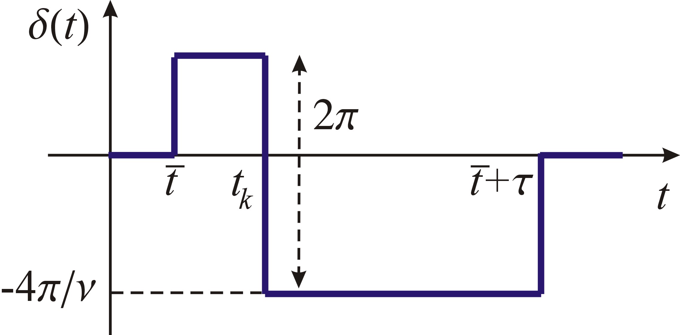
Figure 9: Phase $\delta(t)=4\vartheta_{+}(t;t_{k})$: on top of the “background phase” $4\vartheta_{+}^{q}(t)$ the $2\pi$-pulse accounts for the additional electron during the time interval $0<t<t_{k}$.

It is instructive to apply first the asymptotic relations (119) and (130) to invert the matrix $g_{j-k}$ in the limit $T_{1}\to 0$, when the alternative evaluation can be done via the Riemann-Hilbert method. Under this condition the operator ${\cal D}_{**}$ has the form

$$\left[{\cal D}_{**}\right]_{T_{1}\to 0}=\Lambda_{+}\left[f^{>}_{0}+e^{4i\vartheta_{+}^{q}}f_{0}^{<}\right]\Lambda_{+}^{-1}$$ (142)

with $\Lambda_{+}(t)=e^{-iV_{+}t}$. Therefore $\left[{\cal D}_{**}\right]_{T_{1}\to 0}^{-1}$ can be evaluated in the similar fashion as we have found the inverse of the counting operator ${\cal D}_{0}$ in Sec. IV.1.2. By introducing the function

$$\tilde{Y}(t)=\left(\frac{t-\bar{t}}{t-\bar{t}-\tau}\right)^{{2\bar{\vartheta}_{+}}/{\pi}},$$ (143)

which solves the RH problem $\tilde{Y}_{-}^{-1}\tilde{Y}_{+}=e^{-4i\vartheta_{+}^{q}}$, one further represents ${\cal D}_{**}$ in the equivalent form

$$\left[{\cal D}_{**}\right]_{T_{1}\to 0}=\Lambda_{+}\tilde{Y}_{-}\left[\tilde{Y}_{-}^{-1}f^{>}_{0}+\tilde{Y}_{+}^{-1}f_{0}^{<}\right]\Lambda_{+}^{-1}.$$ (144)

Using now the relation (89), we obtain

$$\left[\mathcal{D}_{\ast\ast}\right]_{T_{1}\to 0}^{-1}(\bar{t},t)=\tilde{Y}_{-}(\bar{t})\left[{\mathds{1}}+\left(e^{-4i\vartheta_{+}^{q}}-{\mathds{1}}\right)f_{+}\right]_{\bar{t},t}\tilde{Y}_{-}^{-1}(t).$$ (145)

Taking into account the explicit form of the solution of the RH problem (143), for times $t\in[\bar{t},\bar{t}+\tau]$ we eventually arrive at

$$\left[\mathcal{D}_{\ast\ast}\right]_{T_{1}\to 0}^{-1}(\bar{t},t) =-\frac{\Lambda}{\pi}\ e^{-2i\bar{\vartheta}_{+}}\sin(2\bar{\vartheta}_{+})\ e^{-ieV(\bar{t}-t)}$$

$$\times\left\lvert t-\bar{t}\right\rvert^{-2\bar{\vartheta}_{+}/\pi-1}\left\lvert\bar{t}+\tau-t\right\rvert^{2\bar{\vartheta}_{+}/\pi}$$

$$\times\tau^{-2\bar{\vartheta}_{+}/\pi}\Lambda^{-2\bar{\vartheta}_{+}/\pi-1}$$ (146)

where the regularization $\tilde{Y}_{-}(\bar{t})=\tilde{Y}_{-}(\bar{t}+\Lambda^{-1})$ was chosen.

Let us now demonstrate that the same result can be derived using the properties of the Toeplitz determinants. For $\mathcal{D}_{\ast\ast}^{-1}(\bar{t},t_{k})$ and thus $\left(g^{-1}\right)_{1k}$ one needs to consider the generalized Toeplitz problem with 3 jumps in time domain, $\tau_{1}=\bar{t}$, $\tau_{2}=t_{k}$, $\tau_{3}=\bar{t}+\tau$, and just 1 jump in energy domain $\mu_{1}=eV$. Further it is $c_{10}=2\bar{\vartheta}_{+}/\pi+1$ and $c_{20}=2\bar{\vartheta}_{+}/\pi$ and hence $p_{12}=-2\bar{\vartheta}_{+}/\pi-1$, $p_{13}=-\left(2\bar{\vartheta}_{+}/\pi+1\right)2\bar{\vartheta}_{+}/\pi$ and $p_{23}=2\bar{\vartheta}_{+}/\pi$. The asymptotic behavior of $\det(g)=\Delta[4\vartheta^{q}_{+},f_{+}]$ is given by Eq. (IV.2.2) with $\mu=eV$ and $\delta=2\bar{\vartheta}_{+}/\pi$. As the result, one obtains

$$\left[\left(g^{-1}\right)_{1k}\right]_{T_{1}\to 0} =\Gamma e^{-ieV(\bar{t}-t_{k})}\left\lvert\frac{\Lambda(t_{k}-\bar{t})}{\pi}\right\rvert^{-2\bar{\vartheta}_{+}/\pi-1}$$

$$\times\left\lvert\frac{\Lambda(\bar{t}+\tau-t_{k})}{\pi}\right\rvert^{2\bar{\vartheta}_{+}/\pi}\left\lvert\frac{\Lambda\tau}{\pi}\right\rvert^{-2\bar{\vartheta}_{+}/\pi}.$$ (147)

Except for the dimensionless unknown factor $\Gamma$ and the prefactor $\Lambda/\pi=\left(\Delta t\right)^{-1}$ which arises due to time discretization, the above asymptotics agrees in all power-laws with the exact result (146).

We now turn to the general situation of arbitrary $T_{1}$. The distribution function in this case is given by $f_{++}$ instead of $f_{+}$ which adds a discontinuity at $\mu_{1}=0$ (the one at $eV$ is now denoted by $\mu_{2}$). The asymptotics of the determinant $\Delta[4\vartheta_{+}(\bullet;t_{k})]$ is determined by Eq. (130) with

$$c_{10}=\alpha_{1}+1,\quad c_{20}=\alpha_{1},\quad c_{k1}=\beta_{1}+n_{k}\quad(k=1,2),$$ (148)

where we have abbreviated

$$\alpha_{1}\equiv 2\bar{\vartheta}_{+}/\pi,\quad\beta_{1}\equiv\frac{1}{2\pi i}\ln\left[R_{1}e^{4i\bar{\vartheta}_{+}}+T_{1}\right],$$ (149)

and the exponents

$$p_{12} =(1+\alpha_{1}-\beta_{1}-n_{1})(n_{1}-n_{2}-1)+(\beta_{1}+n_{1})(n_{2}-n_{1}),$$

$$p_{23} =n_{1}-n_{2}-1)(\beta_{1}+n_{2}-\alpha_{1})-(n_{2}-n_{1})(\beta_{1}+n_{2}),$$

$$p_{13} =(1+\alpha_{1}-\beta_{1}-n_{1})(\beta_{1}+n_{2}-\alpha_{1})-(\beta_{1}+n_{1})(\beta_{1}+n_{2}),$$

$$q_{12} =(1+\alpha_{1}-\beta_{1}-n_{1})(\beta+n_{1})+(n_{1}-n_{2}-1)(n_{2}-n_{1})-(\beta_{1}-\alpha_{1}+n_{2})(\beta_{1}+n_{2}).$$ (150)

One then has

$$(-1)^{1+k}\Delta[4\vartheta_{+}(\bullet;t_{k}),f_{++}]=\sum_{n_{1},n_{2}}\Gamma_{(n_{1},n_{2})}e^{i\alpha_{1}\Lambda\tau+i\beta_{1}eV\tau}e^{ieV\left[n_{1}(t_{k}-\bar{t})+n_{2}(\bar{t}+\tau-t_{k})\right]}\\ \times\left\lvert\frac{\Lambda(t_{k}-\bar{t})}{\pi}\right\rvert^{p_{12}}\left\lvert\frac{\Lambda(\bar{t}+\tau-t_{k})}{\pi}\right\rvert^{p_{23}}\left\lvert\frac{\Lambda\tau}{\pi}\right\rvert^{p_{13}}\left\lvert\frac{\pi eV}{\Lambda}\right\rvert^{q_{12}}.$$ (151)

When deriving this asymptotics, we took into account that the phase factor $e^{i\Lambda(t_{k}-\bar{t})}=(-1)^{1+k}$, since $t_{k}=\bar{t}+(k-1)\Delta t$ with the infinitesimal time increment $\Delta t=\pi/\Lambda$, cf. Eq. (140). The above relation is one of the main results of the section. It yields the asymptotic value for $(g^{-1})_{1k}$, expressed through Eq.(141). The determinant $\Delta[4\bar{\vartheta}_{+},f_{++}]$ appearing in the latter relation can be found exactly via Eq. (119), where one has to set $\delta=4\bar{\vartheta}_{+}$ and $a=R_{1}$.

The following remark must be made concerning the above calculations. The result (151) has been derived with the use of the asymptotic formula (130). It is valid under the assumption $|(\tau_{j}-\tau_{l})(\mu_{k}-\mu_{m})|\gg 1$, which defines the range of applicability to Eq. (151), namely $t_{k}-\bar{t}\gtrsim 1/eV$ and $\bar{t}+\tau-t_{k}\gtrsim 1/eV$. Below we examine another limit, when the time $t_{k}$ is close to either of two boundaries, $\bar{t}$ or $\bar{t}+\tau$.

To this end we represent the (normalized) determinant $\bar{\Delta}[\delta(t),f(\epsilon)]=\Delta[\delta(t),f(\epsilon)]/\Delta[\delta(t),T=0]$ in the equivalent form Protopopov et al. (2012)

$$\bar{\Delta}[\delta(t),f(\epsilon)]=\sum_{\{n_{jk}\}}\bar{\Gamma}_{\{n_{jk}\}}\ \exp\Biggl{[}i\sum_{1\leq j\leq N_{t}}\sum_{1\leq k\leq N_{\mu}}\tau_{j}\beta_{jk}\mu_{k}\Biggr{]}\prod_{1\leq j<l\leq N_{t}}\prod_{1\leq k<m\leq N_{\mu}}\ \Bigl{[}(\tau_{l}-\tau_{j})(\mu_{k}-\mu_{m})\Bigr{]}^{\gamma_{jl,km}},$$ (152)

where

$$\gamma_{jl,km}=-c_{jk}c_{lm}-c_{jm}c_{lk}.$$ (153)

The normalized determinant is cut-off ($\Lambda$) independent. All dependence on $\Lambda$ comes from the zero temperature determinant, which up to a constant prefactor reads

$$\Delta[\delta,T=0] =\exp\Biggl{[}-i\sum_{1\leq j\leq N_{t}}\Lambda\tau_{j}\frac{(\delta_{j}-\delta_{j-1})}{2\pi}\Biggr{]}$$ (154)

$$\times\prod_{1\leq j<l\leq N_{t}}\left\lvert\frac{\Lambda\left(\tau_{j}-\tau_{l}\right)}{\pi}\right\rvert^{{(\delta_{j}-\delta_{j-1})(\delta_{l}-\delta_{l-1})}/{4\pi^{2}}},$$

where we have defined the phases $\delta_{j}\equiv\delta(t_{j}+0)$. Eq. (154) is the particular case of the asymptotics (130) when the generalized Toeplitz problem has $N_{t}$ jumps of the phase $\delta(t)$ in the time domain and the single (Fermi) edge at $\epsilon=0$. The summation over branches of logarithms is not required here. The equivalence between two forms of the asymptotic expansion, Eqs. (154) and (130), follows from the sum rules,

$$\sum_{k=1}^{N_{\mu}}\beta_{jk}=\frac{\delta_{j}-\delta_{j-1}}{2\pi},\qquad\sum_{j=1}^{N_{t}}\beta_{jk}=0.$$ (155)

As before, representation (130) holds provided $(\tau_{l}-\tau_{j})(\mu_{m}-\mu_{k})\gg 1$ for all $j>l$ and $m>k$. However, it enables a natural generalization to the situation, when this condition is not satisfied. Namely, if for some set $(l,j,m,k)$ the opposite inequality is fulfilled, the corresponding factor has to be omitted from the product in Eq. (130). This is the advantage of the normalized representation in comparison to Eq. (152). In this way one can find the asymptotic form of $(D_{**}^{-1})(\bar{t},t)$ if $t$ is close to $\bar{t}$ or $\bar{t}+\tau$.

If $t_{k}-\bar{t}\lesssim 1/eV$, we obtain

$$(-1)^{1+k}\Delta[4\vartheta_{+}(\bullet;t_{k}),f_{++}]=\sum_{n_{2}}\Gamma^{\prime}_{n_{2}}e^{i\alpha_{1}\Lambda\tau+i(\beta_{1}+n_{2})eV\tau}\left\lvert\frac{\Lambda(t_{k}-\bar{t})}{\pi}\right\rvert^{p^{\prime}_{12}}\left\lvert\frac{\Lambda\tau}{\pi}\right\rvert^{p^{\prime}_{13}}\left\lvert\frac{\pi eV}{\Lambda}\right\rvert^{q^{\prime}_{12}},$$ (156)

where we have introduced the exponents

$$p^{\prime}_{12}=-(1+\alpha_{1}),\quad p^{\prime}_{13}=-(\alpha_{1}-\beta_{1}-n_{2})^{2}-(\beta_{1}+n_{2})^{2},\quad q^{\prime}_{12}=2(\alpha_{1}-\beta_{1}-n_{2})(\beta_{1}+n_{2}).$$ (157)

In the other limit, $\bar{t}+\tau-t_{k}\lesssim 1/eV$, the asymptotic expansion yields

$$(-1)^{1+k}\Delta[4\vartheta_{+}(\bullet;t_{k}),f_{++}]=\sum_{n_{1}}\Gamma^{\prime\prime}_{n_{1}}e^{i\alpha_{1}\Lambda\tau+i(\beta_{1}+n_{1})eV\tau}\left\lvert\frac{\Lambda(\bar{t}+\tau-t_{k})}{\pi}\right\rvert^{p^{\prime\prime}_{23}}\left\lvert\frac{\Lambda\tau}{\pi}\right\rvert^{p^{\prime\prime}_{13}}\left\lvert\frac{\pi eV}{\Lambda}\right\rvert^{q^{\prime\prime}_{12}},$$ (158)

with the exponents

$$p^{\prime\prime}_{23}=\alpha_{1},\quad p^{\prime\prime}_{13}=-(1+\alpha_{1}-\beta_{1}-n_{1})^{2}-(\beta_{1}+n_{1})^{2},\quad q^{\prime\prime}_{12}=2(1+\alpha_{1}-\beta_{1}-n_{1})(\beta_{1}+n_{1}).$$ (159)

We notice, that Eqs. (156), (158) and (151) represent the asymptotic expansion of the generalized Toeplitz determinant $\Delta[4\vartheta_{+}(\bullet;t_{k}),f_{++}]$ in the different domains of the variable $t_{k}$. It is straightforward to check, that asymptotic formulae (156) and (151) match each other at the scale $t_{k}-\bar{t}\simeq 1/eV$ because of the mutual relations

$$p^{\prime}_{13}=p_{13}+p_{23},\qquad q^{\prime}_{12}-p^{\prime}_{12}=q_{12}-p_{12}$$ (160)

between the power-law exponents. Similarly, the expansion (158) matches Eq. (151) at the time scale $(\bar{t}~{}+~{}\tau~{}-~{}t_{k})\simeq 1/eV$ due to analogous relations

$$p^{\prime\prime}_{13}=p_{13}+p_{12},\qquad q^{\prime\prime}_{12}-p^{\prime\prime}_{23}=q_{12}-p_{23}.$$ (161)

The sketch of the determinant $\Delta[4\vartheta_{+}(\bullet;t_{k}),f_{++}]$ as the function of the time $t_{k}$ is shown in Fig. 10.

To summarize this section, we have found the discretized representation $(g^{-1})_{1k}$ for the inverse of the single-channel counting operator ${\cal D}_{**}(\bar{t},t_{k})$, see Eq. (141). The generalized Toeplitz determinant $\Delta[4\vartheta_{+}(\bullet;t_{k}),f_{++}]$, appearing in this formula, is given by the asymptotic Eqs. (151) and (156,158). Accordingly, the denominator $\Delta[4\bar{\vartheta}_{+},f_{++}]$ can be found with the use of Eq. (119).

IV.3 Interference current in the strong coupling limit

In Sec. IV.2 we have discussed the asymptotic properties of singular Fredholm determinants and have found the inverse kernel ${\cal D}_{**}^{-1}(\bar{t},t)$ of the single-channel counting operator. We are now going to use these results to evaluate the AB conductance in the strong-coupling limit.

We start by considering the particle number $N_{+-}$, which is given by Eq. (46) of Sec. III.2. Making use of the relation ${\cal A}_{\rm ferm}=-i\ln{\rm Det}{\cal D}$ together with Eq. (43), we can represent $N_{+-}=N^{*}_{-+}$ in the form

$$N_{+-}\!\!=\!\!-i(R_{2}T_{2})^{1/2}\,e^{i\Phi}\!\!\!\int\!\!d\bar{t}\,e^{i{\cal A}^{(0)}}\frac{{\rm Det}\tilde{\cal D}}{{\rm Det}\tilde{\cal D}^{(0)}}\langle+|\tilde{f}\tilde{\cal D}^{-1}(\bar{t},\bar{t})|-\rangle,$$ (162)

where we have defined the action ${\cal A}^{(0)}={\cal A}_{\rm ferm}\Bigl{|}_{T_{1}=0}+\delta{\cal A}$ and the operator $\tilde{\cal D}^{(0)}=\tilde{\cal D}\Bigl{|}_{T_{1}=0}$ in the absence of edge-to-edge tunneling. Eq. (162) is evaluated at the optimal phases $\vartheta^{q}_{*\eta}(t)=\bar{\vartheta}_{\eta}w_{\bar{t},\tau}(t)$ with $\bar{\vartheta}_{\eta}=-\eta\pi/\nu$, which have different sign for upper and lower arms of the MZI. It turns out that the integrand is in fact independent of time $\bar{t}$ and thus the integral is formally divergent. This amounts to an infinite number of electrons counted during an infinite measuring time in a stationary situation. The stationary current its obtained by dropping the $\bar{t}$-integral and putting, say, $\bar{t}=0$. Using Eqs. (92), (94) one arrives at

$$e^{-1}I_{+-}= -i(R_{2}T_{2})^{1/2}\,e^{i\Phi+2i\bar{\vartheta}_{+}}\frac{{\rm Det}\tilde{\cal D}}{{\rm Det}\tilde{\cal D}^{(0)}}\,e^{i{\cal A}^{(0)}}$$

$$\times\int_{\bar{t}}^{\bar{t}+\tau}dt^{\prime}\,{\cal D}_{**}^{-1}(\bar{t},t^{\prime})f_{+-}(t^{\prime}-\bar{t})$$ (163)

Let us now use the result of Sec. IV.1 where the evaluation of the matrix determinant ${\rm Det}\,{\cal D}$ has been reduced to the product of single-channel determinants. For the scalar operator ${\cal D}_{**}$ we introduce ${\cal D}_{**}^{(0)}={\cal D}_{**}\Bigl{|}_{T_{1}=0}$. Taking into account the factorization formula (82) and the block structure of the matrix ${\cal D}_{*}$, given by Eq. (83), one can write

$$\frac{{\rm Det}\tilde{\cal D}}{{\rm Det}\tilde{\cal D}^{(0)}}=\frac{{\rm Det}\tilde{\cal D}_{**}}{{\rm Det}\tilde{\cal D}^{(0)}_{**}}=\frac{\Delta[4\bar{\vartheta}_{+},f_{++}]}{\Delta[4\bar{\vartheta}_{+},f_{+}]}$$ (164)

(to derive this relation we have made use of the fact that the operator $\tilde{\cal D}_{0}$ is $T_{1}$–independent). The dimensionful operator kernel ${\cal D}_{\ast\ast}^{-1}(t_{1},t_{2})$ and its discretized dimensionless counterpart $g^{-1}_{ij}$ are related by the energy factor

$$W={\cal D}^{(0)-1}_{\ast\ast}(\bar{t},t_{k})/\left(g^{-1}\right)^{(0)}_{1k}\propto\Lambda$$

where the label “$(0)$” denotes the $T_{1}\to 0$ limit. With the help of Eq. (141) for the matrix element $g^{-1}_{1k}$ the expression for the current $I_{+-}$ is then reduced to the form

$$e^{-1}I_{+-} =(R_{1}T_{1}R_{2}T_{2})^{1/2}\ e^{i\Phi+2i\bar{\vartheta}_{+}}e^{i{\cal A}^{(0)}}\int_{0}^{\tau}\!\!dt_{k}\,\times W$$

$$\times\frac{(-1)^{1+k}\Delta[4\vartheta_{+}(\bullet;t_{k}),f_{++}]}{\Delta[4\vartheta_{+},f_{+}]}(f_{+}(t_{k})-f_{-}(t_{k})).$$ (165)

Here we have substituted the off-diagonal density matrix element $f_{+-}=i(R_{1}T_{1})^{1/2}(f_{+}-f_{-})$. In the formula above, one needs to perform further the integration over time $t_{k}$ and to evaluate the action ${\cal A}^{(0)}$ in the absence of tunneling between two edges of the MZI. These steps of calculations are discussed below.

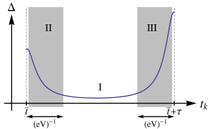
Figure 10: Sketch of the singular Fredholm determinant $\Delta[4\vartheta_{+}(\bullet;t_{k}),f_{++}]$ as function of time $t_{k}$. In region I, the asymptotic expansion (151) is valid. In regions II and III, power-law exponents are different, and $\Delta$ is given by Eqs. (156) and (158), respectively.

IV.3.1 The time integral over $t_{k}$

To perform the time integration let us consider the $t_{k}$–dependent part in Eq. (165),

$${\mathcal{J}}(t_{k})\equiv(-1)^{1+k}\Delta[4\vartheta_{+}(\bullet;t_{k}),f_{++}](f_{+}(t_{k})-f_{-}(t_{k})).$$ (166)

According to the asymptotic analysis of the previous Sec. IV.2, this integrand has the power-law singularities which give the dominant contribution to the integral (165) around $t_{k}\sim 0$ and $t_{k}\sim\tau$, provided the real part of the corresponding power-law exponents is negative. In general, for any time $t_{k}\in(0,\tau)$ the integrand is a superposition of powers-law terms,

$${\mathcal{J}}(t_{k})\sim\sum_{\{n\}}\,t_{k}^{\tilde{p}_{12}}(\tau-t_{k})^{\tilde{p}_{23}}\tau^{\tilde{p}_{13}}(eV)^{\tilde{q}_{12}}\Lambda^{\tilde{\gamma}+1},$$ (167)

where the exponent $\tilde{\gamma}\equiv\tilde{p}_{12}+\tilde{p}_{23}+\tilde{p}_{13}-\tilde{q}_{12}$ ensures the correct dimensionality (which is inverse time). As discussed previously, the sum here runs over integers $n_{1}$, $n_{2}$ or both depending on whether the time $t_{k}$ lies in the region II, III or I, respectively (see Fig. 10). For instance, in the region I the function ${\cal J}$, in accordance with Eq. (151), has the above scaling behavior with $\tilde{p}_{12}=p_{12}-1$, $\tilde{p}_{23}=p_{23}$, $\tilde{p}_{13}=p_{13}$ and $\tilde{q}_{12}=q_{12}$. Equation (150) shows that by choosing $\lvert n_{1}\rvert$ and $\lvert n_{2}\rvert$ sufficiently large, $\mathrm{Re}\,p_{12}$ and $\mathrm{Re}\,p_{23}$, respectively, can be easily made negative. Therefore the integral over $t_{k}$ will be determined by a vicinity of the end points of the time interval $(0,\tau)$.

First, let us examine the limit of short times $t_{k}\ll\tau$. One has to consider two asymptotic regions. For $\Lambda^{-1}\lesssim t_{k}\lesssim(eV)^{-1}$ (region II) we can use the short time expansion

$$f_{+}(t_{k})-f_{-}(t_{k})=\frac{i}{2\pi}\frac{e^{-ieVt_{k}}-1}{t_{k}}\simeq\frac{eV}{2\pi},$$ (168)

which gives the powers $\tilde{p}_{12}=p^{\prime}_{12}$, $\tilde{p}_{23}=0$, $\tilde{p}_{13}=p^{\prime}_{13}$, and $\tilde{q}_{12}=q^{\prime}_{12}+1$. Evaluating the $t_{k}$–integral over the region II for some given integer $n_{2}$, we find

$$\int^{1/eV}_{1/\Lambda}\!\!\!dt_{k}\,{\mathcal{J}}(t_{k}) \sim (eV\tau)^{p^{\prime}_{13}}(eV/\Lambda)^{q^{\prime}_{12}+1-p^{\prime}_{13}}$$ (169)

$$\times (\Lambda t_{k})^{p^{\prime}_{12}+1}\Biggl{\rvert}_{1/eV}^{1/\Lambda}$$

$$\sim (eV\tau)^{p^{\prime}_{13}}(eV/\Lambda)^{1+\alpha_{1}^{2}+\alpha_{1}},$$

where we kept only the dominant contribution. Here $\alpha_{1}=-2/\nu$ and, cf. Eq. (157),

$$p^{\prime}_{13}=-2\left(n_{2}-\frac{\alpha_{1}-2\beta_{1}}{2}\right)^{2}-\frac{\alpha_{1}^{2}}{2}$$ (170)

The term which gives the leading contribution to the current from the region II is then found by maximizing ${\rm Re}\,p^{\prime}_{13}$ with respect to $n_{2}$. The fact that the exponent $\Lambda$ is independent on $n_{2}$ is not a coincidence. It encodes renormalization effects due to high-energy virtual excitations. In contrast, the arbitrary integers which encode different branches of $\ln\tilde{g}$ are relevant for intermediate energies $0<\epsilon<eV$ only, and thus do not affect the high energy scale $\Lambda$.

Let us further look onto longer times, $(eV)^{-1}\lesssim t_{k}\ll\tau$ from region I, where we can approximate $f_{+}(t_{k})-f_{-}(t_{k})\sim 1/t_{k}$. Hence the powers are $\tilde{p}_{12}=p_{12}-1$, $\tilde{p}_{23}=p_{23}$, $\tilde{p}_{13}=p_{13}$, and $\tilde{q}_{12}=q_{12}$. By choosing some intermediate time scale $(eV)^{-1}\lesssim t\ll\tau$ as the upper cut-off, the integral reads

$$\int_{1/eV}^{t}\!\!\!dt_{k}\,{\mathcal{J}}(t_{k}) \sim (eV\tau)^{p_{13}+p_{23}}$$

$$\times (eV/\Lambda)^{q_{12}-p_{13}-p_{23}}(\Lambda t_{k})^{p_{12}}\Biggl{\rvert}_{1/eV}^{t}.$$

Under the assumption $\mathrm{Re}\,p_{12}<0$, the upper boundary $t$ is irrelevant. Using relations (157) and (160), we obtain exactly the same asymptotics as in Eq. (169),

$$\int_{1/eV}^{t}\!dt_{k}\,{\mathcal{J}}(t_{k})\sim(eV\tau)^{p^{\prime}_{13}}(eV/\Lambda)^{1+\alpha_{1}^{2}+\alpha_{1}}.$$ (171)

We turn now to the analysis of the integral (165) around the second singularity $t_{k}\sim\tau$. Close to this end point one has $f_{+}(t_{k})-f_{-}(t_{k})\sim\tau^{-1}$. Following the same line of reasoning as above, we consider two asymptotic regions (I and III). The time integral over the region III for a given integer $n_{1}$ yields (we recall that we consider the case $\nu\geq 2$)

$$\int^{\tau-\Lambda^{-1}}_{\tau-(eV)^{-1}} dt_{k}\,{\mathcal{J}}(t_{k})\sim(eV\tau)^{p^{\prime\prime}_{13}-1}(eV/\Lambda)^{2+\alpha_{1}^{2}+2\alpha_{1}}$$

$$\times\Bigl{(}\Lambda(\tau-t_{k})\Bigr{)}^{1+\alpha_{1}}\Bigg{\rvert}_{\tau-(eV)^{-1}}^{\tau-\Lambda^{-1}}$$

$$\sim(eV\tau)^{p^{\prime\prime}_{13}-1}(eV/\Lambda)^{1+\alpha_{1}^{2}+\alpha_{1}},$$ (172)

The exponent $p^{\prime\prime}_{13}-1$ can be read from the definition (159). It is convenient to rewrite it in the form analogous to Eq. (170),

$$p^{\prime\prime}_{13}-1=-2\left(n_{1}-\frac{\alpha_{1}+1-2\beta_{1}}{2}\right)^{2}-\frac{(\alpha_{1}+1)^{2}}{2}-1.$$ (173)

which explicitly shows that ${\rm Re}\,p^{\prime\prime}_{13}-1$ can be maximized with respect to $n_{1}$.

It remains to estimate the time integral when $t_{k}$ lies in the region I. Introducing as above some intermediate time scale $t$ satisfying $(eV)^{-1}\ll t<\tau-(eV)^{-1}$ (which in case of $\mathrm{Re}\,p_{23}<-1$ will be irrelevant as an integral boundary) one obtains

$$\int_{t}^{\tau-(eV)^{-1}}\!dt_{k}\,{\mathcal{J}}(t_{k})\sim(eV\tau)^{p^{\prime\prime}_{13}-1}(eV/\Lambda)^{1+\alpha_{1}^{2}+\alpha_{1}}.$$ (174)

In the following we are interested in the integers $n_{2}$ and $n_{1}$ which maximize the exponents, $\mathrm{Re}\,p^{\prime}_{13}$ and $\mathrm{Re}\,p^{\prime\prime}_{13}-1$. To this end we write $\alpha_{1}=M+m$ with $M\in\mathbb{Z}$ and $\lvert m\rvert\leq 1/2$. Then for even $M$ leading contributions come from $n_{2}=M/2$ and $n_{1}=(M+1)/2\pm 1/2$, and for odd $M$ they come from $n_{2}=M/2\pm 1/2$ and $n_{1}=(M+1)/2$. Straightforward analysis shows that for integer filling fractions $\nu\geq 2$ in all optimal contributions we have $\mathrm{Re}\,p^{\prime}_{13}\geq\mathrm{Re}\,p^{\prime\prime}_{13}-1$.

These observations lead us to the conclusion that, with all oscillatory terms $e^{ieV\tau n_{2}}e^{i\alpha_{1}\Lambda\tau}$ and $t_{k}$-independent contributions,

$$\Delta[4\bar{\vartheta}_{+},f_{+}]^{-1} \propto e^{-i\alpha_{1}(\Lambda+eV)\tau}\left(\frac{\Lambda\tau}{\pi}\right)^{\alpha_{1}^{2}},$$ (175)

taken into account, the leading terms of the $t_{k}$-integral for $\nu\geq 2$ are

$$\int_{1/\Lambda}^{\tau-1/\Lambda}dt_{k}\,{\cal J}(t_{k})/\Delta[4\bar{\vartheta}_{+},f_{+}] =\frac{\Lambda}{\pi}\ e^{-i\alpha_{1}eV\tau+i\beta_{1}eV\tau}(eV/\Lambda)^{1+\alpha_{1}}$$ (176)

$$\times\left(\sum_{n_{2}}\Gamma^{\prime}_{n_{2}}e^{ieV\tau n_{2}}(eV\tau)^{p^{\prime}_{13}+\alpha_{1}^{2}}+\sum_{n_{1}}\Gamma^{\prime\prime}_{n_{1}}\left(e^{-ieV\tau}-1\right)e^{ieV\tau n_{1}}(eV\tau)^{p^{\prime\prime}_{13}-1+\alpha_{1}^{2}}\right)$$

where $\Gamma^{\prime}_{n_{2}}$ and $\Gamma^{\prime\prime}_{n_{1}}$ are some unknown dimensionless constants. This expansion contains all terms in leading order of $(eV/\Lambda)$ (also those subleading in $(eV\tau)$).

IV.3.2 Action ${\cal A}^{(0)}$ in the absence of tunneling

Let us now evaluate the action of the system when inter-edge tunneling is absent,

$$i{\cal A}^{(0)}={\rm Tr}{\rm Ln}\,\left[\mathds{1}-\hat{f}+e^{2i\hat{\vartheta}^{q}}\hat{f}\right]-2i{\rm Tr}\hat{\vartheta}^{q}f_{0}.$$ (177)

In this subsection the traces extend over all $\nu$ upper and $\nu$ lower inner channels. We combined all $2\nu$ distribution functions $f_{\lambda}$ and phases $\vartheta^{q}_{\lambda}$ into $2\nu\times 2\nu$-matrices $\hat{f}$ and $\hat{\vartheta}^{q}$. Due to the Dzyaloshinskii-Larkin theorem we anticipate that only first-and-second-order-in-$\vartheta$ terms are non-vanishing for the action above (it is worth reminding here that throughout this section the distribution functions were assumed to be the Fermi-like). Hence we expand,

$$i{\cal A}^{(0)} ={\rm Tr}\left[{\rm Ln}\,\left[\mathds{1}+\left(2i\hat{\vartheta}^{q}-2\hat{\vartheta}^{q2}\right)\hat{f}\right]-2i\hat{\vartheta}^{q}f_{0}\right]$$

$$=2i{\rm Tr}\,\hat{\vartheta}^{q}\left(\hat{f}-f_{0}\right)-2{\rm Tr}\,\,\hat{\vartheta}^{q}(\mathds{1}-\hat{f})\hat{\vartheta}^{q}\hat{f}.$$ (178)

Consider now three local operators $A$, $B$, $C$, where by definition $A(t_{1},t_{2})=A(t_{1})\delta(t_{1}-t_{2})$ etc. Evaluating the following trace (one should carefully take into account here the non-local in time structure of the Fermi-distribution function), one obtains

$${\rm Tr}\,_{t}A[B,f_{0}]C =\int\!\!dt_{2}\,\lim_{t_{1}\to t_{2}}A(t_{1})\frac{i}{2\pi}\frac{B(t_{1})-B(t_{2})}{t_{1}-t_{2}+i0}C(t_{2})$$

$$=\frac{i}{2\pi}\int\!\!dt\,A(t)\dot{B}(t)C(t).$$ (179)

For Fermi-like non-equilibrium distribution functions, $f_{1}(t)=e^{-ieV_{1}t}f_{0}(t)$, the above relation implies

$${\rm Tr}_{t}A(f_{1}-f_{0})C=\frac{eV_{1}}{2\pi}\int\!\!dt\,A(t)C(t).$$ (180)

Let us assume that among the channels belonging to the upper edge of the MZI, the outer channel is biased by $V$ and all the rest ones by $V_{0}$. At the same time, all channels on the lower edge are grounded. This gives the first, “zero mode” contribution to the action,

$$2i{\rm Tr}\hat{\vartheta}^{q}\left(\hat{f}-f_{0}\right)=i\frac{e\left[V+(\nu-1)V_{0}\right]\tau}{2\pi}\ 2\bar{\vartheta}_{+}.$$ (181)

The quadratic contribution to the action $i{\cal A}^{(0)}$ is UV divergent and needs to be cutoff by at the scale $\Lambda\sim\omega_{c}$, yielding

$$-2{\rm Tr}\vartheta^{q}\left(\mathds{1}-\hat{f}\right)\vartheta^{q}\hat{f}=-\frac{2\nu\bar{\vartheta}^{2}_{+}}{\pi^{2}}\ln\omega_{c}\tau=-\frac{2}{\nu}\ln\omega_{c}\tau.$$ (182)

In passing we note, that since ${\cal A}^{(0)}$ is a purely Gaussian contribution, it can be equivalently evaluated by averaging the phase $e^{i{\cal A}^{(0)}}=\left\langle e^{i\vartheta^{f}_{+}(0)-i\vartheta^{b}_{-}(0)}\right\rangle_{0}$ over the Gaussian action of the MZI in the limit $T_{1}\to 0$.

IV.3.3 Current, Conductivity and Visibility

The results of previous subsections enable us to evaluate the Aharonov-Bohm current in the MZI. Setting the voltage of all outer channels to zero, $V=0$, and defining the exponents

$$p^{\prime}(n_{2}) \equiv-2\left(n_{2}-\frac{\alpha_{1}-2\beta_{1}}{2}\right)^{2}+1+\frac{\alpha_{1}^{2}}{2}+\alpha_{1},$$ (183)

$$p^{\prime\prime}(n_{1}) \equiv-2\left(n_{1}-\frac{\alpha_{1}+1-2\beta_{1}}{2}\right)^{2}-\frac{1}{2}+\frac{\alpha_{1}^{2}}{2},$$ (184)

one can represent the coherent current contribution in the form

$$I_{\rm coh}=2\mathrm{Re}\,I_{+-}=\frac{e}{2\pi\tau}(R_{1}T_{1}R_{2}T_{2})^{1/2}2\,\mathrm{Re}\,e^{i\Phi}\ {\mathcal{I}}_{0},$$ (185)

where ${\mathcal{I}}_{0}$ is the normalized amplitude of the Aharonov-Bohm current. Collecting Eqs. (163), (176), (181) and (182) together, we finally arrive at

$${\mathcal{I}}_{0}=2e^{-2\pi i/\nu}e^{i(\beta_{1}+1/\nu)eV\tau}\times\left(\sum_{n_{2}}\Gamma^{\prime}_{n_{2}}e^{in_{2}eV\tau}\left(eV\tau\right)^{p^{\prime}(n_{2})}+\sum_{n_{1}}\Gamma^{\prime\prime}_{n_{1}}e^{in_{1}eV\tau}\left(e^{-ieV\tau}-1\right)\left(eV\tau\right)^{p^{\prime\prime}(n_{1})}\right).$$ (186)

The following table shows the power-law exponents corresponding to the terms which give the dominant contribution to the series (186) at each filling factor $\nu$:

$\nu$	leading powers
2	$p^{\prime}(0)=p^{\prime}(-1)=0=p^{\prime\prime}(0)$
3	$p^{\prime}(-1$) and $p^{\prime}(0)$
$\geq 4$	$p^{\prime}(0)$ and $p^{\prime\prime}(0)$ if $T_{1}<1/2$ or $p^{\prime\prime}(1)$ if $T_{1}>1/2$

Taking these leading terms into account we obtain the results presented in Sect. II.2, namely Eq. (9) with the exponents (II.2) and (15). We have also checked the validity of analytical asymptotics (186) by straightforward numerical evaluation of Eq. (165) for the AB current. The perfect agreement between the analytical and numerical approaches, demonstrated in Fig. 4, provides additional support towards the conjecture of Ref. Protopopov et al., 2012.

We close this section by providing the reader with a qualitative physical picture, underlying the result (186). We begin with inspection of the phase pulse $\delta(t)=4\vartheta_{+}(t;t_{k})$ which according to our discussion in Sec. IV.2 determines the resolvent (${\cal D}^{-1}$) of the counting operator (see Fig. 9). First, we note that in our model of the maximally long-ranged Coulomb interaction the counting phase $4\vartheta_{+}(t)=(4\pi/\nu)q(t)$, with $q(t)$ being the “background” charge on the upper arm of the MZI. The phase $\delta(t)$ is different from $4\vartheta_{+}(t)$ by the $2\pi$-pulse of the duration $t_{k}$, which describes injection of the interfering “transport” electron at time $\bar{t}=0$ into the interferometer via the QPC1 and its annihilation at time $t_{k}$ (the electrons leaves the MZI through the QPC2). As we see it from the calculations of the Sec. IV.3.1, in the high-voltage limit $eV\tau\gg 1$, the critical exponents $p^{\prime}$ are associated with many-particle scattering processes with short $t_{k}$, $t_{k}\simeq\hbar/eV$. We can interpret it as the event when one electron enters the MZI through the QPC1 and another electron leaves the MZI shortly afterward on a time scale $\sim\hbar/eV$ via the QPC2. The possibility for an electron to propagate through the system in a time $t_{k}\ll\tau$ is due to the long-range nature of Coulomb interaction in our model (a similar situation will occur in a model with a strong short-ranged interaction, where such a process can be mediated by the exchange of plasmons, which have a velocity exceeding by far the bare velocity of electrons). On the contrary, the second critical exponent $p^{\prime\prime}$ is due to many-body scattering events with time $t_{k}\simeq\tau$. In this case the MZI is excited into a state with an extra electron for a long time $\tau\gg\hbar/eV$ (it will be, e.g., the only possibility in the limit of weak short-ranged interaction when the behavior of the MZI is very close to the one with non-interacting electrons).

Next, we associate the integers $n_{1}$ and $n_{2}$ with the number of inelastically excited electron-hole pairs on the MZI in the corresponding time intervals (at $0<t<t_{k}$ and $t_{k}<t<\tau$, respectively). More precisely, one can interpret each term in the asymptotic expansion for the current ${\cal J}(t_{k})$ as the product of forward (electron-like) and backward (hole-like) many-particle scattering amplitudes, $A^{b}(\{n^{-}\};t_{k})\times A^{f}(\{n^{+}\};t_{k})$. An electron, propagating through the upper arm of the MZI leaves a trace in the bath of particle-hole excitations, which is encoded in the numbers $n^{+}_{1}$ and $n^{+}_{2}$ of the excited electron-hole pairs after the electron’s injection and annihilation. The dominant e-h pairs correspond to excitations from one Fermi edge to the other, so that the typical energy of an electron-hole pair is $\hbar\omega\simeq eV$. The corresponding many-particle amplitude should behave as

$$A^{f}(\{n^{+}\};t_{k})\sim e^{-in^{+}_{1}eVt_{k}-in_{2}^{+}eV(\tau-t_{k})}.$$

Similarly, the backward amplitude is characterized by numbers $n_{1}^{-}$ and $n^{-}_{2}$. In the case when the relative numbers $n_{1}=n^{+}_{1}-n^{-}_{1}$ and $n_{2}=n^{+}_{2}-n^{-}_{2}$ between the forward and backward scattering amplitudes are non-zero one obtains an interference term in the current with a phase which is linear in voltage. The two dominant terms with inequivalent phases in the series for the current $I_{+-}$ produce the lobe pattern in the visibility of the Aharonov-Bohm oscillations. For example, at $\nu=3$ such two terms are those corresponding to scattering processes characterized by the short time $t_{k}\sim\hbar/eV$ but having different numbers $n_{2}=-1$ and $n_{2}=0$, resp.

V Numerical approach

In this section we present a numerical evaluation scheme for the interference current. Results, obtained within this scheme, corroborate and complement the analytical study of Sec. IV based on the particular form of the Fredholm counting operator ${\cal D}$. After making a few introductory remarks regarding the numerical formula for the Aharonov-Bohm current, which is suitable for a practical implementation, we consider two cases when we did not succeed to obtain the analytical asymptotics and had to evaluate the Fredholm determinants numerically. This is, first, the case of non-equilibrium incoming distribution (Sec. V.1) and, second, the regime of intermediate interaction strength $E_{c}\tau\sim 1$ (Sec. V.2).

As argued in Sec. IV.3, the interference current is obtained from Eq. (46) by dropping the divergent $\bar{t}$-integral and putting $\bar{t}=0$. For the purpose of the present section we rewrite this formula in the equivalent form

$$I_{+-}=I_{+-}^{({\rm eq})}\left[{\rm Det}\,\tilde{\cal D}\right]_{\rm norm}\left[\left\langle+\right\rvert\tilde{f}\tilde{\cal D}^{-1}(0,0)\left\lvert-\right\rangle\right]_{\rm norm}.$$ (187)

Here,

$$I_{+-}^{({\rm eq})}=-i\left(R_{2}T_{2}\right)^{1/2}e^{i\Phi}e^{i{\cal A}_{{\rm ferm}}+i\delta{\cal A}}\left\langle+\right\rvert\tilde{f}\tilde{\cal D}^{-1}(0,0)\left\lvert-\right\rangle\Big{\rvert}_{eV=\epsilon_{0}}$$

denotes the near-to-equilibrium current, evaluated at very small voltages $\epsilon_{0}\tau\ll 1$, while the label “norm” refers to quantities which are normalized with respect to near-to-equilibrium values, i.e.

$$\left[{\rm Det}\,\tilde{\cal D}\right]_{\rm norm}={{\rm Det}\,\tilde{\cal D}}/{{\rm Det}\,\tilde{\cal D}\Big{\rvert}_{eV=\epsilon_{0}}}.$$

The density matrix $\tilde{f}$ can be removed from the matrix element appearing in Eq. (187) by using a relation

$${\mathds{1}}-\tilde{\cal D}^{-1}=\left(e^{2i\hat{\vartheta}^{q}}-{\mathds{1}}\right)\tilde{f}\tilde{\cal D}^{-1},$$

which leads to

$$\left[\left\langle+\right\rvert\tilde{f}\tilde{\cal D}^{-1}(0,0)\left\lvert-\right\rangle\right]_{\rm norm}=\frac{\left\langle+\right\rvert\tilde{\cal D}^{-1}(0,0)\left\lvert-\right\rangle}{\left\langle+\right\rvert\tilde{\cal D}^{-1}(0,0)\left\lvert-\right\rangle\Big{\rvert}_{eV=\epsilon_{0}}}.$$

By solving an appropriate Riemann-Hilbert problem we were able to show that close to equilibrium all effects of non-equilibrium and interaction, like dephasing and renormalization, are absent for the Aharonov-Bohm current. In agreement with the Landauer-Büttiker result it depends linearly on voltage, thus

$$I^{({\rm eq})}_{+-}=\left(R_{1}T_{1}R_{2}T_{2}\right)^{1/2}e^{i\Phi}\ \frac{e\epsilon_{0}}{2\pi}.$$

Corrections to this equilibrium expression are encoded in the normalized terms in Eq. (187). By discretizing the integral operator ${\cal D}$ the latter become amenable to numerical evaluation. Below we discuss two different discretization schemes. In practice, the choice between two depends mainly on the strength of Coulomb interaction.

V.1 Non-equilibrium incoming distribution

We consider the situation when the incoming electron beam is diluted and is driven out of equilibrium even before scattering at the first QPC. More specifically, we focus on the setup (that has been realized experimentally) with an additional QPCO with a transparency $0<R<1$ placed outside of the interferometer and diluting the incoming beam. The incoming then distribution function acquires the double-step form, $f_{+}(\epsilon)=T_{0}\theta(-\epsilon)+R_{0}\theta(eV-\epsilon)$.

As in Sec. IV, we focus here on the limit of strong interaction $E_{c}\tau\gg 1$, where the counting phase (58) is a window function and the counting operator $\cal D$ is of block Toeplitz form with a two-channel structure. Note that its decomposition into single-channel operators that was performed in Sec. IV.1 requires trivial incoming distribution functions $f_{+}$, $f_{-}$, i.e. zero-temperature Fermi distributions, possibly with different chemical potentials. Thus the non-equilibrium form of $f_{+}$ constitutes an obstacle for a further analytical evaluation. At this stage, we do not know whether there is an analytical way to overcome this problem. We thus resort to a numerical evaluation of the determinants.

To proceed numerically we use the same discretization procedure as in Sec. IV.2, where the energy cutoff $\Lambda$ is introduced and the symbol $\hat{g}(\epsilon)$ of $\tilde{\cal D}$ is required to satisfy periodic boundary conditions in energy domain,

$$\hat{g}(\epsilon)=e^{i\hat{\bar{\vartheta}}\epsilon/\Lambda}\left[{\mathds{1}}+(e^{2i\hat{\bar{\vartheta}}}-{\mathds{1}})\tilde{f}(\epsilon)\right].$$

Now the symbol $\hat{g}(\epsilon)\in{\mathbb{C}}^{2\times 2}$ has an additional $2\times 2$-channel structure, the same holds for the diagonal matrix $\hat{\bar{\vartheta}}$ with diagonal entries $\bar{\vartheta}_{+}$, $\bar{\vartheta}_{-}$. In the discretized representation the counting operator $\tilde{\cal D}$ then reads

$$\tilde{\mathcal{D}}_{j-k} =\int_{-\Lambda}^{\Lambda}\!\frac{{\rm d}\epsilon}{2\Lambda}\,e^{-i\epsilon\frac{\pi}{\Lambda}[j-k]}\ \hat{g}(\epsilon)$$

$$=\frac{i}{2\pi}\frac{e^{2i\hat{\bar{\vartheta}}}-{\mathds{1}}}{j-k-\hat{\bar{\vartheta}}/\pi}\begin{pmatrix}R_{1}R_{0}e^{-i\pi\frac{eV}{\Lambda}\left[j-k-\bar{\vartheta}_{+}/\pi\right]}+T_{0}+T_{1}R_{0}&i\left(R_{1}T_{1}\right)^{1/2}R_{0}\left(e^{-i\pi\frac{eV}{\Lambda}\left[j-k-\bar{\vartheta}_{+}/\pi\right]}-1\right)\\ -i\left(R_{1}T_{1}\right)^{1/2}R_{0}\left(e^{-i\pi\frac{eV}{\Lambda}\left[j-k+\bar{\vartheta}_{+}/\pi\right]}-1\right)&T_{1}R_{0}e^{-i\pi\frac{eV}{\Lambda}\left[j-k+\bar{\vartheta}_{+}/\pi\right]}+R_{1}+T_{1}T_{0}\end{pmatrix}.$$ (188)

The resulting visibility which follows from the above approach is shown and discussed in Sec. II.2, see Fig. 5. A good convergence was already achieved for moderate matrix sizes with $N=\Lambda\tau/\pi\sim 100$. While we do not have a complete analytical form of the Aharonov-Bohm current in this case, the dephasing rate can be deduced from the leading large-$\tau$ asymptotic behavior of ${\rm Det}\,\tilde{\cal D}\sim e^{-\tau/\tau_{\phi}}$. Making use of the results for the block Toeplitz determinants Widom (1974), we arrive at

$$\tau_{\phi}^{-1} =-\int\!\frac{{\rm d}\epsilon}{2\pi}\,\mathrm{Re}\,\ln\det\left[{\mathds{1}}-\hat{f}+s_{1}^{\dagger}e^{2i\hat{\bar{\vartheta}}}s_{1}\hat{f}\right]$$ (189)

$$=-\frac{eV}{2\pi}\mathrm{Re}\,\ln\left[T_{0}+R_{0}\left(R_{1}e^{-i2\pi/\nu}+T_{1}e^{i2\pi/\nu}\right)\right]$$

In the case $\nu=2$ the dephasing rate is simplified to $\tau_{\phi}^{-1}=-({eV}/{2\pi})\ln|2R_{0}-1|$, as has been already mentioned in Sec. II.2.

V.2 Intermediate interaction strength

We now consider the discretization scheme applicable in the case of a moderate charging energy, $E_{c}\tau\sim 1$. In this general case the correlation function (55) has to be evaluated numerically (see, e.g., Fig. 8 in Sec. III.2 which shows the result for $\omega_{c}\tau=25$). Owing to finite $E_{c}$, the counting phase $\vartheta_{+}(t)$ is not a piecewise constant function of time anymore, but rather acquires oscillations in time. As an illustration, the phase $\theta_{+}(t)$ is plotted in Fig. 7 for two different charging energies. Thus, the situation is different from the previous subsection, since the counting operator is no longer of Toeplitz form. Despite this complication, a numerical treatment based on Eq. (187) is nevertheless possible, but a time discretization of the kernel ${\cal D}(t,t^{\prime})$ has to be performed directly in the time domain without any reference to the conjugate energy representation. To this end, we rely on the approach similar to the one used in Ref. Snyman and Nazarov, 2007 (see Supplemental Material of that work) and interpret the zero-temperature Fermi distribution function $f_{0}$ in terms of the Cauchy principal value and the Dirac delta distribution,

$$f_{0}(t)=\frac{i}{2\pi}\frac{1}{t+i0}=\frac{i}{2\pi}\mathcal{P}\frac{1}{t}+\frac{1}{2}\delta(t).$$

Consequently, the discretization of the non-equilibrium single-particle density matrix, $\tilde{f}_{jk}=\hat{s}_{1}\hat{f}^{1}(t_{i},t_{j})\hat{s}_{1}^{\dagger}\Delta t$, with $t_{j}=(j-1)\Delta t$ and $\Delta t=\pi/\Lambda$ yields

$$\tilde{f}_{jk} =\left(1-\delta_{jk}\right)\frac{i}{2\pi}\frac{1}{j-k}+\frac{1}{2}\delta_{jk}+\begin{pmatrix}R_{1}&\left(R_{1}T_{1}\right)^{1/2}\\ -i\left(R_{1}T_{1}\right)^{1/2}&T_{1}\end{pmatrix}\left[\left(1-\delta_{jk}\right)\frac{i}{2\pi}\frac{e^{-i\pi\frac{eV}{\Lambda}(j-k)}-1}{j-k}+\delta_{jk}\frac{eV}{2\Lambda}\right],$$

with $\Lambda\gg E_{c}$ being a high-energy cut-off. Making use of above expression one can further construct the discretized matrix of the counting operator

$$\tilde{\cal D}_{jk}=\delta_{jk}{\mathds{1}}_{2}-\left(e^{2i\hat{\vartheta}^{q}(t_{j})}-{\mathds{1}}_{2}\right)\circ\tilde{f}_{jk}$$ (190)

where “$\circ$” denotes matrix multiplication with respect to channel indices.

The discretized form outlined above is very general, since it allows for arbitrary time-dependent phases. Note, however, that for the case of window-function time dependence of the “counting” phase (i.e., Toeplitz case) this regularization yields a result which is manifestly $2\pi$ periodic in $2\vartheta^{q}$, with nonanalyticity at points $(2n+1)\pi$. This should be contrasted to the analytic and non-periodic behavior of the Toeplitz determinant within the proper regularization discussed above. The corresponding difference between the present problem and that of FCS has already been mentioned in the end of Sec. IV.1.1. We have checked that for $|2\vartheta^{q}|<\pi$ both regularization schemes, Eqs. (V.1) and (190) produce identical results, although the convergence of the second scheme is generally worse.

In the case of a finite charging energy the phase changes continuously with time, and there is no more problem with the regularization (190), independently of how large the values acquired by the phase are. We used the matrix size $N=\Lambda\tau/\pi\sim 500$, which was sufficient to obtain numerical results for the visibility at $E_{c}\sim 1/\tau$ with good precision. The results were presented and discussed in Sec. II.3.

Finally, we have calculated analytically the long-$\tau$ asymptotics of the action ${\cal A}_{\rm ferm}=-i\ln{\rm Det}{\cal D}$, which gives the out-of-equilibrium dephasing rate (19) of the Aharonov-Bohm oscillations.

VI Summary

In this paper, we have discussed an exactly solvable model of a quantum Hall electronic Mach-Zehnder interferometer for arbitrary integer filling factor $\nu$. The model is specified by a form of e-e interaction restricted to the inner part of the interferometer and two single-particle scattering matrices of quantum point contacts (QPCs). Our main results can be summarized as follows:

1. Making use of the non-equilibrium functional bosonization approach, we have established the exact solution of the above model in terms of the resolvent of the Fredholm integral operator — single-particle “counting operator” ${\cal D}$, which is related to the problem of electron full counting statistics (FCS). The time-dependent scattering phase $\vartheta_{+}(t)$ of the operator ${\cal D}$ encodes all information about the interaction in the system. The link between the initial many-body problem with Coulomb interaction and single-particle quantities is established by virtue of the real-time instanton technique which becomes exact for the specific type of the Keldysh action describing the MZI.

2. The focus of our study was on the model with “maximally long-range” Coulomb interaction characterized by the electrostatic charging energy $E_{c}$. In the limit of strong interaction $E_{c}\gg 1/\tau$ (here $\tau$ is the electron flight time through the MZI) the scattering phase $\vartheta_{+}(t)$ becomes a piecewise constant “window” function and the operator $\cal D$ simplifies to the block Toeplitz form. In the absence of external dephasing, we were able to get rid of the matrix structure of $\cal D$ and have expressed the result in terms of singular Fredholm determinants that may be viewed as a generalization of Toeplitz determinants with Fisher-Hartwig singularities. This has allowed us to evaluate the Aharonov-Bohm (AB) conductance in a closed analytical form. At a moderate charging energy $E_{c}\sim 1/\tau$ and/or in the situation when the incoming distribution is made non-equilibrium by an additional QPC placed outside of MZI, we have obtained the results for the visibility by evaluating the determinants numerically.

3. Results of our theory at $E_{c}\sim 1/\tau$ match in all principal aspects the experimental observation in many designs of Mach-Zehnder interferometers at filling factor $\nu$=2. If the transmission coefficient $T_{1}$ of the QPC1 is close to $1/2$ the visibility dependence on external bias shows a number of “lobes”, their amplitude is being suppressed with the increase of voltage. The AB-phase dependence is close to a piecewise constant function with jumps equal to $\pi$ at minima of the visibility. The visibility is further suppressed when the MZI is subjected to an out-of-equilibrium shot noise, generated by the QPC0 placed outside the interferometer. We have quantified the dephasing rate $1/\tau_{\phi}$ which governs the decay of AB oscillations with bias in terms the transmission of QPCs, filling factor $\nu$ and the strength of e-e interaction $E_{c}\tau$.

4. Our analytical results in the limit of strong interaction $E_{c}\tau\gg 1$ show an intimate connection between the observed “lobe” structure in the visibility, on one hand, and multiple branches in the asymptotics of singular integral determinants, on the other hand. In more physical terms, this is the many-body interference effect resulting from the quantum superposition of many-particle scattering amplitudes with the mutual phase differences which are linear in external bias. We derived the non-equilibrium quantum critical exponents, which depend both on the transmission $T_{1}$ and the filling factor $\nu$. They are attributed to the Anderson orthogonality catastrophe under out-of-equilibrium conditions and describe the power-law dependence of the above many-particle amplitudes on voltage.

Before closing, we mention some future research directions. An extension of the presented approach to the fractional quantum Hall edge states devices, comprising two (or more) QPCs which couple the co-propagating edge modes, would be of great interest. Another important research direction is the analysis of the asymptotic behavior of block Toeplitz determinants with Fisher-Hartwig singularities (and, more generally, block determinants, with symbols that have multiple energy and time singularities). This would not only permit to obtain closed analytical results in the model with moderate interaction strength but would likely have multiple further applications.

VII Acknowledgments

This work was supported by the collaborative research grant SFB/TR12 of the Deutsche Forschungsgemeinschaft and by German-Israeli Foundation. D.B. is grateful to the TKM Institute at KIT for the hospitality.

References

- Ji et al. (2003) Y. Ji, Y. C. Chung, D. Sprinzak, M. Heiblum, D. Mahalu, and H. Shtrikman, Nature (London) 422, 415 (2003).
- Neder et al. (2006) I. Neder, M. Heiblum, Y. Levinson, D. Mahalu, and V. Umansky, Phys. Rev. Lett. 96, 016804 (2006).
- Neder et al. (2007a) I. Neder, M. Heiblum, D. Mahalu, and V. Umansky, Phys. Rev. Lett. 98, 036803 (2007a).
- Neder et al. (2007b) I. Neder, F. Marquardt, M. Heiblum, D. Mahalu, and V. Umansky, Nat. Phys. 3, 534 (2007b).
- Roulleau et al. (2007) P. Roulleau, F. Portier, D. C. Glattli, P. Roche, A. Cavanna, G. Faini, U. Gennser, and D. Mailly, Phys. Rev. B 76, 161309 (2007).
- Roulleau et al. (2008a) P. Roulleau, F. Portier, P. Roche, A. Cavanna, G. Faini, U. Gennser, and D. Mailly, Phys. Rev. Lett. 100, 126802 (2008a).
- Roulleau et al. (2008b) P. Roulleau, F. Portier, P. Roche, A. Cavanna, G. Faini, U. Gennser, and D. Mailly, Phys. Rev. Lett. 101, 186803 (2008b).
- Roulleau et al. (2009) P. Roulleau, F. Portier, P. Roche, A. Cavanna, G. Faini, U. Gennser, and D. Mailly, Phys. Rev. Lett. 102, 236802 (2009).
- Litvin et al. (2007) L. V. Litvin, H.-P. Tranitz, W. Wegscheider, and C. Strunk, Phys. Rev. B 75, 033315 (2007).
- Litvin et al. (2008) L. V. Litvin, A. Helzel, H.-P. Tranitz, W. Wegscheider, and C. Strunk, Phys. Rev. B 78, 075303 (2008).
- Litvin et al. (2010) L. V. Litvin, A. Helzel, H.-P. Tranitz, W. Wegscheider, and C. Strunk, Phys. Rev. B 81, 205425 (2010).
- Bieri et al. (2009) E. Bieri, M. Weiss, O. Göktas, M. Hauser, C. Schönenberger, and S. Oberholzer, Phys. Rev. B 79, 245324 (2009).
- Huynh et al. (2012) P.-A. Huynh, F. Portier, H. le Sueur, G. Faini, U. Gennser, D. Mailly, F. Pierre, W. Wegscheider, and P. Roche, Phys. Rev. Lett. 108, 256802 (2012).
- Helzel et al. (2012) A. Helzel, L. V. Litvin, I. P. Levkivskyi, E. V. Sukhorukov, W. Wegscheider, and C. Strunk, arXiv:1211.5951 (2012).
- Aronov and Sharvin (1987) A. G. Aronov and Y. V. Sharvin, Rev. Mod. Phys. 59, 755 (1987).
- Seelig and Büttiker (2001) G. Seelig and M. Büttiker, Phys. Rev. B 64, 245313 (2001).
- Seelig et al. (2003) G. Seelig, S. Pilgram, A. N. Jordan, and M. Büttiker, Phys. Rev. B 68, 161310 (2003).
- Marquardt and Bruder (2004a) F. Marquardt and C. Bruder, Phys. Rev. Lett. 92, 056805 (2004a).
- Marquardt and Bruder (2004b) F. Marquardt and C. Bruder, Phys. Rev. B 70, 125305 (2004b).
- Förster et al. (2005) H. Förster, S. Pilgram, and M. Büttiker, Phys. Rev. B 72, 075301 (2005).
- Neder and Marquardt (2007) I. Neder and F. Marquardt, New J. Phys. 9, 112 (2007).
- Ludwig and Mirlin (2004) T. Ludwig and A. D. Mirlin, Phys. Rev. B 69, 193306 (2004).
- Le Hur (2005) K. Le Hur, Phys. Rev. Lett. 95, 076801 (2005).
- Le Hur (2006) K. Le Hur, Phys. Rev. B 74, 165104 (2006).
- Texier and Montambaux (2005) C. Texier and G. Montambaux, Phys. Rev. B 72, 115327 (2005).
- Dmitriev et al. (2010) A. P. Dmitriev, I. V. Gornyi, V. Y. Kachorovskii, and D. G. Polyakov, Phys. Rev. Lett. 105, 036402 (2010).
- Chalker et al. (2007) J. T. Chalker, Y. Gefen, and M. Y. Veillette, Phys. Rev. B 76, 085320 (2007).
- Sukhorukov and Cheianov (2007) E. V. Sukhorukov and V. V. Cheianov, Phys. Rev. Lett. 99, 156801 (2007).
- Neder and Ginossar (2008) I. Neder and E. Ginossar, Phys. Rev. Lett. 100, 196806 (2008).
- Youn et al. (2008) S.-C. Youn, H.-W. Lee, and H.-S. Sim, Phys. Rev. Lett. 100, 196807 (2008).
- Levkivskyi and Sukhorukov (2008) I. P. Levkivskyi and E. V. Sukhorukov, Phys. Rev. B 78, 045322 (2008).
- Levkivskyi and Sukhorukov (2009) I. P. Levkivskyi and E. V. Sukhorukov, Phys. Rev. Lett. 103, 036801 (2009).
- Kovrizhin and Chalker (2009) D. L. Kovrizhin and J. T. Chalker, Phys. Rev. B 80, 161306 (2009).
- Kovrizhin and Chalker (2010) D. L. Kovrizhin and J. T. Chalker, Phys. Rev. B 81, 155318 (2010).
- Schneider et al. (2011) M. Schneider, D. A. Bagrets, and A. D. Mirlin, Phys. Rev. B 84, 075401 (2011).
- Rufino et al. (2012) M. J. Rufino, D. L. Kovrizhin, and J. T. Chalker, arXiv:1209.1127 (2012).
- Altimiras et al. (2010a) C. Altimiras, H. le Sueur, U. Gennser, A. Cavanna, D. Mailly, and F. Pierre, Nat. Phys. 6, 34 (2010a).
- Altimiras et al. (2010b) C. Altimiras, H. le Sueur, U. Gennser, A. Cavanna, D. Mailly, and F. Pierre, Phys. Rev. Lett. 105, 226804 (2010b).
- le Sueur et al. (2010) H. le Sueur, C. Altimiras, U. Gennser, A. Cavanna, D. Mailly, and F. Pierre, Phys. Rev. Lett. 105, 056803 (2010).
- Kovrizhin and Chalker (2012) D. L. Kovrizhin and J. T. Chalker, Phys. Rev. Lett. 109, 106403 (2012).
- Levkivskyi and Sukhorukov (2012) I. P. Levkivskyi and E. V. Sukhorukov, Phys. Rev. B 85, 075309 (2012).
- Wen (2004) X.-G. Wen, Quantum Field Theory of Many-body Systems (Oxford University Press, Oxford, 2004).
- Gutman et al. (2008) D. B. Gutman, Y. Gefen, and A. D. Mirlin, Phys. Rev. Lett. 101, 126802 (2008).
- Gutman et al. (2010a) D. B. Gutman, Y. Gefen, and A. D. Mirlin, Europhys. Lett. 90, 37003 (2010a).
- Gutman et al. (2010b) D. B. Gutman, Y. Gefen, and A. D. Mirlin, Phys. Rev. B 81, 085436 (2010b).
- D.A.Abanin and Levitov (2005) D.A.Abanin and L. Levitov, Phys.Rev. Lett. 94, 186803 (2005).
- Fendley et al. (1995) P. Fendley, A. W. W. Ludwig, and H. Saleur, Phys. Rev. B 52, 8934 (1995).
- Ponomarenko and Averin (2009) V. V. Ponomarenko and D. V. Averin, Phys. Rev. B 80, 201313 (2009).
- Ponomarenko and Averin (2010) V. V. Ponomarenko and D. V. Averin, Phys. Rev. B 82, 205411 (2010).
- Ngo Dinh et al. (2012) S. Ngo Dinh, D. A. Bagrets, and A. D. Mirlin, Annals of Physics 327, 2794 (2012).
- Levitov et al. (1996) L. S. Levitov, H. Lee, and G. B. Lesovik, Journal of Mathematical Physics 37, 4845 (1996).
- Protopopov et al. (2012) I. V. Protopopov, D. B. Gutman, and A. D. Mirlin, arXiv:1212.0708 (2012).
- Note (1) We note that in view of the specific chiral geometry of the MZI the charge from the internal interacting region of the interferometer can always freely leak into the source or drain, and thus the issue of Coulomb blockade phenomenon is not relevant here.
- Aleiner and Glazman (1994) I. L. Aleiner and L. I. Glazman, Phys. Rev. Lett. 72, 2935 (1994).
- Kamenev and Levchenko (2009) A. Kamenev and A. Levchenko, Advances in Physics 58, 197 (2009).
- Kamenev (2011) A. Kamenev, Field Theory of Non-Equilibrium Systems (Cambridge University Press, Cambridge, 2011).
- Ngo Dinh et al. (2010) S. Ngo Dinh, D. A. Bagrets, and A. D. Mirlin, Phys. Rev. B 81, 081306 (R) (2010).
- Gutman et al. (2010c) D. B. Gutman, Y. Gefen, and A. D. Mirlin, Phys. Rev. Lett. 105, 256802 (2010c).
- Fisher and Hartwig (1968) M. E. Fisher and R. E. Hartwig, Advan. Chem. Phys. 15, 333 (1968).
- Krasovsky (2011) I. Krasovsky, Progress in Probability 64, 305 (2011).
- Gutman et al. (2011) D. B. Gutman, Y. Gefen, and A. D. Mirlin, J. Phys. A: Math. Theor 44, 165003 (2011).
- Protopopov and Mirlin (2011) D. B. Protopopov, I.V. Gutman and A. D. Mirlin, J. Stat. Mech. , P11001 (2011).
- Deift et al. (2011) P. Deift, A. Its, and K. I., Ann. Math. 174-2, 1243 (2011).
- Widom (1974) H. Widom, Advances in Math. 13, 284 (1974).
- Snyman and Nazarov (2007) I. Snyman and Y. V. Nazarov, Phys. Rev. Lett. 99, 096802 (2007).