Negative Energy Seen By Accelerated Observers

Abstract

The sampled negative energy density seen by inertial observers, in arbitrary quantum states is limited by quantum inequalities, which take the form of an inverse relation between the magnitude and duration of the negative energy. The quantum inequalities severely limit the utilization of negative energy to produce gross macroscopic effects, such as violations of the second law of thermodynamics. The restrictions on the sampled energy density along the worldlines of accelerated observers are much weaker than for inertial observers. Here we will illustrate this with several explicit examples. We consider the worldline of a particle undergoing sinusoidal motion in space in the presence of a single mode squeezed vacuum state of the electromagnetic field. We show that it is possible for the integrated energy density along such a worldline to become arbitrarily negative at a constant average rate. Thus the averaged weak energy condition is violated in these examples. This can be the case even when the particle moves at non-relativistic speeds. We use the Raychaudhuri equation to show that there can be net defocussing of a congruence of these accelerated worldlines. This defocussing is an operational signature of the negative integrated energy density. These results in no way invalidate nor undermine either the validity or utility of the quantum inequalities for inertial observers. In particular, they do not change previous constraints on the production of macroscopic effects with negative energy, e.g., the maintenance of traversable wormholes.

I Introduction

It is well known that quantum field theory allows for the existence of negative energy density, which constitute local violations of the weak energy condition. For a recent review, see Ref. F10 . Negative energy density can arise either from boundaries, as in the Casimir effect, from background spacetime curvature, or from selected quantum states in Minkowski spacetime. The last possibility will be the focus of the present paper. It is possible to create states, such as a squeezed vacuum state of the quantized electromagnetic field, in which the energy density at a given spacetime point is arbitrarily negative. However, the duration of the negative energy is strongly constrained by quantum inequalities F78 ; F91 ; FR95 ; FR97 ; Flanagan97 ; FE98 ; P02 ; FH05 . These are restrictions on a time averaged energy density measured by an observer. (Time averaging is essential, as there is no analogous restriction on spatial averages FHR02 .) Let us consider the case of inertial observers in Minkowski spacetime, with four velocity $u^{\mu}$. If $\langle T_{\mu\nu}\rangle$ is the expectation value of the normal ordered stress tensor operator in an arbitrary quantum state, then quantum inequalities take the form

$$\int_{-\infty}^{\infty}f(\tau)\,\langle T_{\mu\nu}\rangle\,u^{\mu}u^{\nu}\,d\tau\geq-\frac{C_{0}}{{\tau_{0}}^{d}}\,.$$ (1)

Here $\tau$ is the observer’s proper time, $f(\tau)$ is a sampling function with characteristic width $\tau_{0}$, and $d$ is the number of spacetime dimensions. The dimensionless constant $C_{0}$ depends upon the form of the sampling function, and is typically small compared to unity. In the limit $\tau_{0}\rightarrow\infty$, Eq. (1) becomes the averaged weak energy condition

$$\int_{-\infty}^{\infty}\langle T_{\mu\nu}\rangle\,u^{\mu}u^{\nu}\,d\tau\geq 0\,,$$ (2)

which states that the integrated energy density along an inertial worldline is non-negative. The essence of a quantum inequality is that there is an inverse relation between the magnitude and duration of negative energy density. These relations place strong constraints on the effects of negative energy for violating the second law of thermodynamics F78 , and for maintaining traversable wormholes FR96 or warpdrive spacetimes PF97 .

A more general quantum inequality for arbitrary worldlines has been proven by Fewster Fewster00 . However, this inequality is often very difficult to evaluate explicitly and can be very weak. There are some known examples where the integrated energy density along a non-inertial world line can be arbitrarily negative. One example comes from the Fulling-Davies moving mirror model in two spacetime dimensions FD76 ; DF77 . A mirror with increasing proper acceleration to the right can emit a steady flux of negative energy to the right. An inertial observer could only see this negative energy for a finite time before being hit by the mirror, and the integrated energy density seen will be consistent with Eq. (1). However, an accelerated observer who stays ahead of the mirror can see an arbitrary amount of negative energy. This example suffers from two unrealistic features: it can only be formulated in two spacetime dimensions, and it requires an observer with ever increasing proper acceleration.

A second example was provided by Fewster and Pfenning FP06 , who analyzed the case of a uniformly accelerating observer in the Rindler vacuum state. This state has negative energy everywhere within the Rindler wedge. An observer with constant acceleration can also see an arbitrary amount of negative energy. However, the constant acceleration requires the observer to move arbitrarily close to the speed of light and hence have an unlimited source of energy. It is also not clear whether the Rindler vacuum is a physically realizable state.

The main purpose of this paper is to construct some more realistic examples of accelerated motion in which the observer can have arbitrarily negative integrated energy density. We will consider observers who undergo sinusoidal motion in the presence of a squeezed vacuum state of the quantum electromagnetic field. We find that even in the case of non-relativistic motion, it is possible for the integrated energy density in such an observer’s frame to grow negatively at a constant rate in time. In Sect. II, we consider a squeezed vacuum state for a single plane wave mode, and motions both perpendicular and parallel to the direction of propagation of the wave. In Sect. III, we repeat the analysis for the lowest mode in a resonant cavity in a squeezed vacuum state. In Sect. IV, we address a possible physical effect of accumulating negative energy density, in the form of defocussing of a congruence of accelerated worldlines. Our results are summarized and discussed in Sect. V. In particular, we argue that the results in this paper neither contradict, nor diminish the utility of, the usual quantum inequalities proven for inertial observers.

Throughout this paper, units in which $\hbar=c=1$ will be used. Electromagnetic quantities are in Lorentz-Heaviside units.

II Oscillations Through a Plane Wave

Let us first evaluate the stress tensor components for a single mode plane wave in a squeezed vacuum state of the electromagnetic field. The electromagnetic stress tensor is given in terms of the field strength tensor as

$$T_{\alpha\beta}=F_{\alpha\rho}{F_{\beta}}^{\rho}-\frac{1}{4}g_{\alpha\beta}\,F_{\mu\nu}F^{\mu\nu}\,.$$ (3)

Its spatial components are

$$T_{jl}=-E_{j}E_{l}-B_{j}B_{l}+\frac{1}{2}\delta_{jl}({\mathbf{E}}^{2}+{\mathbf{B}}^{2})\,,$$ (4)

the energy density is

$$T^{tt}=\frac{1}{2}({\mathbf{E}}^{2}+{\mathbf{B}}^{2})\,,$$ (5)

and the energy flux in the $i$-direction is

$$T^{ti}=(\mathbf{E\times B})^{i}$$ (6)

Write the electric and magnetic field operators in terms of photon creation operators ${{\hat{a}}^{\dagger}}_{{\bf k}\lambda}$ and annihilation operators ${\hat{a}}_{{\bf k}\lambda}$ as

$${\mathbf{E}}={\sum_{{\bf k},\lambda}}\,({\hat{a}}_{{\bf k}\lambda}\,{\bf\mathcal{E}}_{{\bf k}\lambda}+{{\hat{a}}^{\dagger}}_{{\bf k}\lambda}\,{{\bf\mathcal{E}}^{\ast}}_{{\bf k}\lambda})\,,$$ (7)

and

$${\mathbf{B}}={\sum_{{\bf k},\lambda}}\,({\hat{a}}_{{\bf k}\lambda}\,{\bf\mathcal{B}}_{{\bf k}\lambda}+{{\hat{a}}^{\dagger}}_{{\bf k}\lambda}\,{{\bf\mathcal{B}}^{\ast}}_{{\bf k}\lambda})\,.$$ (8)

Assume that the excited mode is a plane wave propagating in the $z$-direction, with polarization in the $x$-direction. Then its mode functions take the form ${\bf\mathcal{E}}_{{\bf k}\lambda}=\hat{\bf x}\,{\mathcal{E}}$, and ${\bf\mathcal{B}}_{{\bf k}\lambda}=\hat{\bf y}\,{\mathcal{B}}$, where

$${\mathcal{E}}={\mathcal{B}}={\sqrt{\frac{\Omega}{2V}}}\,e^{i\Omega(z-t)}\,.$$ (9)

Here $V$ is the quantization volume and $\Omega=|{\bf k}|$ is the angular frequency of the wave. Quadratic operators are assumed to be normal ordered with respect to the Minkowski vacuum state, so

$$\langle E_{j}E_{l}\rangle=\delta_{jx}\,\delta_{lx}\,\langle{\mathbf{E}}^{2}\rangle={\mathcal{E}}^{2}\langle{\hat{a}}^{2}\rangle+({\mathcal{E}^{\ast}})^{2}\langle{({\hat{a}}^{\dagger}})^{2}\rangle+2|{\mathcal{E}}|^{2}\langle{\hat{a}}^{\dagger}{\hat{a}}\rangle\,.$$ (10)

where ${\hat{a}}$ is the annihilation operator for the excited mode. Similarly,

$$\langle B_{j}B_{l}\rangle=\delta_{jy}\,\delta_{ly}\,\langle{\mathbf{E}}^{2}\rangle\,.$$ (11)

The quantum state is taken to be a single mode in which case

$$\langle{\mathbf{E}}^{2}\rangle=\langle{\mathbf{B}}^{2}\rangle = 2\,{\mathcal{R}e}\,[{{\rm sinh}^{2}}r\,|{\mathcal{E}}|^{2}-{\mathcal{E}}^{2}\,{\rm sinh}r\,{\rm cosh}r\,e^{i\delta})]$$ (12)

$$= \frac{\Omega}{V}\,{\rm sinh}r\,\biggl{\{}{{\rm sinh}}r-{\rm cosh}r\,{\rm cos}[2\Omega(z-t)+\delta]\biggr{\}}\,,$$

where $r$ is the “squeeze parameter” and $\delta$ is a phase parameter. The nonzero components of the stress tensor are given by

$$\langle T^{tt}\rangle=\langle T^{zz}\rangle=\langle T^{tz}\rangle=\langle{\mathbf{E}}^{2}\rangle\,.$$ (13)

We see from Eqs. (12) and (13) that the energy density can be periodically negative in the lab (i.e., inertial) observer’s frame, but the positive energy density always outweighs the negative energy density, in accordance with the quantum inequalities.

The energy density in the inertial frame has its minimum (most negative) value when the cosine term in Eq. (12) is one, so

$$\langle T^{tt}\rangle\geq-\frac{\Omega}{V}\,\sinh r\,(\cosh r-\sinh r)=-\frac{\Omega}{2V}\,(1-{\rm e}^{-2r})>-\frac{\Omega}{2V}\,.$$ (14)

Thus the maximally negative energy density is bounded below, and occurs for large $r$. However, in this limit the maximally positive energy density is unbounded and grows as ${\rm e}^{2r}$. In the opposite limit, where $r\ll 1$, the energy density is approximately oscillatory

$$\langle T^{tt}\rangle\approx-r\,\frac{\Omega}{V}\,{\rm cos}[2\Omega(z-t)+\delta]+r^{2}\,\frac{\Omega}{V}+O(r^{3})\,.$$ (15)

However, there is also a positive non-oscillatory term of order $r^{2}$.

II.1 Perpendicular Motion

Now consider a non-geodesic observer who moves on a path which is perpendicular to the direction of propagation of the wave. Let this path be defined by

$$v^{x}(t)=\frac{dx}{dt}=A\,{\rm sin}(\omega t)\,,$$ (16)

where $|A|<1$, and $v^{y}=v^{z}=0$, and $\omega$ is the angular oscillation frequency of the observer’s motion, and where we have chosen $z=0$. Then

$$\gamma=\frac{1}{\sqrt{1-v^{2}}}=\frac{1}{\sqrt{1-A^{2}{\rm sin}^{2}(\omega t)}}\,,$$ (17)

and the observer’s four-velocity (as measured in the lab frame) is

$$u^{\mu}=\gamma(1,v^{x},0,0)\,,$$ (18)

where $u^{t}=\gamma={dt}/{d\tau}$.

The integrated energy density along the accelerated observer’s worldline is

$$I=\int\langle T^{\mu\nu}u_{\mu}u_{\nu}\rangle d\tau\,,$$ (19)

where the integrand is

$$\langle T^{\mu\nu}u_{\mu}u_{\nu}\rangle d\tau=\gamma^{2}\,\langle T^{tt}\rangle d\tau=\langle T^{tt}\rangle\,\frac{dt}{\sqrt{1-A^{2}{\rm sin}^{2}(\omega t)}}\,.$$ (20)

Here we used the facts that $\langle T^{tx}\rangle=\langle T^{xx}\rangle=0$ and $\gamma^{2}d\tau=\gamma\,dt$. If we expand to first order in $r$, the result is

$$\langle T^{\mu\nu}u_{\mu}u_{\nu}\rangle d\tau\approx-\frac{r\,\Omega\,\cos(2\,\Omega\,t-\delta)\,dt}{V\sqrt{1-A^{2}{\rm sin}^{2}(\omega\,t)}}\,.$$ (21)

The numerator of this expression describes the fact that, for small squeeze parameter, the inertial frame stress tensor components are nearly sinusoidal. The denominator describes the effect of going to the non-inertial frame. If we can arrange that the $\gamma$ factor has its maximum value when the numerator is negative, then accelerated observer will see net negative energy. This situation occurs when $\omega=\Omega$ and when $\delta=\pi$, as illustrated in Fig. 1. We will make this choice throughout the remainder of this subsection.

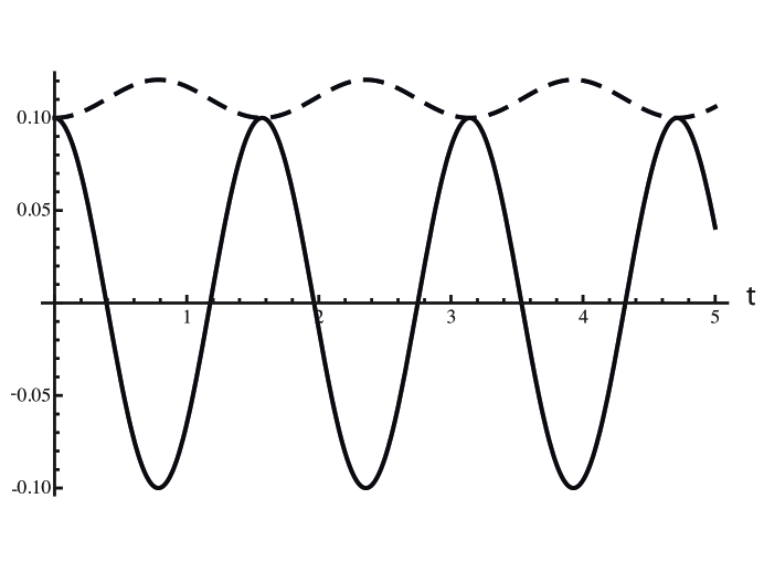
Figure 1: The figure illustrates that maximum negative energy density is obtained when we set $\omega=\Omega$ and $\delta=\pi$. The dotted line represents the Lorentz factor in Eq. (21), $[1-A^{2}\sin^{2}(\Omega\,t)]^{-1/2}$, while the solid line represents the cosine term, $-\cos(2\,\Omega\,t-\delta)=\cos(2\,\Omega\,t)$ both graphed as functions of time. Here we have chosen $A=0.2$ and $\Omega=2$. (The figures have been appropriately scaled to allow easier visualization.)

In this case, the integrated energy density becomes

$$I=\frac{r\,\Omega}{V}\int\frac{dt}{\sqrt{1-A^{2}{\rm sin}^{2}(\Omega t)}}\,{\rm cos}(2\,\Omega\,t)\,.$$ (22)

If we perform the integration on $t$ and multiply by the quantization volume, we get

$$I\,V\approx\frac{r\,[2\,E(\Omega\,t,A^{2})+(A^{2}-2)\,F(\Omega\,t,A^{2})}{A^{2}}\,,$$ (23)

where $F(\Omega\,t,A^{2})$ and $E(\Omega\,t,A^{2})$ are elliptic integrals of the first and second kind, respectively.

As a specific example, let us plot $I\,V$ for $r=0.01$, $A=0.9$, and in units where $\Omega=1$. Since, strictly speaking, the energy density is inversely proportional to $V$, we want to make a graph of $I\,V$ as a function of $\tau$, i.e., a graph of the integrated energy density, multiplied by the quantization volume, seen by the accelerated observer as a function of his proper time. The relation between $\tau$ and $t$ is $\tau=\int dt/\gamma$, which is

$$\tau=\frac{E(\Omega\,t,A^{2})}{\Omega}\,.$$ (24)

If we plot Eq. (23) against Eq. (24) for our chosen parameters, we get Fig. 2.

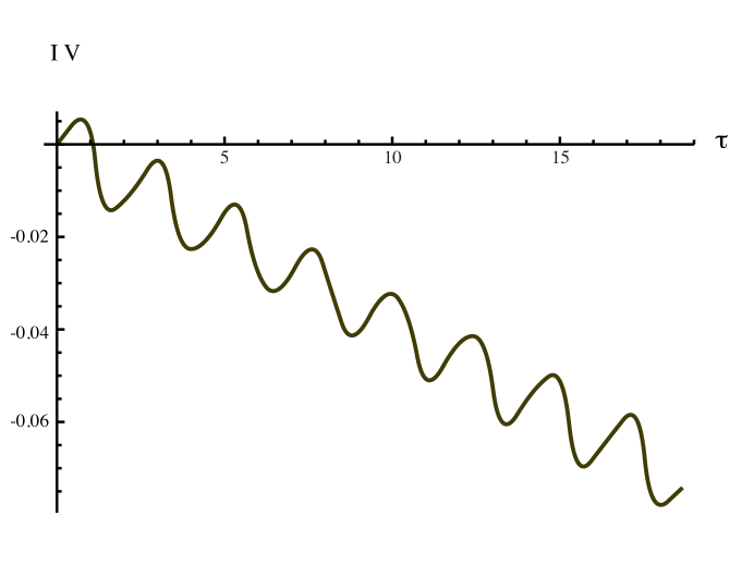
Figure 2: The integrated energy density multiplied by the quantization volume, $I\,V$, seen by an accelerated observer who is moving perpendicularly to the direction of wave propagation, is plotted as a function of his proper time, $\tau$, for the parameters $r=0.01$, $A=0.9$, and in units where $\Omega=1$.

Now let us examine our expression for $I$ in the $A\ll 1$ limit. If we expand the Lorentz factor to second-order in $A$, we obtain

$$\frac{1}{\sqrt{1-A^{2}{\rm sin}^{2}(\Omega t)}}\approx 1+\frac{1}{2}A^{2}{\rm sin}^{2}(\Omega\,t)+{\mathcal{O}}(A^{4})\,.$$ (25)

In this limit, the difference between $dt$ and $d\tau$ will be ${\mathcal{O}}(A^{2})$. If we use Eq. (25) in Eq. (22) to calculate $I$, we find:

$$I\approx-\frac{rA^{2}\,\Omega\,T}{8V}+\frac{r\,{\rm sin}(2\,\Omega\,T)}{2V}+\frac{r\,A^{2}{\rm sin}(2\,\Omega\,T)}{8V}-\frac{r\,A^{2}{\rm sin}(4\,\Omega\,T)}{32V}\,.$$ (26)

The sinusoidal terms will eventually be dominated by the linear term, but this can take many cycles, so we keep the ${\mathcal{O}}(A^{0})$ sinusoidal term, but drop the ${\mathcal{O}}(A^{2})$ sinusoidal terms. Therefore, our two leading order terms are

$$I\approx-\frac{rA^{2}\,\Omega\,T}{8V}+\frac{r\,{\rm sin}(2\,\Omega\,T)}{2V}\,.$$ (27)

Here $A^{2}\ll 1$, so the oscillating term is larger in magnitude until $T>4/(A^{2}\,\Omega)$. After this, the linear term dominates. However, we should recall that there is positive $r^{2}$ term in Eq. (15). This term will give a contribution to $I$ of $\Omega\,r^{2}\,T/V$, and is negligible only if we require that

$$8\,r\ll A^{2}\,.$$ (28)

Nonetheless, accumulating negative energy density, can occur for arbitrarily small velocities. For any $A\not=0$, we can find a value of $r$ which satisfies Eq. (28). Then eventually the first term in Eq. (27) will dominate.

II.2 Parallel Motion

We now consider the case of the accelerating observer moving parallel to the direction of the propagation of the wave. In the lab frame, we have $\langle T^{tt}\rangle=\langle T^{zz}\rangle=\langle T^{tz}\rangle$. The accelerated observer’s three-velocity and position, respectively, are

$$v = v^{z}(t)=\frac{dz}{dt}=A\,{\rm sin}(\omega\,t)\,,$$ (29)

$$z(t) = -\frac{A}{\omega}\,{\rm cos}(\omega\,t)$$ (30)

and so

$$u^{\mu}=\gamma(1,0,0,v)\,,$$ (31)

where $u^{t}=\gamma={dt}/{d\tau}$. Therefore, we have that

$$\langle T^{t^{\prime}t^{\prime}}\rangle=\gamma^{2}\,\Bigl{(}1-2v+v^{2}\Bigr{)}\,\langle T^{tt}\rangle=\Biggl{(}\frac{1-v}{1+v}\Biggr{)}\,\langle T^{tt}\rangle\,$$ (32)

where $(1-v)/(1+v)$ is a linear Doppler shift factor (as opposed to the transverse Doppler factor in the perpendicular case). As a result,

$$I=\int\langle T^{\mu\nu}\rangle u_{\mu}u_{\nu}d\tau=\int\Biggl{(}\frac{1-v}{1+v}\Biggr{)}\,\langle T^{tt}\rangle\,d\tau=\int\frac{\,\,(1-v)^{3/2}}{\sqrt{1+v}}\,\langle T^{tt}\rangle\,dt\,,$$ (33)

since $d\tau=\gamma^{-1}dt=\sqrt{1-v^{2}}dt$.

Here the observer is moving in the direction of wave propagation, so we can no longer set $z=0$. Now the energy density in the inertial frame is given by Eq. (12), with $z=-(A/\omega)\,{\rm cos}(\omega\,t)$, so

$$\langle T^{tt}\rangle=\frac{\Omega}{V}\,\sinh r\,\left\{\sinh r-\cosh r\,\cos\left[\left(\frac{2A\Omega}{\omega}\right)\cos(\omega t)+2\Omega t-\delta\right]\right\}\,.$$ (34)

In this case, we find accumulating negative energy density for $\omega=2\,\Omega$, and $\delta=-\pi/2$. The integral in Eq. (33) can be done analytically for small $A$, as will be discussed below, but for more general $A$, it can only be performed numerically. As an example, let us choose the case where $r=0.01$, $\delta=-\pi/2$, $A=0.9$, and $\omega=2$, in units where $\Omega=1$. In Fig. 3, we graph $IV$ against the observer’s proper time, which will again be given by Eq. (24).

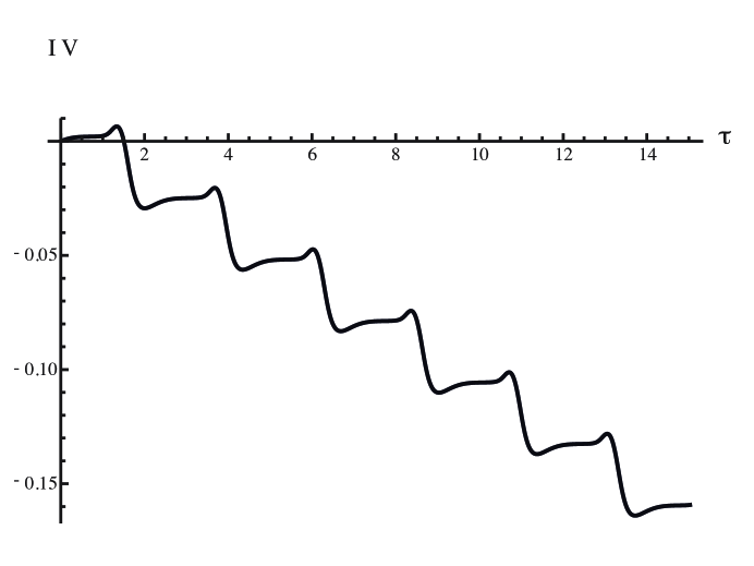
Figure 3: The integrated energy density multiplied by the quantization volume, $I\,V$, seen by an accelerated observer who is moving parallel to the direction of wave propagation, is plotted as a function of his proper time, $\tau$, for the parameters $r=0.01$, $A=0.9$, and $\omega=2$, in units where $\Omega=1$. Note that the accumulated negative energy density grows much faster than in the case of the perpendicularly moving observer, due to the linear Doppler shift term in the energy density. We also see extra structure in this curve as well, because the expression for the energy density is more complicated than in the perpendicular motion case.

Now we wish to consider the non-relativistic limit, and work to first order in $v$ and hence in $A$. To this order, $d\tau\approx dt$, so

$$I\approx\int\langle T^{t^{\prime}t^{\prime}}\rangle\,dt\,,$$ (35)

where the energy density in the accelerating frame is

$$\langle T^{t^{\prime}t^{\prime}}\rangle\approx(1-2v)\,\langle T^{tt}\rangle\,.$$ (36)

If we expand Eq. (34) to first order in $A$, the result is

$$\langle T^{tt}\rangle\approx\frac{\Omega}{V}\,\sinh r\,\left\{\sinh r-\cosh r\,\left[\cos(2\Omega t-\delta)-\frac{2\Omega}{\omega}\,A\,\cos(\omega t)\,\sin(2\Omega t-\delta)\right]\right\}\,,$$ (37)

where we have used the fact that

$$\cos\Biggl{[}\Biggl{(}\frac{2\Omega\,A}{\omega}\Biggr{)}\,\cos(\omega t)\Biggr{]} \approx 1+O(A^{2})\,,$$

$$\sin\Biggl{[}\Biggl{(}\frac{2\Omega\,A}{\omega}\Biggr{)}\,\cos(\omega t)\Biggr{]} \approx \Biggl{(}\frac{2\Omega\,A}{\omega}\Biggr{)}\,\cos(\omega t)+O(A^{3})\,.$$ (38)

Next we evaluate the energy density in the accelerating frame to first order in $A$ and set $\omega=2\Omega$ to find

$$\langle T^{t^{\prime}t^{\prime}}\rangle \approx \frac{\Omega}{V}\,\sinh r\,\left\{\sinh r\,\left[1-2A\sin(2\Omega t)\right]\right.$$ (39)

$$- \left.\cosh r\,\left[\cos(2\Omega t-\delta)-\frac{3}{2}A\sin(4\Omega t-\delta)-\frac{1}{2}\,A\,\sin\delta\right]\right\}\,.$$

This expression reveals that we can have growing negative energy density if $\delta=-\pi/2$ and $r\ll 1$. In this case, we may write

$$\langle T^{t^{\prime}t^{\prime}}\rangle\approx\frac{\Omega}{V}\,\left[r^{2}-r\left(\frac{1}{2}\,A-\sin(2\Omega t)\right)\right]\,,$$ (40)

where order $A$ oscillatory terms have been dropped. If

$$r\ll\frac{1}{2}\,A\,,$$ (41)

which is the analog of Eq. (28), the integrated energy density grows negatively as

$$I\approx-\frac{r\,A\,\Omega\,T}{2V}+\frac{r}{2V}[1-\cos(2\Omega T)]\sim-\frac{r\,A\,\Omega\,T}{2V}\,.$$ (42)

The latter asymptotic form holds for

$$T\gg\frac{1}{\Omega\,A}\,.$$ (43)

In the parallel motion case, the rate of growth of the negative integrated energy density is first order in $A$, as compared to second order in the perpendicular motion case treated in the previous subsection. This is due to the fact that in the parallel case, there is a linear Doppler shift, whereas in the perpendicular case the Doppler shift is transverse.

III Oscillations in a Cavity

III.1 The Perpendicular Case

We now consider the case of a particle oscillating in a closed cavity with dimensions $a$, $b$, and $d$ aligned along the $x$, $y$, $z$ axes respectively, where $b<a<d$. The modes in this cavity were discussed in Ref. FR09 . With the condition that $b<a<d$, the lowest frequency mode is the TE mode with $p=l=1,m=0$, where the frequency of the mode is given by

$$\Omega=\pi\sqrt{\frac{1}{a^{2}}+\frac{1}{d^{2}}}\,,$$ (44)

and the non-zero components of the electric and magnetic fields are

$${\cal E}_{x} = {\cal E}_{z}=0\,,$$

$${\cal E}_{y} = \frac{\Omega a}{\pi}\,C\,\sin\Big{(}\frac{\pi}{a}x\Big{)}\,\sin\Big{(}\frac{\pi}{d}z\Big{)}\,e^{-i\,\Omega\,t}\,,$$

$${\cal B}_{x} = i\,\,\frac{a}{d}\,\,C\,\sin\Big{(}\frac{\pi}{a}x\Big{)}\,\cos\Big{(}\frac{\pi}{d}z\Big{)}\,e^{-i\,\Omega\,t}\,,$$

$${\cal B}_{y} = 0\,,$$

$${\cal B}_{z} = -i\,C\,\cos\Big{(}\frac{\pi}{a}x\Big{)}\,\sin\Big{(}\frac{\pi}{d}z\Big{)}\,e^{-i\,\Omega\,t}\,,$$ (45)

where the electric field is taken to be polarized in the $y$-direction. This mode is independent of $y$. Here $C$ is a real normalization constant, given by

$$C^{2}=\frac{2\,\Omega}{a\,b\,d\,(1+a^{2}/d^{2})}\,.$$ (46)

For the case where only a single mode $j$ is excited, the normal ordered expectation values of the squared fields are

$$\langle E^{2}\rangle=2\langle a^{\dagger}\,a\rangle\,|{\cal E}_{j}|^{2}+2Re\Big{(}\langle a^{2}\rangle\,{\cal E}_{j}^{2}\Big{)}$$ (47)

and

$$\langle B^{2}\rangle=2\langle a^{\dagger}\,a\rangle\,|{\cal B}_{j}|^{2}+2Re\Big{(}\langle a^{2}\rangle\,{\cal B}_{j}^{2}\Big{)}\,.$$ (48)

where

$${\cal E}_{j}^{2} = {{\cal E}_{y}}^{2}=\frac{\Omega^{2}a^{2}}{\pi^{2}}\,C^{2}\,{\rm sin}^{2}\Big{(}\frac{\pi}{a}x\Big{)}\,{\rm sin}^{2}\Big{(}\frac{\pi}{d}z\Big{)}\,e^{-2i\Omega t}$$

$${\cal B}_{j}^{2} = {\cal B}_{x}^{2}+{\cal B}_{z}^{2}=-C^{2}\Bigg{[}{\rm cos}^{2}\Big{(}\frac{\pi}{a}x\Big{)}\,{\rm sin}^{2}\Big{(}\frac{\pi}{d}z\Big{)}+\frac{a^{2}}{d^{2}}\,{\rm sin}^{2}\Big{(}\frac{\pi}{a}x\Big{)}\,{\rm cos}^{2}\Big{(}\frac{\pi}{d}z\Big{)}\Bigg{]}\,e^{-2i\Omega t}\,.$$ (49)

In this case, we can have the particle moving in the $y$-direction, and located in the center of the cavity in the other directions, so that

$$x=\frac{a}{2},\,z=\frac{d}{2}\,.$$ (50)

This considerably simplifies the mode functions, leading to

$${\cal B}_{x}={\cal B}_{z}=0\,,\qquad{\cal E}_{y}=\frac{\Omega\,a}{\pi}\,C\,{\rm e}^{-i\Omega t}\,.$$ (51)

The only non-zero components of the stress tensor which we will need are $\langle T^{tt}\rangle$ and $\langle T^{yy}\rangle$, which become

$$\langle T^{tt}\rangle = -\langle T^{yy}\rangle=\sinh r\left[\sinh r\,|{\cal E}_{y}|^{2}-\cosh r\,{\rm Re}\left({\rm e}^{i\delta}\,{\cal E}_{y}^{2}\right)\right]$$ (52)

$$= N\,\sinh r\left[\sinh r-\cosh r\,\cos(2\Omega t-\delta)\right]\,,$$

where

$$N=\left(\frac{\Omega\,a}{\pi}\,C\right)^{2}\,.$$ (53)

Because the direction of oscillation of the particle is in the $y$-direction,

$$u^{\mu}=\gamma(1,0,v^{y},0)\,,$$ (54)

where $v^{y}=A\,\sin\omega t$. The integrand of $I$ is

$$\langle T_{\mu\nu}u^{\mu}u^{\nu}\rangle d\tau=\frac{(\langle T_{tt}\rangle+({v^{y}})^{2}\langle T_{yy}\rangle)}{\sqrt{1-A^{2}{\rm sin}^{2}(\omega t)}}\,dt=\sqrt{1-A^{2}{\rm sin}^{2}(\omega t)}\,\langle T_{tt}\rangle\,dt\,.$$ (55)

Let

$$U=\sqrt{1-A^{2}{\rm sin}^{2}(\omega t)}\,\langle T_{tt}\rangle\,.$$ (56)

We will assume that $A\ll 1$, and expand to second order in $A$. Therefore, if we use Eq. (52) in Eq. (55), and set $\omega=\Omega$, we have that

$$U\approx N\,\Bigl{(}1-\frac{1}{2}\,A^{2}\sin^{2}(\Omega t)\Bigr{)}\,[\sinh^{2}r-\sinh r\,\cosh r\cos(2\Omega t-\delta)]\,.$$ (57)

If we now expand the right-hand side of Eq. (57) to second order in $r$, set $\delta=0$, integrate from $0$ to $T$, and drop oscillatory terms in $A^{2}$, we obtain

$$I\approx N\,\Biggl{(}r^{2}T-\frac{1}{8}\,A^{2}rT-r\,\frac{\sin(2\Omega T)}{2\,\Omega}\Biggr{)}\,,$$ (58)

where we have also dropped a higher order $A^{2}\,r^{2}$ term.

The positive first term is negligible compared to the second when

$$r\ll\frac{1}{8}\,A^{2}\,.$$ (59)

The middle negative linear growing term will dominate the sinusoidal term when

$$T>\frac{4}{A^{2}\,\Omega}$$ (60)

In this case, the restrictions on $r$ and $T$ are the same as those for perpendicular motion in the plane wave case. In these limits, we therefore have negative energy density which grows linearly as

$$I\approx-\frac{1}{8}\,N\,A^{2}rT\,.$$ (61)

If we use Eqs. (46) and (53), we can write the previous equation as

$$I\approx-\frac{r\,A^{2}\,\Omega\,T}{4V}\,,$$ (62)

where $V=abd$ is the volume of the cavity. Compare this result with the first term in Eq. (27), the corresponding rate for perpendicular motion in a plane wave mode. If we identify the cavity volume in the former with the quantization volume in the latter, then they differ only by a factor of two.

III.2 The Parallel Case

In this subsection, we will consider the case of a particle oscillating in a cavity along the $z$-axis, in the limit where $A\ll 1$, and work to first order in $A$. We take

$$v_{z}=A\,{\sin\,}\omega t\,,$$ (63)

and

$$z=z_{0}-\frac{A\,{\cos}\,\omega t}{\omega}+O(A^{2})\,,$$ (64)

where $z=z_{0}$ corresponds to the equilibrium position of the particle, and the last term corresponds to relativistic corrections. We will choose the $x$-position of the particle to be

$$x=\frac{a}{2}\,.$$ (65)

The energy density in the particle’s frame is

$$\langle T^{t^{\prime}t^{\prime}}\rangle=\gamma^{2}\,\langle(T^{tt}-2v_{z}\,T^{tz}+{v_{z}}^{2}\,T^{zz})\rangle\approx\langle T^{tt}\rangle-2v_{z}\,\langle T^{tz}\rangle\,.$$ (66)

Here

$$\langle T^{tz}\rangle=-\langle E_{y}\,B_{x}\rangle\,.$$ (67)

We need to calculate $\langle T^{tt}\rangle$ and $\langle T^{tz}\rangle$ using the mode functions in Eq. (45), and then expand the result to second order in $r$. The result for $\langle T^{t^{\prime}t^{\prime}}\rangle$ may be written as

$$\langle T^{t^{\prime}t^{\prime}}\rangle\approx C^{2}\,\{(F_{1}+2v_{z}\,F_{3})r^{2}-r\,[F_{2}\,\cos(2\Omega t-\delta)+2v_{z}\,F_{3}\,\sin(2\Omega t-\delta)]\}\,,$$ (68)

where

$$F_{1}=F_{1}(z)=\frac{\Omega^{2}\,a^{2}}{\pi^{2}}\,\Biggl{[}{\rm sin}^{2}\Biggl{(}\frac{\pi z}{d}\Biggr{)}+\frac{a^{2}}{d^{2}}\,{\rm cos}^{2}\Biggl{(}\frac{\pi z}{d}\Biggr{)}\Biggr{]}\,,$$ (69)

$$F_{2}=F_{2}(z)=\frac{\Omega^{2}\,a^{2}}{\pi^{2}}\,\Biggl{[}{\rm sin}^{2}\Biggl{(}\frac{\pi z}{d}\Biggr{)}-\frac{a^{2}}{d^{2}}\,{\rm cos}^{2}\Biggl{(}\frac{\pi z}{d}\Biggr{)}\Biggr{]}\,,$$ (70)

and

$$F_{3}=F_{3}(z)=\frac{\Omega\,a^{2}}{\pi d}\,{\rm sin}\Biggl{(}\frac{2\,\pi z}{d}\Biggr{)}\,,$$ (71)

and where $C^{2}$ is once again given by Eq. (46).

The integrated energy density may be written as

$$I\approx\int dt\,\langle T^{t^{\prime}t^{\prime}}\rangle\approx C^{2}\,(r^{2}\,I_{1}-r\,I_{2})$$ (72)

where

$$I_{1}=\int_{0}^{T}\,dt\,(F_{1}+2v_{z}\,F_{3})\,,$$ (73)

and

$$I_{2}=\int_{0}^{T}\,dt\,[F_{2}\,\cos(2\Omega t-\delta)+2v_{z}\,F_{3}\,\sin(2\Omega t-\delta)]\,.$$ (74)

As in the case of parallel motion in the plane wave case, with the appropriate choices for $\omega,\,\Omega,\,r$ and $\delta$, we expect to get a linearly growing negative term, a term which is first order in $r$ and sinusoidal in time, and a positive $r^{2}$ term. The first and second of these terms will arise from $F_{2}$ and $F_{3}$, while the third term will arise from $F_{1}$. We also expect that we will find a non-trivial effect in first order in $A$.

Let us first examine the terms involving $F_{3}$ in Eq. (68). These terms both involve the product $v_{z}\,F_{3}$, and are hence already of order $A$. Thus we may use Eq. (64) to write

$$F_{3}(z)\approx F_{3}(z_{0})=\frac{\Omega\,a^{2}}{\pi\,d}\,,$$ (75)

where we have set $z_{0}=d/4$. (As it turns out, the linearly growing term we want will come from the $F_{3}$ term in $I_{2}$, so we cannot choose $z_{0}=d/2$.)

A similar situation applies to $F_{1}$, which contributes only to an order $r^{2}$ term. This is a positive, growing term which we need only to zeroth order in $A$. For this purpose, we may evaluate $F_{1}$ at $z=z_{0}$:

$$F_{1}(z)\approx F_{1}(z_{0})=\frac{\Omega^{2}\,a^{2}}{2\pi^{2}}\,\left(1+\frac{a^{2}}{d^{2}}\right)\,.$$ (76)

Thus, for estimating the order $r^{2}$ term, we may use

$$I_{1}\sim F_{1}\,T\,,$$ (77)

where $F_{1}$ has the value in Eq. (76).

The negatively growing term comes from $I_{2}$, which involves $F_{2}$, so we need to expand the latter to first order in $A$, using Eq. (64), as

$$F_{2}(z) = \frac{\Omega^{2}\,a^{2}}{2\pi^{2}}\,\left[\left(1-\frac{a^{2}}{d^{2}}\right)-\left(1+\frac{a^{2}}{d^{2}}\right)\,\cos\left(\frac{2\pi z}{d}\right)\right]$$ (78)

$$\approx \frac{\Omega^{2}\,a^{2}}{2\pi^{2}}\,\left[\left(1-\frac{a^{2}}{d^{2}}\right)-\left(1+\frac{a^{2}}{d^{2}}\right)\,\left(\frac{2\pi A}{d\,\omega}\right)\,\cos(\omega t)\right]\,.$$

The $I_{2}$ term will be maximally negative when $\omega=2\,\Omega$ and $\delta=0$. In this case, a short calculation yields

$$I_{2}\approx A\,\frac{\Omega\,a^{2}}{4\pi d}\,\left(3-\frac{a^{2}}{d^{2}}\right)\,T+\frac{\Omega\,a^{2}}{4\pi}\,\left(1-\frac{a^{2}}{d^{2}}\right)\,\sin(2\Omega T)\,,$$ (79)

where oscillatory, order $A$ terms have been dropped. Note that $3-{a^{2}}/{d^{2}}>0$ because $a<d$.

Therefore, the integrated energy density becomes,

$$I\approx C^{2}\,\left[-r\,A\,T\,\frac{\Omega\,a^{2}}{4\pi d}\,\left(3-\frac{a^{2}}{d^{2}}\right)-\,r\,\frac{\Omega\,a^{2}}{4\pi^{2}}\,\left(1-\frac{a^{2}}{d^{2}}\right)\,\sin(2\Omega T)+r^{2}\,T\,\frac{\Omega^{2}\,a^{2}}{2\pi^{2}}\,\left(1+\frac{a^{2}}{d^{2}}\right)\right]\,.$$ (80)

We see that the negative linearly growing term will dominate the sinusoidal term when

$$T>\frac{d}{\pi A}\,\left(\frac{d^{2}-a^{2}}{3d^{2}-a^{2}}\right)\,.$$ (81)

and the positive, order $r^{2}$ term, when

$$\frac{2\Omega d}{\pi}\,\left(\frac{d^{2}+a^{2}}{3d^{2}-a^{2}}\right)\,r<A\,.$$ (82)

In this case, we find that the integrated energy density in the particle’s frame grows negatively as

$$I\sim-\frac{rA\Omega}{2V}\,T\;\left[\frac{\Omega\,a^{2}}{\pi d}\,\Biggl{(}\frac{3d^{2}-a^{2}}{d^{2}+a^{2}}\Biggr{)}\right]\,,$$ (83)

where we have used the definition of $C^{2}$ and the fact that $V=abd$ is the volume of the cavity. Compare this result with Eq. (42), the corresponding rate for parallel motion in a plane wave mode. If we identify the cavity volume in the former with the quantization volume in the latter, then they differ only by the factor in the square brackets. If $a$ and $d$ are of the same order of magnitude, then Eq. (44) tells us that $\Omega\sim O(1/a)\sim O(1/d)$, and this factor is of order unity.

IV Effects of the Negative Energy on Focussing

In this section, we will treat one possible effect of the accumulating negative energy along a particle’s worldline. It is well-known that the attractive character of gravity, with ordinary matter as a source, leads to focussing of null and timelike geodesics. One expects that negative energy densities might have the opposite effect, and produce defocussing through repulsive gravitational effects.

IV.1 Raychaudhuri Equation

The effect of gravity on a congruence of timelike worldlines is described by the Raychaudhuri equation. In our case, we allow the worldlines to be non-geodesics, so the equation takes the form HE

$${\dot{\theta}}=\frac{d\theta}{d\tau}=-R_{\alpha\beta}u^{\alpha}u^{\beta}+2\omega_{\alpha\beta}\omega^{\alpha\beta}-2\sigma_{\alpha\beta}\sigma^{\alpha\beta}-\frac{1}{3}\theta^{2}+\nabla_{\beta}a^{\beta}\,.$$ (84)

Here $u^{\alpha}$ and $a^{\beta}=u^{\alpha}\nabla_{\alpha}u^{\beta}$ are the 4-velocity and 4-acceleration of the congruence, and $\sigma_{\alpha\beta}$ and $\omega_{\alpha\beta}$ are the shear and vorticity tensors. Also, $\theta=\nabla_{\alpha}u^{\alpha}$ is the expansion, and $R_{\alpha\beta}$ is the Ricci tensor. The last term in Eq. (84) is the acceleration term, which vanishes for geodesics. We will assume a hypersurface orthogonal congruence, in which case the vorticity tensor vanishes, $\omega_{\alpha\beta}=0$. In addition, we assume that the shear and expansion are sufficiently small, that the terms quadratic in those quantities may be neglected. In this case, the Raychaudhuri equation becomes

$${\dot{\theta}}\approx-R_{\alpha\beta}u^{\alpha}u^{\beta}+{\dot{\theta}}_{\rm ac}\,,$$ (85)

where ${\dot{\theta}}_{\rm ac}=\nabla_{\beta}a^{\beta}$ is the acceleration term, and the Ricci tensor term describes the effects of gravity.

Next we assume that an electromagnetic field is both the cause of the acceleration and the sole source of the gravitational field. Particles with rest mass $m$ and electric charge $q$ obey the equation of motion

$$a_{\beta}=\frac{q}{m}\,F_{\beta\rho}\,u^{\rho}\,,$$ (86)

where the field strength tensor, $F_{\beta\rho}$, is assumed to obey the source free equation

$$\nabla_{\alpha}\,F^{\alpha\beta}=0\,.$$ (87)

We can now write the acceleration term as

$${\dot{\theta}}_{\rm ac}=\frac{q}{m}F^{\alpha\beta}(\nabla_{\alpha}u_{\beta})\,.$$ (88)

The covariant derivative of the 4-velocity may be expressed as MTW

$$\nabla_{\alpha}u_{\beta}=\sigma_{\beta\alpha}+\frac{1}{2}\theta(g_{\alpha\beta}+u_{\alpha}u_{\beta})-a_{\beta}u_{\alpha}\,,$$ (89)

when $\omega_{\beta\alpha}=0$. However, all terms on right hand side of this expression, except for the last, are symmetric tensors which vanish when contracted into the antisymmetric field strength tensor. Thus we obtain

$${\dot{\theta}}_{\rm ac}=-a_{\beta}a^{\beta}\,.$$ (90)

The electromagnetic stress tensor, given in Eq. (3) is tracefree, so the Einstein equations become

$$R_{\alpha\beta}=8\pi{\ell_{p}}^{2}\,T_{\alpha\beta}\,,$$ (91)

where $\ell_{p}$ is the Planck length, and Newton’s constant is $G={\ell_{p}}^{2}$, in units where $\hbar=c=1$. We may write

$$T_{\alpha\beta}u^{\alpha}u^{\beta}=(u^{\alpha}F_{\alpha\rho})u^{\beta}{F_{\beta}}^{\rho}+\frac{1}{4}F_{\mu\nu}F^{\mu\nu}=\frac{m^{2}}{q^{2}}\,a_{\rho}a^{\rho}+\frac{1}{4}F_{\mu\nu}F^{\mu\nu}\,,$$ (92)

where we have used Eq. (86). We may use this expression to evaluate the Ricci tensor term in the Raychaudhuri equation and write

$${\dot{\theta}}\approx-\Biggl{(}1+8\pi\frac{{\ell_{p}}^{2}\,m^{2}}{q^{2}}\Biggr{)}\,a_{\rho}a^{\rho}-2\pi{\ell_{p}}^{2}\,F_{\mu\nu}F^{\mu\nu}\,.$$ (93)

IV.2 Fields Producing Acceleration

In previous sections, we assumed a prescribed sinusoidal motion, but did not explicitly give the electromagnetic fields which would produce this motion. Here we will concentrate on the case of motion parallel to a plane wave mode, which was treated in Sec. II.2. In particular, we consider the case of non-relativistic motion along the $z$-direction, as described by Eq. (29), with $A\ll 1$. This motion can approximately be produced by a plane wave with polarization in the $z$-direction. Here we will consider a classical electromagnetic wave propagating in the $y$-direction, with electric field ${\bf E}=E_{c}\,{\bf\hat{z}}$, and magnetic field ${\bf B}=E_{c}\,{\bf\hat{x}}$, where

$$E_{c}=\frac{\omega\,A\,m}{q}\;\cos\omega(t-y)\,.$$ (94)

To order $A$, only the electric field determines the motion of the particle, with the magnetic force contributing in order $A^{2}$. Because the motion of the particle is only in the $z$-direction, we may set $y=0$. In this case, the energy density of the classical wave, in the laboratory frame, is

$$T_{c}^{tt}=E_{c}^{2}=\left(\frac{\omega\,A\,m}{q}\right)^{2}\;\cos^{2}(\omega t)\,.$$ (95)

In addition to this classical field, the particle is also subjected to the quantum fields associated with the squeezed vacuum state mode. These fields potentially produce a fluctuating force on the particle, which we wish to include. Let $\mathbf{E}_{q}$ and $\mathbf{B}_{q}$ be the terms in Eqs. (7) and (8), respectively, which refer to the mode in a squeezed vacuum state. That is,

$$\mathbf{E}_{q}=\hat{\bf x}\,({\mathcal{E}}\,a+{\mathcal{E}}^{\ast}\,a^{\dagger})\,,$$ (96)

and

$$\mathbf{B}_{q}=\hat{\bf y}\,({\mathcal{E}}\,a+{\mathcal{E}}^{\ast}\,a^{\dagger})\,,$$ (97)

where ${\mathcal{E}}$ is defined in Eq. (9). We will treat the velocity of the particle due to the quantum electric field as an operator in the photon state space, $\mathbf{v}_{q}=v_{q}\,\hat{\bf x}$, where $v_{q}$ will be evaluated explicitly below.

There is a third effect which we will not include explicitly. This the effect of the emitted radiation by the particle. There will be an average radiation reaction force which will slightly change the trajectory of the particle for a given classical field. However, this is normally very small and will be neglected. There will also be a shot noise effect, an uncertainty in the particle’s momentum due to the statistical uncertainty in the number of photons emitted. This effect depends primarily on the classical field driving the average motion and not upon the quantum electric field. Hence it, and the radiation reaction force, would cancel in any experiment which compares particle motion with and without the quantum electric field. In addition, this momentum uncertainty grows as the square root of the mean number of photons radiated, and hence as the square root of time. Here we are interested in effects which grow linearly in time.

We will now compute the components of the acceleration four-vector in the lab rest frame, taking account of both the classical and quantum parts of the electromagnetic field and of the particle’s four-velocity. The acceleration four-vector satisfies

$$a^{\rho}=\frac{q}{m}\,F^{\rho\alpha}\,u_{\alpha}\,.$$ (98)

In the non-relativisitic limit, the four-velocity is

$$u^{\alpha}=(1,v_{q},0,v_{c})\,,$$ (99)

where $v_{c}=A\,\sin(\omega t)$ . The non-zero components of the field strength tensor are

$$F^{tz}=F^{yz}=E_{c}\qquad F^{tx}=F^{zx}=E_{q}\,,$$ (100)

and those obtained by antisymmetry of $F^{\rho\alpha}$. The components of $a^{\rho}$ become

$$a^{t} = \frac{q}{m}\,(E_{q}\,v_{q}+E_{c}\,v_{c})$$

$$a^{x} = \frac{q}{m}\,E_{q}\,(1-v_{c})$$

$$a^{y} = \frac{q}{m}\,E_{c}\,v_{c}$$

$$a^{z} = \frac{q}{m}\,(E_{q}\,v_{q}+E_{c})\,.$$ (101)

We can now form the scalar $a^{\rho}a_{\rho}$, expand it to first order in the velocities, dropping $v_{c}^{2}$, $v_{q}^{2}$ and $v_{c}v_{q}$ terms, and take its expectation value in the squeezed vacuum state. The result is

$$\langle a^{\rho}a_{\rho}\rangle\approx\frac{q^{2}}{m^{2}}\,\left[\langle E_{q}^{2}\rangle(1-2v_{c})+E_{c}^{2}+2E_{c}\langle E_{q}v_{q}\rangle\right]\,.$$ (102)

Let us examine each term on the right-hand side of this expression. The classical energy density, which is the same to first order in velocity in the lab frame and in the particle rest frame, is just $E_{c}^{2}$. Because the classical wave is propagating in the $y$-direction, and all the motion is in the $x$ and $z$ directions, this is the perpendicular motion case, with respect to the classical wave. Thus, to order $v$, $T_{c}^{t^{\prime}t^{\prime}}\approx T_{c}^{tt}$, since $T_{c}^{t^{\prime}t^{\prime}}\approx T_{c}^{tt}+O(v^{2})$. The expectation value of the quantum energy density in the lab frame is $\langle E_{q}^{2}\rangle$, and is given explicitly by Eq. (12). This quantity in the particle rest frame is $\langle E_{q}^{2}\rangle(1-2v_{c})$. The final term is the contribution of the velocity fluctuations to the acceleration.

For both the classical and quantum electromagnetic fields, we have assumed plane waves, for which $E^{2}=B^{2}$, and hence $F_{\mu\nu}F^{\mu\nu}=0$. Thus we may drop the last term in Eq. (93), and write mean rate of change of the expansion as

$$\langle{\dot{\theta}}\rangle\approx-\Biggl{(}1+8\pi\frac{{\ell_{p}}^{2}\,m^{2}}{q^{2}}\Biggr{)}\,\langle a_{\rho}a^{\rho}\rangle\,.$$ (103)

IV.3 Velocity Fluctuations and Defocussing

The fluctuating part of the velocity, $v_{q}$, is determined by Eq. (101):

$$\frac{dv_{q}}{dt}=a^{x}=\frac{q}{m}\,E_{q}\,(1-v_{c})\,,$$ (104)

where the term proportional to $v_{c}$ on the right hand side is due to the magnetic force produced by $B_{y}$. Note that time derivative here is a total derivative, and we need to account for both the explicit time dependence and the implicit dependence through $z(t)$:

$$\frac{dv_{q}}{dt}=\frac{\partial v_{q}}{\partial t}+\frac{\partial v_{q}}{\partial z}\,v_{c}\,,$$ (105)

recalling that $v_{c}=dz/dt$. The solution to Eq. (104) becomes

$${v}_{q}=\frac{iq}{m\Omega}\,({\mathcal{E}}\,a-{\mathcal{E}}^{\ast}\,a^{\dagger})\,,$$ (106)

where we have used Eqs. (9) and (96). Note that the effects of the magnetic force and of the implicit time dependence cancel one another.

We may compute $\langle E_{q}v_{q}\rangle=\langle:E_{q}v_{q}:\rangle$ in a squeezed vacuum state to find

$$\langle E_{q}v_{q}\rangle=\frac{q}{mV}\,\sinh r\,\cosh r\,\sin[2\Omega(z-t)+\delta]\,.$$ (107)

Here we used

$$\langle a^{2}\rangle=\langle(a^{\dagger})^{2}\rangle^{\ast}=-{\rm e}^{i\delta}\,\sinh r\,\cosh r$$ (108)

in the squeezed vacuum state. We may use Eq. (94) with $y=0$, and set $\delta=-\pi/2$ to write

$$2E_{c}\,\langle E_{q}v_{q}\rangle=-\frac{2\omega\,A}{V}\,\sinh r\,\cosh r\,\cos(\omega t)\,\cos[2\Omega(z-t)]\,.$$ (109)

We will work only to first order in $A$, which means that we can ignore the $z$-dependence (see Eqs. (30) and  (38)) in the above expression, which will contribute in order $A^{2}$. When we set $\omega=2\Omega$, and drop oscillatory terms, then we have

$$2E_{c}\,\langle E_{q}v_{q}\rangle\approx-\frac{2\Omega\,A}{V}\,\sinh r\,\cosh r\,.$$ (110)

In the small $r$ limit, this becomes

$$2E_{c}\,\langle E_{q}v_{q}\rangle\approx-\frac{2\Omega\,A}{V}\,r\,,$$ (111)

which is to be compared with the same limit for the squeezed state energy density in the accelerated frame,

$$\langle E_{q}^{2}\rangle(1-2v_{c})\approx-\frac{\Omega\,A}{2V}\,r\,.$$ (112)

The latter quantity is just the order $r$, non-oscillatory term in Eq. (40). We see that both terms have the same form and same sign, and both contribute to defocussing, although the effect of the quantum velocity fluctuations is four times that of the negative energy density in this limit.

If we combine these terms, as well as the time average of the classical energy density, Eq. (95), evaluated at $\omega=2\Omega$, then Eq. (102) for the mean squared acceleration becomes

$$\langle a^{\rho}a_{\rho}\rangle\approx 2\,\Omega^{2}\,A^{2}-\frac{5q^{2}\,\Omega\,A\,r}{4Vm^{2}}\,\,.$$ (113)

The positive term is the focussing effect of the classical energy density, and the negative term is the combined defocussing effect of the negative energy density and the velocity fluctuations. These two terms depend upon different combinations of parameters, and it seems possible to arrange for the defocussing effect to dominate. Note that the gravitational effect, from the Ricci tensor, is $\propto{\ell_{p}}^{2}$ in Eq. (103). The part without ${\ell_{p}}^{2}$ is a pure acceleration effect from the acceleration term. However, both effects have the same functional form here.

V Summary and Discussion

The key result of this paper is that an accelerated observer undergoing sinusoidal motion in space can observe an average constant negative energy density, so the integrated energy density grows negatively in time in this observer’s frame. This is contrast to an inertial observer, in whose frame the energy density is more constrained by quantum inequalities. We considered a squeezed vacuum state for both a plane wave and a standing wave in a cavity. The case in which growing integrated negative energy is possible is when the squeeze parameter is small, $r\ll 1$. In this case, the energy density in an inertial frame is almost sinusoidal, with the positive energy outweighing the negative energy only in order $r^{2}$. The effect of the periodic motion of the accelerated observer is to introduce Doppler shift factors which enhance the negative energy compared to the positive energy. The accelerated observer then sees the negative energy blueshifted and the positive energy redshifted. In the cases of perpendicular motion treated in Sect. II.1 and III.1, the effect is a transverse Doppler shift, and is hence of order $A^{2}$, where $A$ is the oscillation amplitude. For the parallel motion cases in Sects. II.2 and III.2, the effect is a linear Doppler shift, leading to an effect of order $A$. It is possible to have growing negative integrated energy density even for arbitrarily slow motion, which means arbitrarily small $A$. However, for a given $A$, the squeeze state parameter $r$ is constrained by relations such as Eqs. (28) and (41), which limit the rate of growth. Note that non-relativistic motion is not a requirement for growing negative energy, and the numerically integrated results depicted in Figs. 1 and 3 are for relativistic motion, but small squeeze parameter.

We studied a model which gives an operational meaning to integrated negative energy density in the form of defocussing of bundle of worldlines. In Sect. IV, we analyzed the Raychaudhuri equation for the expansion along a bundle of accelerated worldlines. The motivation for this study is that positive energy leads to attractive gravitational effects and hence focussing, so negative energy should do the opposite. This expectation was born out in our results. However, the situation is complicated by the need to include an acceleration term in the Raychaudhuri equation, and the effects of the fluctuating velocity of the accelerating charged particles in a fluctuating electromagnetic field. In the cases which we examined, the gravitational effects and the acceleration effects have the same functional form.

The effect treated in this paper bears a superficial resemblance to the effect treated in Ref. PF11 , which is a linearly growing or decreasing mean squared velocity of a charged particle undergoing sinusoidal motion near a mirror. The latter effect can be interpreted as non-cancellation of anti-correlated quantum electric field fluctuations. A charge at rest in the Casimir vacuum produced by the mirror is subjected to field fluctuations which can give or take energy from the charge for a time consistent with the energy-time uncertainty principle, but this effect will be cancelled by a subsequent anti-correlated fluctuation. The sinusoidal motion upsets this cancellation, and allows the mean squared velocity to grow or decrease, depending upon the phase of the oscillation. The effect discussed in the present paper also involves linear growth, but does not have an obvious interpretation in terms of non-cancelling fluctuations. The natural interpretation seems to be in terms of Doppler shifts which can be arranged to enhance negative energy and suppress positive energy. A topic for future research is to study further the connection between these two effects.

Another topic is to understand to relation between the growing integrated negative energy and the general worldline quantum inequality of Fewster Fewster00 . This inequality is difficult to evaluate explicitly for the sinusoidal worldline considered here. In this case, the inequality must be weak enough to allow the linear growth found here, but it might provide insight into the allowed behavior in situations more general than we have treated.

A further question of interest is the possible physical consequences of accumulating negative energy beyond those discussed in Sect. IV. A possible detection model for negative energy was proposed in Ref. FR09 , in which negative energy can suppress the decay rate of atoms in excited states. The atoms in this model are moving along inertial worldlines, but it might be possible to devise a more general model involving non-inertial motion.

Let us also stress that our results do not in any way invalidate or diminish the implications of the quantum inequality bounds for inertial observers. The strength of a quantum inequality bound may depend on the particular observer chosen, but the validity of the bound does not. As an example, suppose one is using a quantum inequality, applied to the motion of a particular inertial observer, to determine constraints on the geometry of a traversable wormhole. Let us further assume that in this case, the quantum inequality provides a very strong constraint. Now suppose one looks at the same problem from the point of view of, say, a different inertial or an accelerating observer and finds a much weaker bound. The weakness of the latter bound does not invalidate the strength of the previous bound. The observer whose motion provides the strongest quantum inequality bound implies the strongest constraint on the geometry of the wormhole. The latter cases simply yield true but weaker bounds.

- (1) L.H. Ford, Int. J. Mod. Phys. A 25, 2355 (2010), arXiv:0911.3597.
- (2) L.H. Ford, Proc. R. Soc. London A364, 227 (1978).
- (3) L.H. Ford, Phys. Rev. D 43, 3972 (1991).
- (4) L.H. Ford and T.A. Roman, Phys. Rev. D 51, 4277 (1995), gr-qc/9410043.
- (5) L.H. Ford and T.A. Roman, Phys. Rev. D 55, 2082 (1997), gr-qc/9607003.
- (6) E.E. Flanagan, Phys. Rev. D 56, 4922 (1997), gr-qc/9706006.
- (7) C.J. Fewster and S.P. Eveson, Phys. Rev. D 58, 084010 (1998), gr-qc/9805024.
- (8) M.J. Pfenning, Phys. Rev. D 65, 024009, (2002), gr-qc/0107075.
- (9) C.J. Fewster and S. Hollands, Rev. Math. Phys. 17, 577 (2005), math-ph/0412028.
- (10) L.H. Ford, A. D. Helfer, and T. A. Roman, Phys. Rev. D 66, 124012 (2002), gr-qc/0208045.
- (11) L.H. Ford and T.A. Roman, Phys. Rev. D 53, 5496 (1996), gr-qc/9510071.
- (12) M.J. Pfenning and L.H. Ford, Class. Quant. Grav. 14, 1743 (1997), gr-qc/9702026.
- (13) C.J. Fewster, Class. Quantum Grav. 17, 1897 (2000).
- (14) S.A. Fulling and P.C.W. Davies, Proc. R. Soc. London A348, 393 (1976).
- (15) P.C.W. Davies and S.A. Fulling, Proc. R. Soc. London A356, 237 (1977).
- (16) C.J. Fewster and M.J. Pfenning, J. Math. Phys. 44, 082303 (2006), math-ph/0602042.
- (17) L.H. Ford and T.A. Roman, Annals Phys. 326, 2294 ( 2011), arXiv:0907.1638,
- (18) S.W. Hawking and G.F.R. Ellis, The Large Scale Structure of Space-time (Cambridge, 1973), p. 84, Eq. (4.26).
- (19) C.W. Misner, K.S. Thorne, and J.A. Wheeler, Gravitation, (Freeman, 1973), p. 566, Eq. (22.15a).
- (20) V. Parkinson and L.H. Ford, Phys. Rev. A 84, 062102 (2011), arXiv:1106.6334.