A Scaler-Based Data Acquisition System for Measuring Parity-Violating Asymmetry in Deep Inelastic Scattering

Abstract

An experiment that measured the parity-violating asymmetries in deep inelastic scattering was completed at the Thomas Jefferson National Accelerator Facility in experimental Hall A. From these asymmetries, a combination of the quark weak axial charge could be extracted with a factor of five improvement in precision over world data. To achieve this, asymmetries at the $10^{-4}$ level needed to be measured at event rates up to 600 kHz and the high pion background typical to deep inelastic scattering experiments needed to be rejected efficiently. A specialized data acquisition (DAQ) system with intrinsic particle identification (PID) was successfully developed and used: The pion contamination in the electron samples was controlled at the order of $2\times 10^{-4}$ or below with an electron efficiency of higher than 91% during most of the production period of the experiment, the systematic uncertainty in the measured asymmetry due to DAQ deadtime was below 0.5%, and the statistical quality of the asymmetry measurement agreed with the Gaussian distribution to over five orders of magnitudes. The DAQ system is presented here with an emphasis on its design scheme, the achieved PID performance, deadtime effect and the capability of measuring small asymmetries.

, , , , , , , ,

1 Introduction

The Parity-Violating Deep Inelastic Scattering (PVDIS) experiment E08-011 was completed in December 2009 at the Thomas Jefferson National Accelerator Facility (JLab). The goal of this experiment [1, 2, 3] was to measure with high precision the parity-violating asymmetry in deep inelastic scattering of a polarized 6 GeV electron beam on an unpolarized liquid deuterium target. This asymmetry is sensitive to the quark weak axial charge $C_{2q}$ which corresponds to a helicity dependence in the quark coupling with the $Z^{0}$ boson.

For electron inclusive scattering from an unpolarized target, the electromagnetic interaction is parity conserving and is insensitive to the spin flip of the incoming electron beam. Only the weak interaction violates parity and causes a difference between the right- and the left-handed electron scattering cross-sections $\sigma_{R}$ and $\sigma_{L}$. The dominant contribution to the parity violation asymmetry, $A_{PV}\equiv({\sigma_{R}-\sigma_{L}})/({\sigma_{R}+\sigma_{L}})$, arises from the interference between electromagnetic and weak interactions and is proportional to the four momentum transfer squared $Q^{2}$ for $Q^{2}\ll M_{Z}^{2}$. The magnitude of the asymmetry is on the order of $10^{-4}$ or $10^{2}$ parts per million (ppm) at $Q^{2}=1$ (GeV/$c$)².

The PVDIS asymmetry from a deuterium target is [4]

$$A_{PV}=\left(-\frac{G_{F}Q^{2}}{4\sqrt{2}\pi\alpha}\right)\left(2g_{A}^{e}Y_{1}\frac{F_{1}^{\gamma Z}(x,Q^{2})}{F_{1}^{\gamma}(x,Q^{2})}+{g_{V}^{e}}Y_{3}\frac{F_{3}^{\gamma Z}(x,Q^{2})}{F_{1}^{\gamma}(x,Q^{2})}\right)~{},$$ (1)

where $Q^{2}$ is the negative of the four-momentum transfer squared, $G_{F}$ is the Fermi weak coupling constant, $\alpha$ is the fine structure constant, $Y_{1}$ and $Y_{3}$ are kinematic factors, $x$ is the Bjorken scaling variable, and $F_{1,3}^{\gamma(Z)}(x,Q^{2})$ are deuteron structure functions that can be evaluated from the parton distribution functions and the quark-$Z^{0}$ vector and axial couplings $g_{V,A}^{q}$. From this asymmetry one can extract the quark weak vector and axial charges $C_{1,2q}$, where the quark weak vector charge is defined as $C_{1q}\equiv 2g_{A}^{e}g_{V}^{q}$ and the quark weak axial charge is given by $C_{2q}\equiv 2g_{V}^{e}g_{A}^{q}$ with $q=u,d$ indicating an up or a down quark, $g_{A(V)}^{e}$ is the electron axial (vector) coupling and $g_{V(A)}^{q}$ is the quark vector (axial) coupling to the $Z^{0}$ boson. In the tree-level Standard Model, the $C_{1,2q}$ are related to the weak mixing angle $\theta_{W}$: $C_{1u}=-\frac{1}{2}+\frac{4}{3}\sin^{2}\theta_{W}$, $C_{2u}=-\frac{1}{2}+2\sin^{2}\theta_{W}$, $C_{1d}=\frac{1}{2}-\frac{2}{3}\sin^{2}\theta_{W}$, and $C_{2d}=\frac{1}{2}-2\sin^{2}\theta_{W}$. Although the weak mixing angle and the quark weak vector charge $C_{1q}$ have been measured from various processes [5], the current knowledge of the quark weak axial charge $C_{2q}$ is poor and their deviations from the Standard Model value would reveal possible New Physics in the quark axial couplings that could not be accessed from other Standard Model parameters.

The goal of JLab E08-011 was to measure the PVDIS asymmetries to statistical precisions of 3% and 4% at $Q^{2}=1.1$ and $1.9$ (GeV/$c$)², respectively, and under the assumption that hadronic physics corrections are small, to extract the quark axial weak charge combination $(2C_{2u}-C_{2d})$. In addition, the systematic uncertainty goal was less than $3\%$. For this experiment, the expected asymmetries were 91 and 160 ppm respectively at the two $Q^{2}$ values [1]. To achieve the required precision, an event rate capability of up to 600 kHz was needed.

The main challenge of deep inelastic scattering experiments is the separation of scattered electrons from the pion background in the spectrometer and detector system. The neutral pions would decay into $e^{+}e^{-}$ pairs from which the electrons produced cannot be rejected by detectors. This pair production background was studied by reversing the spectrometer magnet settings and measure the $e^{+}$ yield, and the effect on the measured asymmetries was found to be negligible. Charged pions are produced primarily from nucleon resonance decays and could carry a parity violation asymmetry corresponding to the $Q^{2}$ at which the resonances are produced, typically a fraction of the asymmetry of electrons with the same scattered momentum. Assuming that a fraction $f_{\pi/e}$ of the detected events are $\pi^{-}$ and $1-f_{\pi/e}$ are electrons, the measured asymmetry is

$$A_{m} = f_{\pi/e}A_{\pi}+(1-f_{\pi/e})A_{e},$$ (2)

where $A_{e}$ is the desired electron scattering asymmetry and $A_{\pi}$ is the asymmetry of the pion background. To extract $A_{e}$ to a high precision, one needs either to minimize the pion contamination $f_{\pi/e}$ to a negligible level, or to correct the measured asymmetry for the asymmetry of pions, which itself needs to be measured precisely. For the PVDIS experiment, the goal was to control $f_{\pi/e}$ to the $10^{-4}$ level provided that the pion asymmetries did not exceed those of electrons.

The experiment used a 100 $\mu$A electron beam with a polarization of approximately 90% and a 20-cm long liquid deuterium target. The two High Resolution Spectrometers (HRS) [6] were used to detect scattered events. While the standard HRS detector package and data acquisition (DAQ) system routinely provide a $10^{4}$ pion rejection with approximately $99\%$ electron efficiency, they are based on full recording of the detector signals and are limited to event rates up to 4 kHz [6]. This is not sufficient for the high rates expected for the experiment. (The HRS DAQ will be referred to as “standard DAQ” hereafter.)

Recent parity violation electron scattering experiments, such as HAPPEX [8, 9, 10, 11, 12], and PREX [13] at JLab, focused on elastic scattering from nuclear or nucleon targets that are typically not contaminated by inelastic backgrounds. Signals from the detectors can be integrated and a helicity dependence in the integrated signal can be used to extract the physics asymmetry. An integrating DAQ was also used in the preceding PVDIS measurement at SLAC [14, 15] in which approximately 2% of the integrated signal was attributed to pions. The SAMPLE experiment [7] at MIT-Bates focused also on elastic scattering but the inelastic contamination was more challenging to reject, and an air Cherenkov counter was used to select only elastic scattering events. In the Mainz PVA4 experiment [16, 17, 18], particles were detected in a total absorption calorimeter and the integrated energy spectrum was recorded. Charged pions and other background were separated from electrons in the offline analysis of the energy spectrum, and the pion rejection was on the order of 100:1 based on the characteristics of the calorimeter.

High performance particle identification can usually be realized in a counting-based DAQ where each event is evaluated individually. In the G0 experiment [19, 20, 21, 22, 23] at JLab, a superconducting spectrometer with a $2\pi$ azimuthal angle coverage was used to detect elastically scattered protons at the forward angle and elastic electrons at the backward angle. At the forward angle, protons were identified using time-of-flight. At the backward angle, pions were rejected from electrons using an aerogel Cherenkov counter, and a pion rejection factor of $125:1$ or better was reported [23]. The deadtime correction of the counting system was on the order of a few percent [22, 23].

While the PVDIS experiment could fully utilize existing spectrometers and detectors at JLab, examination of all existing techniques for PV measurements made it clear that a custom electronics and DAQ were needed to keep the systematic uncertainties due to data collection to below 1%. In this paper we describe a scaler-based, cost effective counting DAQ which limited the pion contamination of the data sample to a negligible level of $f_{\pi/e}\approx 10^{-4}$. Basic information on the detector package and the DAQ setup will be presented first and followed by the analysis of electron detection efficiency, pion rejection and contamination, corrections due to counting deadtime, and the statistical quality of the asymmetry measurement.

2 Detector and DAQ Overview

The design goal of the DAQ is to record data up to 600 kHz with hardware-based PID and well measured and understood deadtime effects. The following detectors in the HRS [6] were used to characterize scattered particles: Two scintillator planes provided the main trigger, while a CO₂ gas Cherenkov detector and a double-layer segmented lead-glass detector provided particle identification information. The vertical drift chambers (as the tracking detector) were used during calibration runs but were turned off during production data taking because they were not expected to endure the high event rates.

For the gas Cherenkov and the lead-glass detector, a full recording of their output ADC data was not feasible at the expected high rate. Instead their signals were passed through discriminators and logic units to form preliminary electron and pion triggers. These preliminary triggers were then combined with the scintillator triggers to form the final electron and pion triggers, which were sent to scalers to record the event counts and used offline to form asymmetries $A=(n_{R}-n_{L})/(n_{R}+n_{L})$, where $n_{R(L)}$ is the integrated rate of the triggers normalized to the integrated beam charge for the right$(R)$ and left$(L)$ handed spin (helicity) states of the incident electron beam. The scalers that counted triggers and the beam charge were integrated over the helicity period, which was flipped pseudo-randomly at 30 Hz per the experimental technique used by the HAPPEX experiments [12].

For the HRS the two layers of the lead-glass detector are called “preshower” and “shower” detectors, respectively. The preshower in the Right HRS (the spectrometer located to the right side of the beamline when viewed along the beam direction) has $48$ blocks arranged in a $2\times 24$ array, with the longest dimension of the blocks aligned perpendicular to the particle trajectory. For the two blocks in each row, only the ends facing outward are read out by photo-multiplier tubes (PMTs), while the other ends of the two blocks are facing each other and not read out. Therefore, the preshower detector has $48$ output channels. All preshower blocks were individually wrapped to prevent light leak. The shower detector in the Right HRS had $75$ blocks arranged in a $5\times 15$ array with the longest dimension of the blocks aligned along the trajectory of scattered particles. PMTs were attached to each block of the Right shower detector on one end only, giving normally $75$ output channels. However to minimize the electronics needed for this experiment (see next paragraph), only 60 of the 75 shower blocks were used while signals from the 15 blocks on the edge were not utilized by the DAQ. The reduction of the HRS acceptance due to not using these side blocks was negligible. The preshower and the shower detectors in the Left HRS are similar to the preshower detector on the Right HRS except that for each detector there are $34$ blocks arranged in a $2\times 17$ array.

Because the lead-glass detectors in the Left and Right HRS are different, design of the lead-glass-based triggers of the DAQ is also different, as shown in Fig. 1. As a compromise between the amount of electronics needed and the rate in the front end logic modules, the lead-glass blocks in both the preshower and the shower detectors were divided into 6 (8) groups for the Left (Right) HRS, with each group consisting typically 8 blocks. Signals from the 8 blocks in each group were added using a custom-made analog summing unit called the “SUM8 module”, then passed to discriminators. The geometry and the position of each preshower group were carefully chosen to match those of the corresponding shower group to maximize electron detection efficiency. On the Left HRS, adjacent groups in both preshower and shower had overlapping blocks, while for the Right HRS only preshower groups were overlapping. To allow overlap between adjacent groups, signals from preshower blocks on the Right HRS and from both preshower and shower blocks on the Left HRS were split into two identical copies using passive splitters.

Figure 1: Grouping scheme (side-view) for the double-layer lead-glass detectors for the Left and the Right HRS. Scattered particles enter the detector from the left. The dashed vertical bars represent the range of each group. The Right HRS Shower blocks are labeled as 1 through 64 for historical reasons, but row 16 (blocks 16, 32, 48 and 64) was not present during this experiment.

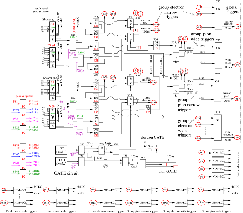
Figure 2: [Color online] Electronics diagram for the Right HRS DAQ used by the PVDIS experiment. The Sum8’s, discriminators and logic modules for two groups are shown, as well as the location of tagger signal inputs, setup of the GATE circuit using scintillator (SC) and gas Cherenkov (GC) signals, the logic units for combining triggers from all eight groups into final triggers, the counting scalers, and the monitoring fastbus TDCs. The discriminators had three different levels of threshold settings: low threshold (DL) was used on the total shower (TS) signals to form pion triggers; medium (DM) and high thresholds (DH) were used on preshower (PS) and TS signals respectively to form electron triggers. During the experiment the thresholds were approximately -20 mV for DL and DM, and in the range $(-50,-70)$ mV for DH depending on the momentum setting of the spectrometer. Electronics for the Left HRS are similar except for the grouping scheme.

A schematic diagram of the DAQ electronics for the Right HRS is shown in Fig. 2. Preliminary electron and pion triggers were formed by passing shower (SS) and preshower (PS) signals and their sums, called total shower (TS) signals, through discriminators with different thresholds. For electron triggers, logical ANDs of the PS discriminator and the TS discriminator outputs were used. For pions, low threshold discriminators on the TS signal alone were sent to logical OR modules to produce preliminary triggers. Additional background rejection was provided by the “GATE” circuit, which combined signals from the gas Cherenkov (GC) and the “T1” signal [6] from the scintillators (SC). Each valid coincidence between GC and T1 would produce a 150-ns wide electron GATE signal that allowed an output to be formed by the logical AND modules from the preliminary electron triggers. Each valid T1 signal without the GC signal would produce a 150-ns wide pion GATE signal that allowed an output to be formed by the logical OR modules from the preliminary pion triggers. The outputs of the logical AND and OR modules are called group electron and pion triggers, respectively. All six (eight) group electron or pion triggers were then ORed together to form the global electron or pion trigger for the Left (Right) HRS. All group and the final electron and pion triggers were counted using scalers. Because pions do not produce large enough lead-glass signals to trigger the high threshold TS discriminators for the electron triggers, pions do not introduce extra counting deadtime for the electron triggers. However, the 150-ns width of the electron GATE signal would cause pion contamination in the electron trigger. This effect will be presented in Section 4.

In order to monitor the counting deadtime of the DAQ, two identical paths of electronics were constructed. The only difference between the two paths is in the PS and the TS discriminator output widths, set at 30 ns and 100 ns for the “narrow” and the “wide” paths, respectively. The scalers are rated for 250 MHz (4 ns deadtime) and therefore do not add to the deadtime. In addition, the output width of all logic modules was set to 15 ns, so the deadtime of the DAQ for each group is dominated by the deadtime of the discriminators. Detailed analysis of the DAQ deadtime will be presented in Section 5.

The SUM8 modules used for summing all lead-glass signals also served as fan-out modules, providing exact copies of the input PMT signals. These copies were sent to the standard HRS DAQ for calibration. During the experiment, data were collected at low rates using reduced beam currents with both DAQs functioning, such that a direct comparison of the two DAQs could be made. Vertical drift chambers were used during these low rate DAQ studies. Outputs from all discriminators, signals from the scintillator and the gas Cherenkov, and all electron and pion group and global triggers were sent to Fastbus TDCs (fbTDC) and were recorded in the standard DAQ. Data from these fbTDCs were used to align the amplitude spectrum and timing of all signals. They also allowed the study of the Cherenkov and the lead-glass detector performance for the new DAQ.

Full sampling of partial analog signals was done using Flash-ADCs (FADCs) at low rates intermittently during the experiment. For one group on the Left and one group on the Right HRS, the preshower and the shower SUM8 outputs, the intermediate logical signals of the DAQ, and the output electron and pion triggers were recorded. These FADC data provided a study of pileup effects to confirm the deadtime simulation and to provide the input parameters for the simulation, specifically the rise and fall times of the signals and their widths.

3 Overview of Kinematics

During the experiment data were taken at two deep inelastic scattering (DIS) kinematics at $Q^{2}=1.1$ and $1.9$ (GeV/$c$)². These were the main production kinematics and will be referred to as DIS#1 and DIS#2, respectively. Due to limitation of the spectrometer magnets, DIS#1 was taken only on the Left HRS, while DIS#2 was taken on both Left and Right HRSs. In addition, data were taken at five kinematics within or near the nucleon resonance region with their invariant mass $W$ between the $\Delta(1232)$ resonance and just above $W=2$ GeV. These data were used for the purpose of radiative corrections and will be referred to as RES I through V (although kinematics V was located slightly above $W=2$ GeV). Data for each of the resonance settings were taken only with one HRS because of the spectrometer magnet limitations as well as to optimize the beam time allocation. The kinematic settings are shown in Table 1 along with the observed electron rate $R_{e}$ and the pion to electron ratio $R_{\pi^{-}}/R_{e}$ in the HRS. The highest electron rate occurred at RES II at approximately 600 kHz.

Kine#	HRS	$E_{b}$ (GeV)	$\theta_{0}$	$E^{\prime}_{0}$ (GeV)	$R_{e}$(kHz)	$R_{\pi^{-}}/R_{e}$
DIS#1	Left	6.067	$12.9^{\circ}$	$3.66$	$\approx 210$	$\approx 0.5$
DIS#2	Left & Right	6.067	$20.0^{\circ}$	$2.63$	$\approx 18$	$\approx 3.3$
RES I	Left	4.867	$12.9^{\circ}$	$4.0$	$\approx 300$	$<\approx 0.25$
RES II	Left	4.867	$12.9^{\circ}$	$3.55$	$\approx 600$	$<\approx 0.25$
RES III	Right	4.867	$12.9^{\circ}$	$3.1$	$\approx 400$	$<\approx 0.4$
RES IV	Left	6.067	$15^{\circ}$	$3.66$	$\approx 80$	$<\approx 0.6$
RES V	Left	6.067	$14^{\circ}$	$3.66$	$\approx 130$	$<\approx 0.7$

Table 1: Overview of kinematics settings during the experiment, including: the beam energy $E_{b}$, the spectrometer central angle setting $\theta_{0}$ and central momentum setting $E^{\prime}_{0}$, the observed electron rate $R_{e}$ and the $\pi^{-}/e$ ratio $R_{\pi^{-}}/R_{e}$.

4 DAQ PID Performance

The PID performance of the DAQ system was studied with calibration runs taken at low beam currents using fbTDC signals along with ADC data of all detector signals recorded by the standard DAQ. Events that triggered the DAQ would appear as a timing peak in the corresponding fbTDC spectrum of the standard DAQ, and a cut on this peak can be used to select those events. Figure 3 shows the preshower vs. shower signals for group 2 on the Left HRS. A comparison between no fbTDC cut and with cut on the fbTDC signal of the electron wide trigger from this group clearly shows the hardware PID cuts.

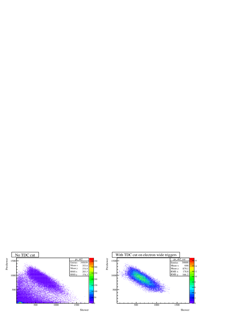
Figure 3: Preshower vs. Shower ADC data (sum of 8 blocks each) for group 2 on the Left HRS, without the fbTDC cut (left panel) and with cut on the group 2 electron wide trigger fbTDC signal (right panel). This clearly shows the thresholds of the preshower and the total shower signals, indicating that the DAQ is selecting the correct events as electrons.

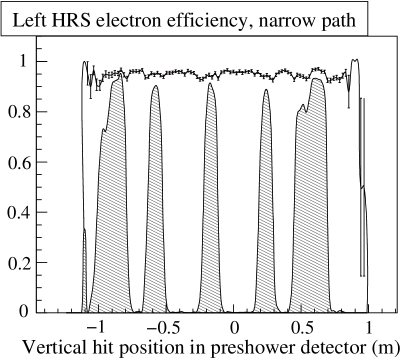
Figure 4: Electron detection efficiency (left) and pion rejection factor (right) vs. vertical (dispersive) hit position of the particle in the preshower detector for the narrow electron triggers in the Left HRS. An 8-minute run with a reduced beam current of $2$ $\mu$A at kinematics DIS #2 was used in this evaluation. For electron efficiencies, the total efficiency and the statistical error bars are shown as the curve, while the shaded area indicates events that were recorded by two adjacent groups. The average electron efficiency achieved by the lead glass detector alone for this run is $[94.60\pm 0.11$(stat.)$]\%$ and the average pion rejection factor is $[76.2\pm 1.5$(stat.)$]:1$. PID performance for the wide path and the Right HRS are similar.

Electron efficiency and pion rejection factors of the lead-glass detector on the Left HRS during a one-hour run are shown in Fig. 4 as functions of the location of the hit of the particle in the preshower detector. PID performance on the Right HRS is similar. Electron efficiency from wide groups is slightly higher than from narrow groups because there is less event loss due to timing misalignment when taking the coincidence between the preshower and the total shower discriminator outputs. Variations in the electron efficiency across the spectrometer acceptance effectively influence the $Q^{2}$ of the measurement. For this reason, low-rate calibration data were taken daily during the experiment to monitor the DAQ PID performance, and corrections were applied to the asymmetry data.

The gas Cherenkov detector signals were read out by 10 PMTs on both the Left and the Right HRS. Signals from all 10 PMTs were summed in an analog-sum module and sent to a discriminator. The discriminator output was sent to the DAQ (as shown in Fig. 2) as well as to fbTDCs. Figure 5 shows the Cherenkov ADC sum with and without the fbTDC cut, which clearly shows the capability of rejecting pions.

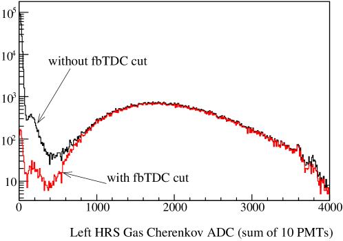
Figure 5: [Color online] Gas Cherenkov ADC data (sum of 10 PMTs) for the Left HRS during a one-hour run at kinematics DIS #2, with a fbTDC cut on the Cherenkov discriminator output and without. The beam current during this run was about 100 $\mu$A, the incident electron rate on the detector was about 23 kHz with a pion to electron rate ratio of approximately 3.5. The electron efficiency achieved by the gas Cherenkov alone for this kinematics on the Left HRS was approximately 99% with a pion rejection of approximately 300:1, see Table 2. The discriminator clearly selected electrons while rejecting pions.

As described in the Introduction, pion contamination in the electron trigger would affect the measured electron asymmetry as $A_{m}=(1-f_{\pi/e})A_{e}+f_{\pi/e}A_{\pi}$ where $A_{m}$ and $A_{e}$ are the measured and the true electron asymmetries, respectively, and $A_{\pi}$ is the parity violation asymmetry of pion production. The pion contamination in the electron trigger, $f_{\pi/e}$, comes from two effects: There is a small possibility that a pion could trigger both the lead-glass and the gas Cherenkov detectors, causing a false electron trigger output. This possibility is determined by the direct combination of the pion rejection factors of the two detectors and is below $10^{-4}$. A larger effect comes from the width of the electron GATE signal: Since each coincidence between the gas Cherenkov and the scintillator signals would open the electron counting GATE by 150 ns, while the DAQ deadtime of the lead-glass detector is less than this value, pions that arrived after the DAQ deadtime but before the closing of the electron GATE signal would cause a false electron trigger. The sum of the two effects can be written as

$$f_{\pi/e,n(w)} = \frac{R_{\pi}\eta^{GC}_{\pi}\eta^{LG}_{\pi}}{R_{e}\eta_{e}^{GC}\eta_{e}^{LG}}+\frac{R_{\pi}\eta^{LG}_{\pi}\{R_{e}\eta_{e}^{GC}[150~{}\mathrm{ns}-\tau_{n(w)}]\}}{R_{e}\eta_{e}^{GC}\eta_{e}^{LG}}$$ (3)

where $R_{e}$ and $R_{\pi}$ are the input electron and the pion rates, respectively; $\eta_{e}^{LG(GC)}$ is the electron detection efficiency of the lead-glass (gas Cherenkov) detectors, and $\eta_{\pi}^{LG(GC)}$ is the pion detection efficiency, i.e., the inverse of the rejection factor, of the lead-glass (gas Cherenkov) detector. The DAQ group deadtime of the lead-glass detector for the narrow (wide) path, $\tau_{n(w)}$, is approximately 60 ns (100-110 ns) and the analysis obtaining these results will be presented in the next section. The term $R_{e}\eta_{e}^{GC}[150~{}\mathrm{ns}-\tau_{n(w)}]$ gives the probability of a pion’s arriving within a valid electron GATE signal and thus such a pion can not be rejected by the gas Cherenkov detector.

The electron detection efficiency and pion rejection factor averaged throughout the data production period are shown in Tables 2 and 3 for DIS and resonance kinematics, respectively, along with the resulting pion contamination $f_{\pi/e}$ evaluated separately for the narrow and the wide paths.

DIS Kinematics and Spectrometer combinations
	DIS# 1	DIS# 2
HRS	Left	Left	Right
Electron detection efficiency $\eta_{e}$ ($\%$)
GC	$99.14\pm 0.02$	$99.03\pm 0.03$	$98.19\pm 0.06$
LG, n	$91.93\pm 0.04$	$94.50\pm 0.06$	$94.36\pm 0.04$
LG, w	$92.88\pm 0.04$	$95.79\pm 0.06$	$95.23\pm 0.04$
GC+LG, n	$91.14\pm 0.04$	$93.58\pm 0.06$	$92.65\pm 0.07$
GC+LG, w	$92.08\pm 0.04$	$94.86\pm 0.06$	$93.51\pm 0.07$
Pion rejection $1/\eta_{\pi}$
GC	$158.6\pm 3.5$	$301.2\pm 5.2$	$414.3\pm 6.2$
LG, n	$101.5\pm 1.6$	$78.9\pm 0.9$	$72.7\pm 0.3$
LG, w	$103.9\pm 1.7$	$81.5\pm 1.0$	$74.3\pm 0.3$
Pion contamination in the electron trigger $f_{\pi/e}$, narrow path ($\times 10^{-4}$)
$f_{\pi/e,n}$	$1.07$	$1.97$	$1.30$
(stat.)	$\pm 0.02$	$\pm 0.03$	$\pm 0.01$
(syst.)	$\pm 0.24$	$\pm 0.18$	$\pm 0.10$
(total)	$\pm 0.24$	$\pm 0.18$	$\pm 0.10$
Pion contamination in the electron trigger $f_{\pi/e}$, wide path ($\times 10^{-4}$)
$f_{\pi/e,w}$	$0.72$	$1.64$	$0.92$
(stat.)	$\pm 0.01$	$\pm 0.03$	$\pm 0.01$
(syst.)	$\pm 0.22$	$\pm 0.17$	$\pm 0.13$
(total)	$\pm 0.22$	$\pm 0.17$	$\pm 0.13$

Table 2: Average electron detection efficiency and pion rejection factor of electron triggers achieved for the DIS kinematics through the lead glass (LG) and the gas Cherenkov (GC) detectors, respectively, and the combined performance. The error bars of the efficiencies and the rejection factors are statistical only. The error bars for $f_{\pi/e}$, $\Delta f_{\pi/e,n(w)}$, are shown separately for statistical uncertainties, systematic uncertainties due to our understanding of the rates, detector efficiencies and deadtimes, and day-to-day variations in the measured detector efficiencies.

Resonance Kinematics and Spectrometer combinations
	RES I	RES II	RES III	RES IV	RES V
HRS	Left	Left	Right	Left	Left
Electron detection efficiency $\eta_{e}$ ($\%$)
GC	$99.16\pm 0.09$	$99.17\pm 0.13$	$98.59\pm 0.11$	$99.41\pm 0.07$	$99.16\pm 0.11$
LG, n	$97.73\pm 0.07$	$97.13\pm 0.07$	$98.14\pm 0.06$	$84.71\pm 0.18$	$84.66\pm 0.21$
LG, w	$98.32\pm 0.07$	$97.83\pm 0.08$	$98.56\pm 0.06$	$85.31\pm 0.18$	$85.88\pm 0.23$
GC+LG, n	$96.91\pm 0.11$	$96.32\pm 0.15$	$96.76\pm 0.12$	$84.20\pm 0.20$	$83.95\pm 0.24$
GC+LG, w	$97.49\pm 0.11$	$97.02\pm 0.15$	$97.17\pm 0.13$	$84.80\pm 0.20$	$85.16\pm 0.26$
Pion rejection $1/\eta_{\pi}$
GC	$82.8\pm 9.2$	$97.7\pm 10.5$	$195.0\pm 24.5$	$149.6\pm 10.2$	$151.4\pm 11.5$
LG, n	$43.6\pm 4.0$	$57.4\pm 5.4$	$37.0\pm 0.9$	$182.4\pm 15.1$	$207.2\pm 20.5$
LG, w	$39.4\pm 3.6$	$53.5\pm 5.1$	$33.9\pm 0.9$	$171.4\pm 14.1$	$201.1\pm 23.5$
Pion contamination in the electron trigger $f_{\pi/e}$, narrow path ($\times 10^{-4}$)
$f_{\pi/e,n}$	$0.79$	$2.40$	$3.82$	$0.26$	$0.45$
(stat.)	$\pm 0.02$	$\pm 0.06$	$\pm 0.02$	$\pm 0.01$	$\pm 0.01$
(syst.)	$\pm 0.11$	$\pm 0.19$	$\pm 0.23$	$\pm 0.02$	$\pm 0.03$
(total)	$\pm 0.11$	$\pm 0.20$	$\pm 0.23$	$\pm 0.03$	$\pm 0.03$
Pion contamination in the electron trigger $f_{\pi/e}$, wide path ($\times 10^{-4}$)
$f_{\pi/e,w}$	$0.54$	$1.50$	$2.14$	$0.22$	$0.32$
(stat.)	$\pm 0.02$	$\pm 0.04$	$\pm 0.02$	$\pm 0.01$	$\pm 0.01$
(syst.)	$\pm 0.14$	$\pm 0.25$	$\pm 0.48$	$\pm 0.03$	$\pm 0.04$
(total)	$\pm 0.15$	$\pm 0.25$	$\pm 0.48$	$\pm 0.03$	$\pm 0.04$

Table 3: Average electron detection efficiency and pion rejection factor of electron triggers achieved for the resonance kinematics through the lead glass (LG) and the gas Cherenkov (GC) detectors, respectively, and the combined performance. The error bars of the efficiencies and the rejection factors are statistical only. The error bars for $f_{\pi/e}$, $\Delta f_{\pi/e,n(w)}$, are shown separately for statistical uncertainties, systematic uncertainties due to our understanding of the rates, detector efficiencies and deadtimes, and day-to-day variations in the measured detector efficiencies.

As shown in Tables 2-3, the overall pion contamination was on the order of $2\times 10^{-4}$ or lower throughout the experiment. Because pions are produced from nucleon resonance decays, the parity violation asymmetry of pion production is expected to be no larger than that of scattered electrons with the same momentum. This was confirmed by asymmetries formed from pion triggers during this experiment. The uncertainty in the electron asymmetry due to pion contamination is therefore on the order of $2\times 10^{-4}$ and is negligible compared with the $3-4\%$ statistical uncertainty.

To understand fully the effect of pion background on the measured electron asymmetry, it is important to extract asymmetries of the pion background to confirm that they are indeed smaller than the electron asymmetry. A complete PID analysis was carried out on the pion triggers of the DAQ where the electron contamination in the pion trigger $f_{e/\pi}$ was evaluated in a similar method as $f_{\pi/e}$ above, following

$$f_{e/\pi,n(w)}=\frac{R_{e}\xi^{GC}_{e}\xi^{LG}_{e}}{R_{\pi}\xi_{\pi}^{GC}\xi_{\pi}^{LG}}+\frac{R_{e}\xi^{LG}_{e}\{R_{\pi}\xi_{\pi}^{GC}[150~{}\mathrm{ns}-\tau_{n(w)}]\}}{R_{\pi}\xi_{\pi}^{GC}\xi_{\pi}^{LG}}$$ (4)

where as before $R_{e}$ and $R_{\pi}$ are the electron and the pion rates incident on the detectors, respectively; the detection efficiencies $\xi$ are now defined for the pion triggers of the DAQ: $\xi_{e}^{LG(GC)}$ is the electron detection efficiency of the lead-glass (gas Cherenkov) detectors, and $\xi_{\pi}^{LG(GC)}$ is the pion detection efficiency of the lead-glass (gas Cherenkov) detector. Although the goal of the pion triggers is to collect pions, only the gas Cherenkov played a role in rejecting electrons in the pion trigger, and all electrons would form valid pion triggers in the lead-glass counters. Therefore $\xi_{e}^{LG}\approx 1$ and the electron contamination is high. Results for electron contamination in the pion trigger are summarized in Tables 4 and 5.

Kinematics and Spectrometer Combinations
	DIS#1	DIS#2
HRS	Left	Left	Right
Pion detection efficiency $\xi_{\pi}$ ($\%$)
GC	$99.52\pm 0.01$	$99.73\pm 0.01$	$99.74\pm 0.01$
LG, n	$21.67\pm 0.01$	$79.72\pm 0.02$	$15.61\pm 0.01$
LG, w	$21.67\pm 0.01$	$79.71\pm 0.02$	$15.60\pm 0.01$
GC+LG, n	$21.57\pm 0.01$	$79.70\pm 0.02$	$15.57\pm 0.01$
GC+LG, w	$21.57\pm 0.01$	$79.69\pm 0.02$	$15.56\pm 0.01$
Electron rejection $1/\xi_{e}$
GC	$31.42\pm 0.78$	$89.44\pm 2.48$	$48.48\pm 1.55$
LG, n	$1.0468\pm 0.0003$	$1.0487\pm 0.0005$	$1.0271\pm 0.0002$
LG, w	$1.0469\pm 0.0003$	$1.0499\pm 0.0005$	$1.0279\pm 0.0002$
Electron contamination in pion triggers $f_{e/\pi}$, narrow path
$f_{e/\pi,n}$	$0.2653$	$0.0331$	$0.0103$
(stat.)	$\pm 0.0029$	$\pm 0.0006$	$\pm 0.0002$
(syst.)	$\pm 0.0602$	$\pm 0.0033$	$\pm 0.0013$
(total)	$\pm 0.0603$	$\pm 0.0034$	$\pm 0.0013$
Electron contamination in pion triggers $f_{e/\pi}$, wide path
$f_{e/\pi,w}$	$0.2176$	$0.0281$	$0.0091$
(stat.)	$\pm 0.0029$	$\pm 0.0006$	$\pm 0.0002$
(syst.)	$\pm 0.0573$	$\pm 0.0036$	$\pm 0.0012$
(total)	$\pm 0.0573$	$\pm 0.0037$	$\pm 0.0013$

Table 4: Average pion detection efficiency and electron rejection factor of pion triggers achieved for DIS kinematics through the lead glass (LG) and the gas Cherenkov (GC) detectors, respectively, and the combined performance. The error bars of the efficiencies and the rejection factors are statistical only. The error bars for $f_{e/\pi}$, $\Delta f_{e/\pi,n(w)}$, are shown separately for statistical uncertainties, systematic uncertainties, and day-to-day variations in the measured detector efficiencies.

Kinematics and Spectrometer Combinations
	RES I	RES II	RES III	RES IV	RES V
HRS	Left	Left	Right	Left	Left
Pion detection efficiency $\xi_{\pi}$ ($\%$)
GC	$98.82\pm 0.13$	$98.96\pm 0.11$	$99.43\pm 0.07$	$99.38\pm 0.04$	$99.47\pm 0.04$
LG, n	$26.27\pm 0.62$	$25.65\pm 0.55$	$82.78\pm 0.16$	$21.16\pm 0.25$	$20.69\pm 0.28$
LG, w	$27.07\pm 0.65$	$26.14\pm 0.57$	$83.60\pm 0.17$	$22.54\pm 0.26$	$20.71\pm 0.28$
GC+LG, n	$25.96\pm 0.64$	$25.39\pm 0.56$	$82.31\pm 0.17$	$21.03\pm 0.25$	$20.58\pm 0.28$
GC+LG, w	$26.75\pm 0.66$	$25.87\pm 0.58$	$83.12\pm 0.18$	$22.40\pm 0.26$	$20.60\pm 0.28$
Electron rejection $1/\xi_{e}$
GC	$121.36$	$118.33$	$72.91$	$101.43$	$74.80$
	$\pm 21.71$	$\pm 34.02$	$\pm 5.67$	$\pm 16.59$	$\pm 13.57$
LG, n	$1.0167$	$1.0194$	$1.0114$	$1.0677$	$1.0652$
	$\pm 0.0006$	$\pm 0.0006$	$\pm 0.0005$	$\pm 0.0014$	$\pm 0.0016$
LG, w	$1.0167$	$1.0105$	$1.0064$	$1.0344$	$1.0541$
	$\pm 0.0006$	$\pm 0.0006$	$\pm 0.0005$	$\pm 0.0013$	$\pm 0.0016$
Electron contamination in pion triggers $f_{e/\pi}$, narrow path
$f_{e/\pi,n}$	$0.4114$	$0.3155$	$0.0849$	$0.1852$	$0.1871$
(stat.)	$\pm 0.0117$	$\pm 0.0061$	$\pm 0.0006$	$\pm 0.0062$	$\pm 0.0058$
(syst.)	$\pm 0.0163$	$\pm 0.0151$	$\pm 0.0029$	$\pm 0.0038$	$\pm 0.0050$
(total)	$\pm 0.0201$	$\pm 0.0163$	$\pm 0.0030$	$\pm 0.0073$	$\pm 0.0077$
Electron contamination in pion triggers $f_{e/\pi}$, wide path
$f_{e/\pi,w}$	$0.3423$	$0.2409$	$0.0633$	$0.1661$	$0.1598$
(stat.)	$\pm 0.0116$	$\pm 0.0062$	$\pm 0.0006$	$\pm 0.0063$	$\pm 0.0057$
(syst.)	$\pm 0.0200$	$\pm 0.0190$	$\pm 0.0059$	$\pm 0.0049$	$\pm 0.0064$
(total)	$\pm 0.0231$	$\pm 0.0200$	$\pm 0.0060$	$\pm 0.0080$	$\pm 0.0086$

Table 5: Average pion detection efficiency and electron rejection factor of pion triggers achieved for resonance kinematics through the lead glass (LG) and the gas Cherenkov (GC) detectors, respectively, and the combined performance. The error bars of the efficiencies and the rejection factors are statistical only. The error bars for $f_{e/\pi}$, $\Delta f_{e/\pi,n(w)}$, are shown separately for statistical uncertainties, systematic uncertainties, and day-to-day variations in the measured detector efficiencies.

5 DAQ Deadtime

Deadtime is the amount of time after an event during which the system is unable to record another event. Identifying the exact value of the deadtime is always a challenge in counting experiments. By having a narrow and a wide path, we can observe the trend in the deadtime: The wider path should have higher deadtime. By matching the observed trend with our simulation we can benchmark and confirm the result of our deadtime simulation. In addition, dividing lead-glass blocks into groups greatly reduces the deadtime loss in each group compared with summing all blocks together and forming only one final trigger.

To illustrate the importance of the deadtime, consider its effect on the asymmetry $A$. For a simple system with only one contribution to the deadtime loss $\delta$, the observed asymmetry $A_{O}$ is related to the true asymmetry $A$ according to $A_{O}=(1-\delta)A$.  In this experiment $\delta$ was expected to be on the order of (1-2)%. Since the statistical accuracy of the asymmetry is (3-4)%, it was desirable to know $\delta$ with a (10-20)% relative accuracy so that it would become a negligible systematic error. The DAQ used in this experiment, however, was more complex and had three contributions to the deadtime as listed below:

1. The “group” deadtime: deadtime due to discriminators and logical AND modules used to form group triggers.

2. The “GATE” deadtime: deadtime from the GATE circuit that used scintillators and gas Cherenkov signals to form the GATE signals, which controlled the AND (OR) module of each group to form group electron (pion) triggers.

3. The “OR” deadtime: deadtime due to the logical OR module used to combine all group triggers into final global triggers.

The total deadtime is a combination of all three. In order to evaluate the DAQ deadtime, a full-scale trigger simulation is necessary. This trigger simulation will be described in the next section followed by results on the group, GATE, and OR deadtime as well as on the total deadtime correction that was applied to the asymmetry data.

5.1 Trigger Simulation

The Hall A Trigger Simulation (HATS) was developed for the purpose of deadtime study for this experiment. The inputs to HATS include the analog signals for preshower, shower, scintillator and gas Cherenkov. The signal amplitudes were provided by ADC data from low-current runs, and the signal rates were from high-current production runs. The rise and fall times for the preshower and shower SUM8 outputs play an important role in HATS. The signal shape is simulated by the function $S(t)=Ate^{-t/\tau}$, where $A$ is related to the amplitude of the signal, and the time constant $\tau$ was determined from FADC data, see Fig. 6.

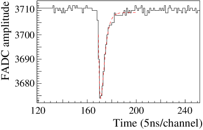
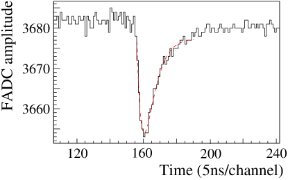
Figure 6: [Color online] Calibration of time constants $\tau$ for Preshower (left) and Shower (right) of the Right HRS. The FADC snapshots (histograms) is compared with the fit $S(t)=Ate^{-t/\tau}$ (smooth dashed curves). The time constant $\tau$ was found to be approximately $11$ ns for the Right HRS Preshower, and $21-22$ ns for the Left HRS Preshower and Shower as well as for the Right HRS Shower.

With the recorded DAQ electronics and delay cables, HATS first rebuilds the DAQ system on the software level. At each nano-second, detector input signals are generated randomly according to the actual event rates and signal shape, and HATS simulates output signals from all discriminators, AND, and OR modules. Figure  7 shows a fraction of the DAQ electronics and the simulated results for a very short time period. By comparing output with input signals, HATS provides results on the fractional loss due to deadtime for all group and global triggers with respect to the input signal.

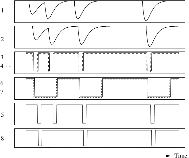
Figure 7: Top: A fraction of the group electron trigger. Each point corresponds to: 1 – Shower sum of the group; 2 – Total shower sum of the group; 3 – Total shower discriminator output (high threshold), narrow path; 4 – Preshower discriminator output (medium threshold), narrow path; 5 – group electron trigger, narrow path; 6 – Total shower discriminator output, wide path; 7 – Preshower discriminator output, wide path; 8 – group electron trigger, wide path. Bottom: Signals 1-8 as simulated by HATS. One can see that the second physical event is recorded by the narrow path group trigger (5) but not the wide path (8) due to deadtime loss.

5.2 Group Deadtime Measurement

In order to study the group deadtime, a high rate pulser signal (“tagger”) was mixed with the Cherenkov and all preshower and total shower signals using analog summing modules, see Figs. 2 and 8. In the absence of all detector signals, a tagger pulse produces without loss an electron trigger output and a “tagger-trigger coincidence” pulse between this output and the “delayed tagger” – the tagger itself with an appropriate delay to account for the DAQ response time. When high-rate detector signals are present, however, some of the tagger pulses would not be able to trigger the DAQ due to deadtime. The deadtime loss in the electron trigger output with respect to the tagger input has two components:

1. The count loss $R_{o}/R_{i}$: When a detector PMT signal precedes the tagger signal by a time interval $\delta t$ shorter than the DAQ deadtime but longer than $w+t_{1}$, the tagger signal is lost and no coincidence output is formed. Here $w$ is the width of the electron trigger output and $t_{1}$ is the time interval by which the delayed tagger precedes the tagger’s own trigger output, see Fig. 8. During the experiment $w$ was set to 15 ns for all groups, and $t_{1}$ was measured at the end of the experiment and found to be between 20 and 40 ns for all narrow and wide groups of the two HRSs.

2. The pileup fraction $p$: When a PMT signal precedes the tagger signal by a time interval $\delta t$ shorter than $w+t_{1}$, there would be a coincidence output between the delayed tagger and the electron output triggered by the detector PMT signal. If furthermore $\delta t$ is less than the DAQ deadtime (which is possible for this experiment since the deadtime is expected to be as long as 100 ns for the wide path), the tagger itself is lost due to deadtime, and the tagger-trigger coincidence is a false count and should be subtracted. In the case where $\delta t$ is shorter than $w+t_{1}$ but longer than the DAQ deadtime (not possible for this experiment but could happen in general), the tagger itself also triggers a tagger-trigger coincidence, but in this case, there are two tagger-trigger coincidence events. Both are recorded by the fbTDC if working in the multi-hit mode, and one is a false count and should be subtracted.

   The pileup effect can be measured using the delay between the tagger-trigger coincidence output and the input tagger. This is illustrated in Fig. 8 and the pileup effect contributes to both $I_{1}$ and $I_{2}$ regions of the fbTDC spectrum. The $I_{1}$ distribution is produced by PMT pulses that arrive after the delayed tagger signal but before the tagger signal would propagate through the trigger electronics. Peak $I_{2}$ occurs when a PMT pulse arrives at the coincidence module earlier than the delayed tagger signal but which forms a coincidence with the delayed tagger signal, giving an output whose time is set by the latter. Fractions of $I_{1}$ and $I_{2}$ relative to $I_{0}$ are expected to be $I_{1}/I_{0}=Rt_{1}$ and $I_{2}/I_{0}=Rw$, respectively, where $R$ is the PMT signal rate. The pileup effect was measured using fbTDC spectrum for electron narrow and wide triggers for all groups. Data for $I_{1,2}$ extracted from fbTDC agree very well with the expected values.

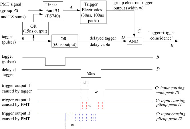
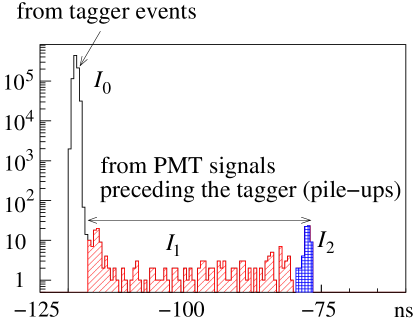
Figure 8: [Color online] Top: schematic diagram for the tagger setup and signal timing sequence. The two logical OR units immediately following the tagger input “B” serve as width adjusters. Bottom: fbTDC spectrum for the relative timing between tagger-trigger coincidence and the input tagger. The fbTDC module worked in a common stop and the multi-hit mode. Two different scenarios are shown: 1) Main peak $I_{0}$ (hollow peak): when there is no PMT signal preceding the tagger, the tagger triggers the DAQ and forms a tagger-trigger coincidence. 2) Pileup events $I_{1}$ (light-shaded region) and $I_{2}$ (heavy-shaded region): when there is a PMT signal preceding the tagger by a time interval shorter than $w+t_{1}$, the PMT signal triggers the DAQ and forms a tagger-trigger coincidence signal with the delayed tagger.

The relative loss of tagger events due to DAQ deadtime is evaluated as

$${D=1-(1-p)(R_{o}/R_{i}),}$$ (5)

where $R_{i}$ is the input tagger rate, $R_{o}$ is the output tagger-trigger coincidence rate, and $p=(I_{1}+I_{2})/I_{0}$ is a correction factor for pileup effects as defined in Fig. 8. Results for the deadtime loss $D$ are shown in Figs. 9 and 10, for group 4 on the left HRS and group 4 on the right HRS, respectively, and are compared with simulation. Different beam currents between 20 and 100 $\mu$A were used in this dedicated deadtime measurement. In order to reduce the statistical fluctuation caused by the limited number of trials in the simulation within a realistic computing time, simulations were done at higher rates than the actual measurement.

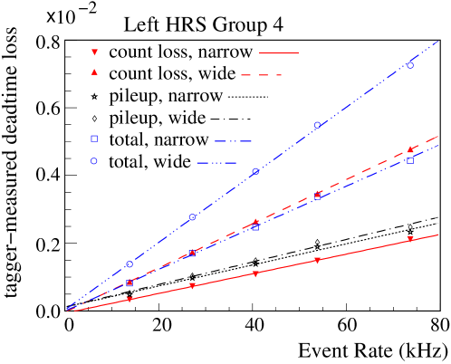
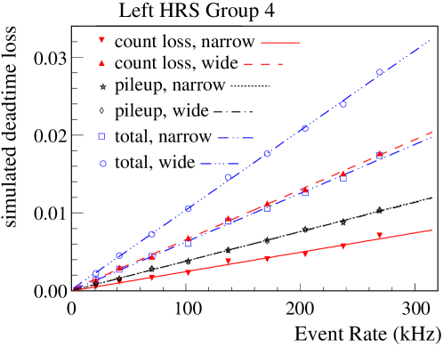
Figure 9: [Color online] Deadtime loss vs. event rate from the tagger method for group 4 on the Left HRS. Top: actual deadtime loss from tagger measurements; Bottom: simulated deadtime loss of the tagger. The tagger fractional count loss $1-R_{o}/R_{i}$ (fit by solid and dashed lines) and the pileup correction $p$ (fit by dotted and dash-dotted lines) are combined to form the total group deadtime $D$ (fit by dash-double-dotted and dash-triple-dotted lines). These data were taken (or simulated) at kinematics DIS #1. To minimize the statistical uncertainty while keeping the computing time reasonable, the simulation used higher event rates than the tagger measurement. The total group deadtime can be determined from the linear fit slope coefficients: tagger data narrow $(61.5\pm 0.2)\times 10^{-9}$ s, wide $(99.9\pm 0.3)\times 10^{-9}$ s, simulation narrow $(62.5\pm 1.4)\times 10^{-9}$ s, wide $(102\pm 1.3)\times 10^{-9}$ s. Group 4 is from the central blocks of the lead-glass detector and has the highest rate among all groups.

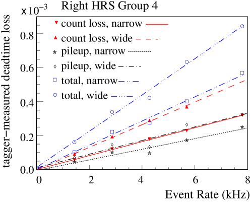
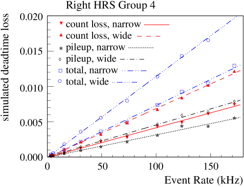
Figure 10: [Color online] Deadtime loss vs. group event rate from the tagger method for group 4 on the Right HRS. Top: tagger data; Bottom: simulation. These data were taken (or simulated) at kinematics DIS #2. The total group deadtime can be determined from the linear fit slope coefficients: tagger data narrow $(71.1\pm 0.9)\times 10^{-9}$ s, wide $(107\pm 1.2)\times 10^{-9}$ s, simulation narrow $(73.9\pm 1.5)\times 10^{-9}$ s, wide $(115\pm 1.5)\times 10^{-9}$ s. Group 4 is from the central blocks of the lead-glass detector and has the highest rate among all groups. See Fig. 9 caption for more details.

The slope of the tagger loss vs. event rate, as shown in Figs. 9 and 10, gives the value of group deadtime in seconds. One can see that the deadtime for the wide path is approximately 100 ns as expected. The deadtime for the narrow path, on the other hand, is dominated by the input PMT signal width (typically 60-80 ns) instead of the 30-ns discriminator width. The simulated group deadtime agrees with the data at a 10% level or better, for both HRSs and for both wide and narrow paths.

The above tagger measurements were performed at kinematics DIS#1 on the Left and DIS#2 on the Right HRS. No tagger data was available for resonance kinematics. However since the group deadtime is expected to rely only on the signal width and the module width settings, as demonstrated by the tagger data, a 10% systematic uncertainty was used for group deadtime for all kinematics.

5.3 Gate Deadtime Evaluation

Figure 11 shows the GATE electronics for both spectrometers, with the bottom panel reproducing the GATE portion of Fig. 2.

Figure 11: A zoom-in view of the GATE electronics for Left (top) and Right (bottom) spectrometers.

It contributes to the total deadtime as follows: When both the gas Cherenkov and the Scintillator are triggered by electrons, the two signals align in time and produce an electron GATE signal. However the Scintillator can be triggered by pions and other backgrounds, most of which do not trigger the Cherenkov. If an electron event arrives shortly after such background events, it triggers the Cherenkov but may not trigger the PS755 module that first processes the Scintillator signal because of the non-updating feature of PS755. In this case, the Cherenkov signal triggered by the electron may miss the Scintillator signal from the previous pion or background event and will not produce a valid electron GATE signal. Likewise, if a background event triggers the Cherenkov but not the Scintillator, it would also cause a loss to the electron events that follow shortly after. The fractional loss due to GATE deadtime can be estimated as

$$DT_{\mathrm{gate}} = R_{SC\&\overline{GC}}(w_{SC,in}-w_{SC,out})+R_{GC\&\overline{SC}}(w_{GC,in}-w_{GC,out}),$$ (6)

where $R_{SC\&\overline{GC}}(R_{GC\&\overline{SC}})$ refers to the rate of events that triggered the Scintillator (Cherenkov) but not the Cherenkov (Scintillator), $w_{SC,in(out)}$ and $w_{GC,in(out)}$ refer to the input (output) signal widths of the PS755 module that first processes the Scintillator and the Cherenkov signals in the GATE electronics, respectively. Note that if the electronics used to generate the Scintillator and the Cherenkov signals have intrinsic deadtimes themselves that are longer than $w_{SC,in}$ and $w_{GC,in}$, these intrinsic deadtimes should be used in place of the measured $w_{SC,in}$ and $w_{GC,in}$. In Eq. (6), each term on the right hand side is present only if $w_{in}>w_{out}$. From Fig. 11, the signal widths were measured to be: $w_{SC,in,\mathrm{left}}=w_{SC,in,\mathrm{Right}}=100$ ns, $w_{SC,out,\mathrm{left}}=w_{SC,out,\mathrm{Right}}=32$ ns, $w_{GC,in,\mathrm{left}}=60$ ns, $w_{GC,in,\mathrm{Right}}=100$ ns, $w_{GC,out,\mathrm{left}}=w_{GC,out,\mathrm{Right}}=70$ ns. However it was observed from the data that the Left HRS Cherenkov signal had an intrinsic deadtime of longer than 70 ns. In fact, data showed both HRSs had contributions from the two terms on the right hand side of Eq. (6).

Because trigger rates from Scintillator and the gas Cherenkov were much higher than individual group rates, the GATE deadtime could dominate the total deadtime of the DAQ, and the difference in total deadtime loss between narrow and wide paths could be smaller than that in their group deadtimes.

The GATE deadtime can be extracted from the trigger simulation HATS using the known signal widths and module settings, and be compared with the estimation of Eq. (6). In addition, evidence of the GATE deadtime can be extracted from FADC data. Figure 12 shows spectra of the timing difference between the gas Cherenkov (GC) and the Scintillator (SC) signals extracted from FADC data. Timing of the GC signal should represent the timing of an electron event, while the SC signal can be triggered by the same electron (as represented by the main peak near 0 ns), or a pion event that preceded the electron (as represented by the region $<0$ ns). The region beyond $\pm 100$ ns were pure random events since the SC signal input to the GATE electronics was only 100 ns wide. As one can see, the region between -100 and $\approx-30$ ns represents a “dead zone” where the preceding pion triggered the PS755 unit that first processed the SC signal, and caused the electron events that followed to not trigger the GATE circuit. The probability for the electron events to not be recorded by the DAQ due to this GATE deadtime is thus the ratio of the dead zone area ($N_{1}$) and the area of the main peak near 0 ns ($N_{0}$), see Fig. 12.

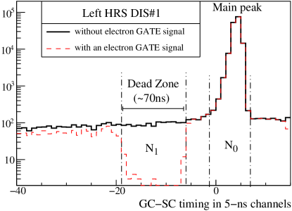
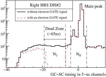
Figure 12: [Color online] Timing difference between Gas Cherenkov and Scintillator signals in 5-ns channels. These data were taken with a beam current of 110 $\mu$A and at kinematics DIS#1 on the Left and DIS#2 on the Right HRS, respectively. The fractional loss of electron events due to GATE deadtime can be estimated using the ratio of $N_{1}/N_{0}$, where $N_{1}$ is the count difference between the two spectra in the dead zone, and $N_{0}$ is the counts under the main peak near 0 ns. See text for details.

Figure 13 shows comparisons of the fractional losses due to GATE deadtime estimated using trigger simulation, the analytic method Eq. (6), and FADC data extracted from Fig. 12. The agreement between simulation and FADC was found to be better than 10% and this was used as the systematic uncertainty of the GATE deadtime. For resonance kinematics no FADC data was available. GATE deadtime for resonance data was obtained from trigger simulation and the same systematic uncertainty was used because the mechanism of the GATE deadtime was expected to remain the same throughout the experiment.

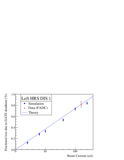
Figure 13: [Color online] Fractional loss due to GATE deadtime as a function of beam current obtained from trigger simulation (solid circles), the analytic method Eq. (6) (dashed line), and FADC data (open triangle). Error bars for simulations are statistical.

5.4 OR Deadtime Evaluation

There is no direct measurement of the logical OR deadtime, but the effect of the logical OR module is straightforward and can be calculated analytically: When two electron triggers from different groups overlap in time as they arrive at the logical OR module, they generate only one output in the global trigger. This OR deadtime loss can be calculated using the recorded trigger rates and the known trigger signal widths. To confirm the analytic method results, the OR deadtime was evaluated from trigger simulation by subtracting the group and the GATE deadtimes from the total deadtime, all three of which were direct results from the simulation. The difference between the analytic method and trigger simulation was used as the systematic uncertainty of the OR deadtime.

5.5 Total Deadtime Evaluation

The simulated deadtime loss of the global electron triggers and its decomposition into group, GATE, and OR are shown in Table 6, along with the total deadtime correction at a beam current of 100 $\mu$A. The total deadtime loss not only increases with higher electron rate $R_{e}$, but also with higher pion to electron ratio $R_{\pi}/R_{e}$ (see Table 1) which would cause larger GATE deadtime. The deadtime loss is also shown in Fig. 14 as a function of the total event rate.

Table 6: Simulated DAQ deadtime loss in percent for all kinematics and for both narrow (n) and wide (w) paths, along with the fractional contributions from group, GATE, and OR deadtimes. The fractional deadtime from OR was calculated as one minus those from group and GATE, and its uncertainty was estimated from the difference between simulation and the analytical results. The variation of group deadtime contribution among kinematics is due to changes in the rate distribution among different groups. The uncertainty of the total deadtime is the uncertainties from group, GATE and OR added in quadrature.

Kine,	Path	fractional contribution			Total deadtime
HRS		Group	GATE	OR	loss at 100$\mu$A
DIS#1,	n	$(20.6\pm 2.1)\%$	$(51.3\pm 3.5)\%$	$(28.1\pm 4.7)\%$	$(1.45\pm 0.09)\%$
Left	w	$(29.5\pm 2.4)\%$	$(45.3\pm 3.1)\%$	$(25.3\pm 4.6)\%$	$(1.64\pm 0.10)\%$
DIS#2,	n	$(5.4\pm 0.8)\%$	$(81.1\pm 5.5)\%$	$(13.5\pm 7.0)\%$	$(0.50\pm 0.04)\%$
Left	w	$(8.4\pm 0.4)\%$	$(77.3\pm 5.3)\%$	$(14.3\pm 8.0)\%$	$(0.52\pm 0.05)\%$
DIS#2,	n	$(4.6\pm 0.4)\%$	$(72.9\pm 6.0)\%$	$(22.6\pm 17.4)\%$	$(0.57\pm 0.10)\%$
Right	w	$(6.9\pm 0.7)\%$	$(71.0\pm 5.8)\%$	$(22.1\pm 17.9)\%$	$(0.58\pm 0.11)\%$
RES I,	n	$(26.3\pm 3.8)\%$	$(39.3\pm 2.7)\%$	$(34.4\pm 1.8)\%$	$(1.45\pm 0.07)\%$
Left	w	$(37.2\pm 2.1)\%$	$(34.3\pm 2.3)\%$	$(28.5\pm 3.1)\%$	$(1.66\pm 0.07)\%$
RES II,	n	$(27.6\pm 4.3)\%$	$(38.8\pm 2.7)\%$	$(33.6\pm 7.5)\%$	$(2.19\pm 0.20)\%$
Left	w	$(38.3\pm 1.9)\%$	$(33.2\pm 2.3)\%$	$(28.5\pm 7.0)\%$	$(2.56\pm 0.19)\%$
RES III,	n	$(22.9\pm 1.8)\%$	$(60.0\pm 4.9)\%$	$(17.1\pm 18.48)\%$	$(1.96\pm 0.38)\%$
Right	w	$(30.8\pm 3.1)\%$	$(51.8\pm 4.3)\%$	$(17.4\pm 12.73)\%$	$(2.27\pm 0.31)\%$
RES IV,	n	$(14.5\pm 1.9)\%$	$(63.7\pm 4.4)\%$	$(21.9\pm 3.0)\%$	$(0.75\pm 0.04)\%$
Left	w	$(21.5\pm 1.0)\%$	$(58.2\pm 4.0)\%$	$(20.3\pm 2.9)\%$	$(0.82\pm 0.04)\%$
RES V,	n	$(15.5\pm 2.1)\%$	$(68.3\pm 4.7)\%$	$(16.2\pm 5.7)\%$	$(1.03\pm 0.08)\%$
Left	w	$(22.7\pm 1.1)\%$	$(61.7\pm 4.2)\%$	$(15.6\pm 3.0)\%$	$(1.14\pm 0.06)\%$

Results shown in Table 6 provide a direct correction to the measured asymmetry, and the uncertainties are small compared with other dominant systematic uncertainties such as the approximately 2% uncertainty from beam polarizations. In practice, the deadtime correction was applied to data on a run-by-run basis with the deadtime of each run calculated using the actual beam current during the run and the linear fitting results from Fig. 14.

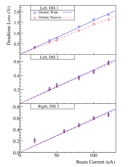
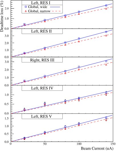
Figure 14: [Color online] Simulated deadtime loss of the global electron trigger for the three DIS spectrometer and kinematics combinations and the five resonance kinematics, for the narrow path (open triangles, fit by dashed lines) and the wide path (open squares, fit by solid lines). The error bars shown are due to statistical uncertainty of the simulation. See Table 6 for final uncertainty evaluation of the total deadtime loss.

5.6 Asymmetry Measurement

The physics asymmetries sought for in this experiment were expected to be in the order of $10^{2}$ ppm. The measured asymmetries were about $90\%$ of the expected values due to beam polarization. To understand the systematics of the asymmetry measurement, a half-wave plate (HWP) was inserted in the beamline to flip the laser helicity in the polarized source during half of the data taking period. The measured asymmetries flipped sign for each beam HWP change and the magnitude of the asymmetry remained consistent within statistical error bars.

The asymmetries can be formed from event counts of each beam helicity pair, with 33-ms of helicity right and 33-ms of helicity left beam, normalized by the beam charge. Figure 15 shows the pull distribution of these pair-wise asymmetries with the “pull” defined as

$$p_{i} \equiv (A_{i}-\langle A\rangle)/{\delta A_{i}}~{},~{}$$ (7)

where $A_{i}$ is the asymmetry extracted from the $i$-th beam helicity pair with the HWP states already corrected and $\delta A_{i}=1/\sqrt{N_{i}^{R}+N_{i}^{L}}$ its statistical uncertainty with $N_{i}^{R(L)}$ the event count from the right (left) helicity pulse of the pair, and $\langle A\rangle$ is the asymmetry averaged over all beam pairs. One can see that the asymmetry spectrum agrees to five orders of magnitude with the Gaussian distribution, as expected from purely statistical fluctuations.

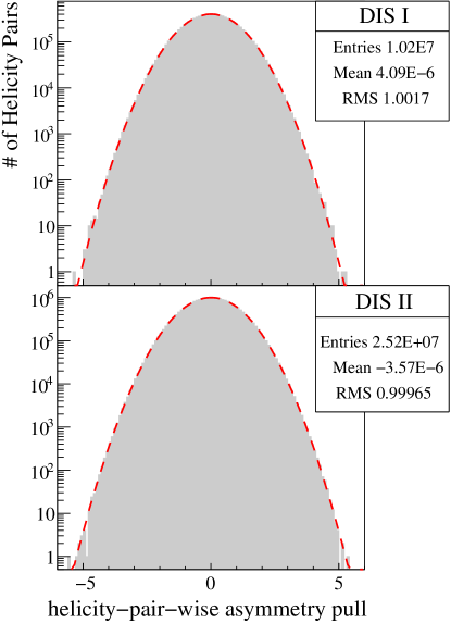
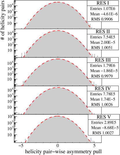
Figure 15: [Color online] Pull distribution [Eq.(7)] for the global electron narrow trigger for the three DIS spectrometer and kinematics combinations, and the five resonance kinematics. The DIS#2 distribution has both the Left and the Right HRS data combined.

6 Summary

A scaler-based counting DAQ with hardware-based particle identification was successfully implemented in the 6 GeV PVDIS experiment at Jefferson Lab to measure parity-violating asymmetries at the $10^{-4}$ level at event rates of up to 600 kHz. Asymmetries measured by the DAQ followed Gaussian distributions as expected from purely statistical measurements. Particle identification performance of the DAQ was measured and corrections were applied to the data on a day-to-day basis. The overall pion contamination in the electron sample was controlled to approximately $2\times 10^{-4}$ or lower, with an electron efficiency above 91% during most of the data production period of the experiment. The DAQ deadtime was evaluated from a full-scale timing simulation and contributed an uncertainty of no more than $0.5\%$ to the final asymmetry results. Systematic uncertainties from the pion contamination and the counting deadtime therefore were both negligible compared to the $(3-4)\%$ statistical uncertainty and other leading systematic uncertainties. Results presented here demonstrate that accurate asymmetry measurements can be performed with even higher event rates or backgrounds with this type of scaler-based DAQ.

References

- [1] JLab experiment E08-011 (previously E05-007), R. Michaels, P.E. Reimer and X.-C. Zheng, spokespersons.
- [2] R. Subedi et al., AIP proceedings of the 18th International Spin Physics Symposium (2009) 245.
- [3] Publications on the E08-011 physics asymmetries are in preparation.
- [4] R. N. Cahn and F. J. Gilman, Phys. Rev. D 17, 1313 (1978).
- [5] K. Nakamura et al. [Particle Data Group], J. Phys. G37, 075021 (2010).
- [6] J. Alcorn et al., Nucl. Instrum. Meth. A522 (2004) 294.
- [7] R. Hasty et al. [SAMPLE Collaboration], Science 290, 2117 (2000).
- [8] K. A. Aniol et al. [HAPPEX Collaboration], Phys. Rev. C 69, 065501 (2004).
- [9] A. Acha et al. [HAPPEX Collaboration], Phys. Rev. Lett. 98, 032301 (2007).
- [10] K. A. Aniol et al. [HAPPEX Collaboration], Phys. Rev. Lett. 96, 022003 (2006).
- [11] K. A. Aniol et al. [HAPPEX Collaboration], Phys. Lett. B 635, 275 (2006).
- [12] Z. Ahmed et al. [HAPPEX Collaboration], Phys. Rev. Lett. 108, 102001 (2012).
- [13] S. Abrahamyan, Z. Ahmed, H. Albataineh, K. Aniol, D. S. Armstrong, W. Armstrong, T. Averett and B. Babineau et al., Phys. Rev. Lett. 108, 112502 (2012).
- [14] C.Y. Prescott et al., Phys. Lett. B77 (1978) 347.
- [15] C.Y. Prescott et al., Phys. Lett. B84 (1979) 524.
- [16] F. E. Maas et al. [A4 Collaboration], Q**2 = 0.230-(GeV/c)**2,” Phys. Rev. Lett. 93, 022002 (2004).
- [17] F. E. Maas, K. Aulenbacher, S. Baunack, L. Capozza, J. Diefenbach, B. Glaser, T. Hammel and D. von Harrach et al., **2 = 0.108 (GeV/c)**2,” Phys. Rev. Lett. 94, 152001 (2005).
- [18] S. Baunack, K. Aulenbacher, D. Balaguer Rios, L. Capozza, J. Diefenbach, B. Glaser, D. von Harrach and Y. Imai et al., Phys. Rev. Lett. 102, 151803 (2009).
- [19] D. H. Beck, Phys. Rev. D 39, 3248 (1989).
- [20] D. S. Armstrong et al. [G0 Collaboration], Phys. Rev. Lett. 95, 092001 (2005).
- [21] D. Androic et al. [G0 Collaboration], Phys. Rev. Lett. 104, 012001 (2010).
- [22] D. Marchand, J. Arvieux, G. Batigne, L. Bimbot, A. S. Biselli, J. Bouvier, H. Breuer and R. Clark et al.Nucl. Instrum. Meth. A 586, 251 (2008).
- [23] D. Androic et al. [G0 Collaboration], Nucl. Instrum. Meth. A 646, 59 (2011).