Abstract

Three dimensional implementations of liquid state theories offer an efficient alternative to computer simulations for the atomic-level description of aqueous solutions in complex environments. In this context, we present a (classical) molecular density functional theory (MDFT) of water that is derived from first principles and is based on two classical density fields, a scalar one, the particle density, and a vectorial one, the multipolar polarization density. Its implementation requires as input the partial charge distribution of a water molecule and three measurable bulk properties, namely the structure factor and the k-dependent longitudinal and transverse dielectric constants. It has to be complemented by a solute-solvent three-body term that reinforces tetrahedral order at short range. The approach is shown to provide the correct three-dimensional microscopic solvation profile around various molecular solutes, possibly possessing H-bonding sites, at a computer cost two-three orders of magnitude lower than with explicit simulations.

Keywords: water, molecular structure, solvation, free-energy, classical density functional theory, implicit solvent method.

The numerical methods that have emerged in the second part of the last century from liquid-state theories[1, 2], including integral equation theory in the interaction-site[3, 4, 5, 6, 7, 8] or molecular[9, 10, 11, 12, 13, 14] picture, classical density functional theory (DFT)[15, 16, 17], or classical fields theory[18, 19, 20, 21], have become methods of choice for many physical chemistry or chemical engineering applications[22, 23, 24, 25]. They can yield reliable predictions for both the microscopic structure and the thermodynamic properties of molecular fluids in bulk, interfacial, or confined conditions at a much more modest computational cost than molecular-dynamics or Monte-Carlo simulations. A current challenge concerns their implementation in three dimensions in order to describe molecular liquids, solutions, and mixtures in complex environments such as atomistically-resolved solid interfaces or biomolecular media. There have been a number of recent efforts in that direction using 3D-RISM[26, 27, 28, 29, 30, 31], lattice field[32, 33] or Gaussian field[20, 34] theories. Recently, a molecular density functional theory (MDFT) approach to solvation has been introduced. [35, 36, 37, 38, 39, 40] It relies on the definition of a free-energy functional depending on the full six-dimensional position and orientation solvent density. In the so-called homogeneous reference fluid (HRF) approximation, the (unknown) excess free energy can be inferred from the angular-dependent direct correlation function of the bulk solvent, that can be predetermined from molecular simulations of the pure solvent. Compared to reference molecular dynamics calculations, such approximation was shown to be accurate for polar, non-hydrogen bonded fluids [35, 38, 39, 40, 41], but to require some corrections for water[39, 42, 43, 44].

In this paper we introduce a simplified version of MDFT that can be derived rigorously for SPC- or TIPnP-like representations of water, involving a single Lennard-Jones interaction site and distributed partial charges. In that case we will seek a simpler functional form expressed in terms of the particle density $n(\mathbf{r})$ and site-distributed polarisation density $\mathbf{P}(\mathbf{r})$, and requiring as input simpler physical quantities than the full position and orientation-dependent direct correlation function. This functional may be considered as a multipolar generalization of the generic dipolar fluid free-energy functional ${\cal F}[n(\mathbf{r}),\mathbf{P}(\mathbf{r})]$ introduced in Refs. [35, 37].

A functional of $n(\mathbf{r})$ and $\mathbf{P}(\mathbf{r})$. We start from SPC- or TIPnP-like representation of water, constituted by a single Lennard-Jones center, located on the oxygen, and $m$ charges distributed on various sites. Each molecule is supposed to be rigid with position $\mathbf{r}_{i}$ and orientation $\Omega_{i}$. For a given water configuration, we define the microscopic particle densities

$$\hat{\rho}(\mathbf{r},\Omega) = \sum^{N}_{i=1}\delta(\mathbf{r}-\mathbf{r}_{i})\delta(\Omega-\Omega_{i}),$$ (1)

$$\hat{\rho}_{n}(\mathbf{r}) = \sum^{N}_{i=1}\delta(\mathbf{r}-\mathbf{r}_{i})=\int d\Omega\hat{\rho}(\mathbf{r},\Omega),$$ (2)

and the charge and multipolar polarization density

$$\widehat{\rho}_{c}(\mathbf{r}) = \sum^{N}_{i=1}\sigma(\mathbf{r}-\mathbf{r}_{i},\Omega_{i})$$ (3)

$$= \int d\mathbf{r}^{\prime}d\Omega\,\sigma(\mathbf{r}-\mathbf{r}^{\prime},\Omega)\hat{\rho}(\mathbf{r}^{\prime},\Omega),$$

$$\widehat{\mathbf{P}}_{c}(\mathbf{r}) = \sum^{N}_{i=1}\boldsymbol{\mu}(\mathbf{r}-\mathbf{r}_{i},\Omega_{i})$$ (4)

$$= \int d\mathbf{r}^{\prime}d\Omega\,\boldsymbol{\mu}(\mathbf{r}-\mathbf{r}^{\prime},\Omega)\hat{\rho}(\mathbf{r}^{\prime},\Omega).$$

$\sigma(\mathbf{r},\Omega)$ is the molecular charge density and, according to the definition of Refs [46, 48], $\boldsymbol{\mu}(\mathbf{r},\Omega)$ is the molecular polarization density of a water molecule taken at the origin with orientation $\Omega$:

$${\sigma\left({\mathbf{r}},\Omega\right)} = \sum_{m}q_{m}\,\delta\left(\mathbf{r}-\mathbf{s}_{m}(\Omega)\right),$$ (5)

$$\boldsymbol{\mu}(\mathbf{r},\Omega) = \sum_{m}q_{m}\,\mathbf{s}_{m}(\Omega)\int_{0}^{1}du\,\delta(\mathbf{r}-u\,\mathbf{s}_{m}(\Omega)),$$ (6)

where $\mathbf{s}_{m}(\Omega)$ indicates the location of the $m^{th}$ atomic site for a given $\Omega$. It can be easily checked that molecular charge and polarization densities are linked by the usual relation $\sigma(\mathbf{r},\Omega)=-\mathbf{\nabla}\cdot\boldsymbol{\mu}(\mathbf{r},\Omega)$. In k-space

$$\boldsymbol{\mu}(\mathbf{k},\Omega) = -i\,\sum_{m}q_{m}\frac{\mathbf{s}_{m}(\Omega)}{\mathbf{k}\cdot\mathbf{s}_{m}(\Omega)}\left(e^{i\,\mathbf{k}\cdot\mathbf{s}_{m}(\Omega)}-1\right)$$ (7)

$$= \boldsymbol{\mu}(\Omega)+\frac{i}{2}\sum_{m}q_{m}\left(\mathbf{k}\cdot\mathbf{s}_{m}(\Omega)\right)\mathbf{s}_{m}(\Omega)+...,$$ (8)

with $\boldsymbol{\mu}(\Omega)=\sum_{m}q_{m}\,\mathbf{s}_{j}(\Omega)=\mu_{0}\,\mathbf{\Omega}$ ($\mu_{0}$ the molecule dipole; for water, $\mathbf{\Omega}$ is the unit vector along the O-H bonds angle bissector), such that the molecular polarization density reduces to a molecular dipole located at the origin at dominant order, but does include the complete multipole series at all other orders.

Our derivation starts from the observation that the Hamiltonian of $N$ water molecules in the presence of an embedded solute, described by an external molecular force field, can be written as

$$H_{N}=T+U+\int d\mathbf{r}\,\hat{\rho}_{n}(\mathbf{r})\Phi_{n}(\mathbf{r})-\int d\mathbf{r}\,\hat{\mathbf{P}}_{c}(\mathbf{r})\cdot\mathbf{E}_{c}(\mathbf{r}),$$ (9)

where $T$ and $U$ are the water kinetic and pair-wise potential energy, respectively. $\Phi_{n}(\mathbf{r}),\,\mathbf{E}_{c}(\mathbf{r})$ denote the value of the external Lennard-Jones potential and electric field at position $\mathbf{r}$

$$\Phi_{n}(\mathbf{r}) = \sum_{j}4\varepsilon_{j}\left[\left(\frac{\sigma_{j}}{|\mathbf{r}-\mathbf{R}_{j}|}\right)^{12}-\left(\frac{\sigma_{j}}{|\mathbf{r}-\mathbf{R}_{j}|}\right)^{6}\right],$$ (10)

$$\mathbf{E}_{c}(\mathbf{r}) = \frac{1}{4\pi\epsilon_{0}}\sum_{j}Q_{j}\,\frac{\mathbf{r}-\mathbf{R}_{j}}{|\mathbf{r}-\mathbf{R}_{j}|^{3}}.$$ (11)

The solute is here described by atomic sites $j$, located at $\mathbf{R}_{j}$, with Lennard-Jones parameters $\sigma_{j},\varepsilon_{j}$ (using Lorentz-Berthelot mixing rules with respect to water), and point charges $Q_{j}$.

Following the original derivation of Evans[15] and extending it to four independent external field variables, $\Phi_{n}(\mathbf{r})$ and $E_{x,y,z}(\mathbf{r})$, instead of just one, it can be easily proved that the grand potential $\Theta$ of the solute-water system at a given water chemical potential may be expressed as a functional of the one-particle number density, $n(\mathbf{r})=\left<\rho_{n}(\mathbf{r})\right>$, and of the one-particle polarization density, $\mathbf{P}(\mathbf{r})=\left<\hat{\mathbf{P}}_{c}(\mathbf{r})\right>$, that is $\Theta=\Theta[n(\mathbf{r}),\mathbf{P}(\mathbf{r})]$. Minimization of this functional with respect to those two fields yields the equilibrium densities and the value of the grand potential. Taking as a reference the bulk water system at the same chemical potential, with number density $n_{0}$ and grand potential $\Theta_{0}$, the same properties hold true for the solvation free energy ${\cal F}[n(\mathbf{r}),\mathbf{P}(\mathbf{r})]=\Theta[n(\mathbf{r}),\mathbf{P}(\mathbf{r})]-\Theta_{0}$. This constitutes the first important result of this work.

Expression of the functional. We proceed by invoking an equivalent of the Kohn-Sham decomposition in electronic DFT. Introducing the intrinsic Helmholtz free energy

$${\cal F}[n(\mathbf{r}),\mathbf{P}(\mathbf{r})]={\cal F}_{int}[n(\mathbf{r}),\mathbf{P}(\mathbf{r})]+\int d\mathbf{r}\,\Phi_{n}(\mathbf{r})n(\mathbf{r})-\int d\mathbf{r}\,\mathbf{E}_{c}(\mathbf{r})\cdot\mathbf{P}(\mathbf{r})$$ (12)

and decomposing it into ideal (non-interacting) part and excess part, ${\cal F}_{int}={\cal F}_{id}+{\cal F}_{exc}$, we go back to the full one-particle angular density ${\rho\left({\mathbf{r}},\Omega\right)}=\left<\hat{\rho}(\mathbf{r},\Omega)\right>$ to express the ideal term (equivalent to going back to orbitals in eDFT)

$${\cal F}_{id}[\rho]=k_{B}T\int d\mathbf{r}d\Omega\left[{\rho\left({\mathbf{r}},\Omega\right)}\ln\left(\frac{8\pi^{2}{\rho\left({\mathbf{r}},\Omega\right)}}{n_{0}}\right)-{\rho\left({\mathbf{r}},\Omega\right)})+\frac{n_{0}}{8\pi^{2}}\right],$$ (13)

where $d\Omega$ indicates an angular integration over the three Euler angles. The spatially and orientationally uniform fluid density $n_{0}/8\pi^{2}$ is used as reference. We also expand the excess term around the homogeneous liquid state at that density

$${\cal F}_{exc}[n(\mathbf{r}),\mathbf{P}(\mathbf{r})] = {\cal F}_{int}[n(\mathbf{r}),\mathbf{P}(\mathbf{r})]-{\cal F}_{id}[n(\mathbf{r}),\mathbf{P}(\mathbf{r})]$$

$$= \frac{k_{B}T}{2}\int d\mathbf{r}_{1}d\mathbf{r}_{2}\,S^{-1}(r_{12})\,\Delta n(\mathbf{r}_{1})\,\Delta n(\mathbf{r}_{2})$$

$$+ \frac{1}{8\pi\epsilon_{0}}\int d\mathbf{r}_{1}d\mathbf{r}_{2}\,\chi_{L}^{-1}(r_{12})\,\mathbf{P}_{L}(\mathbf{r}_{1})\cdot\mathbf{P}_{L}(\mathbf{r}_{2})$$

$$+ \frac{1}{8\pi\epsilon_{0}}\int d\mathbf{r}_{1}d\mathbf{r}_{2}\,\chi_{T}^{-1}(r_{12})\,\mathbf{P}_{T}(\mathbf{r}_{1})\cdot\mathbf{P}_{T}(\mathbf{r}_{2})$$

$$- k_{B}T\int d\mathbf{r}\frac{\Delta n(\mathbf{r})^{2}}{2n_{0}}-k_{B}T\int d\mathbf{r}\,\frac{3}{2\mu_{0}^{2}n_{0}}\mathbf{P}(\mathbf{r})^{2}+{\cal F}_{cor}[n(\mathbf{r}),\mathbf{P}(\mathbf{r})].$$

The first three terms stem from the quadratic expansion of ${\cal F}_{int}$. Here $\mathbf{P}_{L},\mathbf{P}_{T}$ designate the longitudinal anrd transverse components of the polarization vector, that are defined in k-space by

$$\mathbf{P}_{L}(\mathbf{k})=(\mathbf{P}(\mathbf{k})\cdot\hat{\mathbf{k}})\hat{\mathbf{k}},\,\,\mathbf{P}_{T}(\mathbf{k})=\mathbf{P}(\mathbf{k})-\mathbf{P}_{L}(\mathbf{k}).$$ (15)

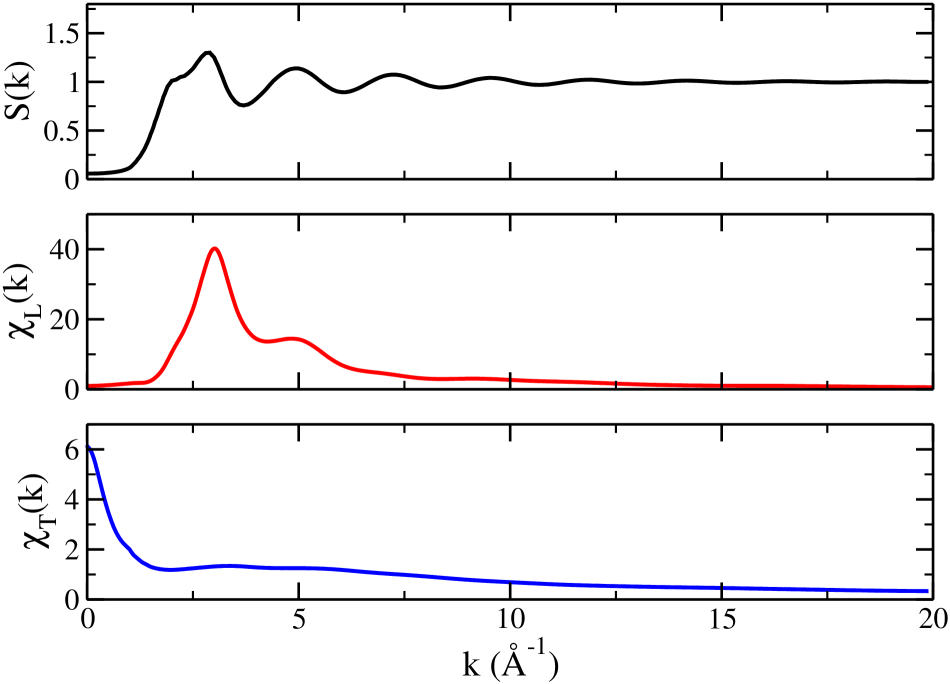
Figure 1: Structure factor and longitudinal and transverse dielectric susceptibility for SPC/E water computed according to the formulas in Ref [48]

$S^{-1}(r)$ and $\chi_{L,T}^{-1}(r)$ are defined as the Fourier transforms of the inverse of the structure factor $S(k)$ and longitudinal and transverse electric susceptibility $\chi_{L}(k)$ and $\chi_{T}(k)$, which may be obtained either from experimental data or by simulations through the correlation of the molecular density fluctuations and of the longitudinal and transverse polarisation vector fluctuations[45, 46, 47, 48]. We have computed these quantities for SPC/E water [49] using the k-space method described by Bopp et al[47, 48]; see Fig. 1. The dielectric susceptibilities are related to the longitudinal and transverse dielectric constants through $\chi_{L}(k)=1-1/\epsilon_{L}(k)$ and $\chi_{T}(k)=(\epsilon_{T}(k)-1)/4\pi$. Their very small k behavior, impaired in simulation by finite size effects, can thus be extrapolated using the macroscopic value of the dielectric constants $\epsilon_{L}(0)=\epsilon_{T}(0)=71$[50].

Note that in eqn S0.Ex6 the longitudinal polarization term can be also written as a charge-charge interaction term involving the bound charge density $\rho_{c}(\mathbf{r})=-\nabla\cdot\mathbf{P}(\mathbf{r})$ (that would also include the free charges in the case of a ionic solution). Note also that we have neglected the density-polarisation correlations which we verified to be very small in water. The negative terms in eqn S0.Ex6 stand for the linearized translational and orientational entropy, whereas the last term is the unknown correction term that contains supposedly all orders in $\Delta n(\mathbf{r})$ and $\mathbf{P}(\mathbf{r})$ higher that 2.

As will be seen below, the functional with ${\cal F}_{cor}=0$ tends to underestimate the tetrahedral order in the vicinity of the solute atomic sites giving rise to H-bonds with the solvent. Such defect was also present in our previous MDFT functional, involving the full angular-dependent c-functions in the excess functional[39]. To correct it, we introduce as before a short-range three-body potential term borrowed from the coarse-grained water model of Molinero et al. for water and ions in water[51, 52] that enforces some tetrahedral order around all atomic sites $k$ susceptible to give a H-bond interaction

$${\cal F}_{cor}[n(\mathbf{r})] = \frac{1}{2}k_{B}T\sum_{k}[\lambda_{k}^{1}\int d\mathbf{r}_{2}d\mathbf{r}_{3}\,f_{k}(r_{k2})\,f_{k}(r_{k3})(\frac{\mathbf{r}_{k2}\cdot\mathbf{r}_{k3}}{r_{k2}r_{k3}}-\cos\theta_{0})^{2}\,n(\mathbf{r}_{2})\,n(\mathbf{r}_{3})$$ (16)

$$+ \lambda_{k}^{2}\int d\mathbf{r}_{2}d\mathbf{r}_{3}f_{k}(r_{k2})\,f_{w}(r_{23})(\frac{\mathbf{r}_{k2}\cdot\mathbf{r}_{23}}{r_{k2}r_{23}}-\cos\theta_{0})^{2}\,n(\mathbf{r}_{2})\,n(\mathbf{r}_{3})],$$

with $r_{ki}=|\mathbf{r}_{i}-\mathbf{R}_{k}|$. The two terms describe three-body H-bonding to the the first and second water solvation shell, respectively. $f_{k}(r)$ and $f_{w}(r)$ are the short-range functions introduced by DeMille and Molinero for ion-water and water-water contributions. Their systematic parametrization, as well as the choice of the strength parameters $\lambda_{k}^{1},\lambda_{k}^{2}$, were alluded to in Ref. [39]. For simplicity, we have selected below the values $k_{B}T\lambda_{k}^{1}=k_{B}T\lambda_{k}^{2}=75$ kJ/mol for ionized H-bonding sites, and 50 kJ/mol for neutral ones, whatever their chemical nature.

We note finally that the above functional 12-S0.Ex6 (with ${\cal F}_{cor}=0$) can be shown to be equivalent to the generic dipolar functional introduced in Refs [35, 37] if the molecular polarization density is restricted to dipolar order in eqn 8, such that $\mathbf{P}(\mathbf{r})=\mu_{0}\int d\Omega\,\mathbf{\Omega}\,{\rho\left({\mathbf{r}},\Omega\right)}$. The present work can thus be viewed as a generalization of Refs [35, 37] to a Stockmayer-like multipolar solvent.

Implementation and results. The functional defined by eqs 12 to S0.Ex6 can be minimized in the presence of the external potential by discretizing ${\rho\left({\mathbf{r}},\Omega\right)}$ on a position and orientation grid. The minimization is performed in fact with respect to a ”fictitious wave function”, $\Psi(\mathbf{r},\Omega)=\rho(\mathbf{r},\Omega)^{1/2}$, in order to prevent the density from becoming negative in the logarithm. The position are represented on a 3D-grid with typically 3-4 points per Angstrom whereas the orientations are discretized using a Lebedev grid (yielding the most efficient angular quadrature for the unit sphere[53]) for $\theta,\phi$, the orientation of the molecule $C2v$ axis, and a regular grid for the remaining angle $\psi$ (from $0$ to $\pi$). We use typically $N_{\Omega}=12\times 3$ angles. The calculation begins with the tabulation of the external Lennard-Jones potential $\phi_{n}(\mathbf{r})$, and external electric field $\mathbf{E}_{c}(\mathbf{r})$. The latter is computed by extrapolating the solute charges on the grid and solving the Poisson equation. The molecular dipole function $\boldsymbol{\mu}(\mathbf{k},\Omega)$ is also precomputed in k-space. At each minimization cycle, ${\rho\left({\mathbf{r}},\Omega\right)}$ is Fourier transformed to get $\rho(\mathbf{k},\Omega)$, which is integrated over angles to get $n(\mathbf{k})~{}=~{}\int d\Omega\,\rho(\mathbf{k},\Omega)$ and $\mathbf{P}(\mathbf{k})=\int d\Omega\,\boldsymbol{\mu}(\mathbf{k},\Omega)\rho(\mathbf{k},\Omega)$, as well as its longitudinal and transverse components defined by eqn 15. The non-local excess terms in S0.Ex6 are computed in k-space and so are the gradients with respect to $\rho(\mathbf{k},\Omega)$; those are then back-transformed to r-space. The three-body contribution can be expressed as a sum of one-body terms and computed efficiently in r-space. For minimization, we used the L-BFGS quasi-Newton optimization routine[54] which requires as input at each cycle free energy and gradients. The calculation are performed on a standard workstation or laptop. The convergence turns out to be fast, requiring at most 25-30 iterations, so that despite the important number of FFT’s be handled at each step ($2\times N_{\Omega}$)[55], one complete minimization takes only a few minutes on a single processor. The computation of identical quantities using molecular dynamics simulations requires $10^{2}-10^{3}$ times more computer time[40, 41].

To describe water, we have chosen the SPC/E model[49] which defines both the external potential in eqs 10-11 and the structure factor and dielectric susceptibilities of equation S0.Ex6. Functional minimization was performed in the presence of different solutes placed the center of cubic box of size $L=25\,\AA$, with $80^{3}$ grid points. In figure 2, we display the ion-oxygen pair distribution functions obtained by MDFT minimization around two representative monovalent ions and compare them to the corresponding curves generated by molecular dynamics simulations using a similar box size. In the straight homogeneous reference fluid approximation, $F_{corr}=0$ in eqn S0.Ex6, it appears as in Ref. [39] that the first peak exhibits the correct position and width but is overestimated in height, whereas the second peak is misplaced; this later deficiency points to a lack of tetrahedral order. Those features are well corrected by inclusion of the three-body term of eqn 16. Identical comparisons are carried out in figure 3 for a SPC/E water molecule dissolved in our MDFT water model, and in figure 4 for a N-methyl-acetamide molecule (NMA: CH₃NHCOCH₃), the paradigm for a peptide bond chemical motif. Three-body contributions were added for the O and N sites with the parameters given in the previous section, the H-atoms being included implicitly in the associated heavy atom. The MDFT approach is able to provide not only pair distribution functions, but also the full three-dimensional solvent structure; this is illustrated for each molecule by an image of the surrounding three-dimensional water density. For water in water, the expected tetrahedral, four-fold coordination appears clearly, as does the fine structuring of water around the C=O and N-H bonds of NMA.

The purpose of this note was to derive a refined version of MDFT that is based on two natural physical fields, the particle density and polarization density, and on three simple, measurable bulk water properties. It was shown also that an efficient three-dimensional numerical implementation can be carried out. The next step will be the application of this new formalism to the hydration of complex molecular solutes, such as the atomistically-resolved clay surfaces considered in Ref. [41] with a reduced dipolar water model, or to the hydration of biological molecules. We will focus also on a systematic study of the performance of our novel MDFT scheme for the accurate prediction of molecules hydration free energies, in addition to the microscopic hydration structure.

Acknowledgments
The authors acknowledge financial support from the Agence Nationale de la Recherche under grant ANR-09-SYSC-012. DB acknowledges many thorough discussions about DFT with Rosa Ramirez and Shuangliang Zhao.

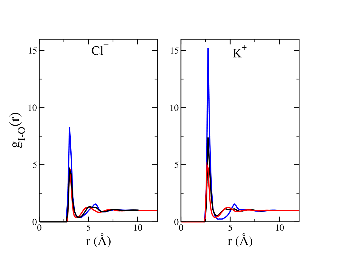
Figure 2: Ion-oxygen pair distribution functions for chloride and potassium ions in SPC/E water computed by MD (red lines) or MDFT without (blue lines) or with the three body term of eqn 16 (black lines)

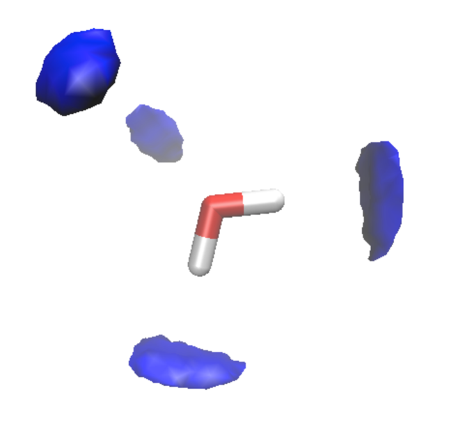
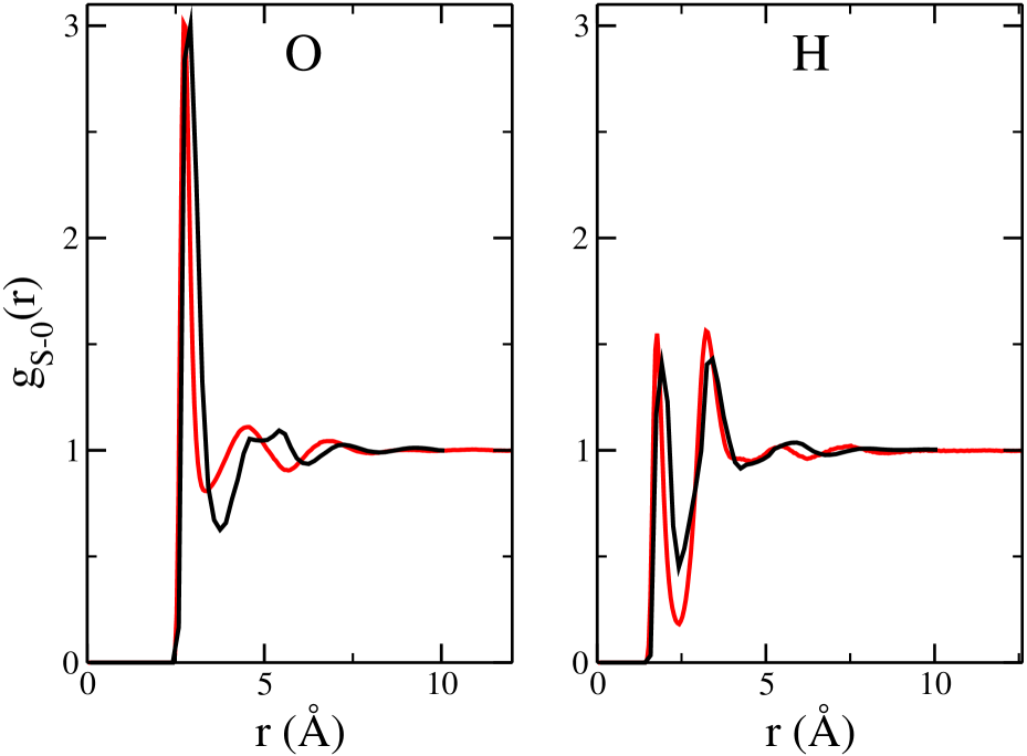
Figure 3: Top: Isosurface of high water density ($n(\mathbf{r})=3n_{0}$) around a tagged SPC/E water molecule as determined by MDFT. Bottom: Corresponding site-oxygen pair distribution functions computed by MD (red lines) or MDFT (black lines).

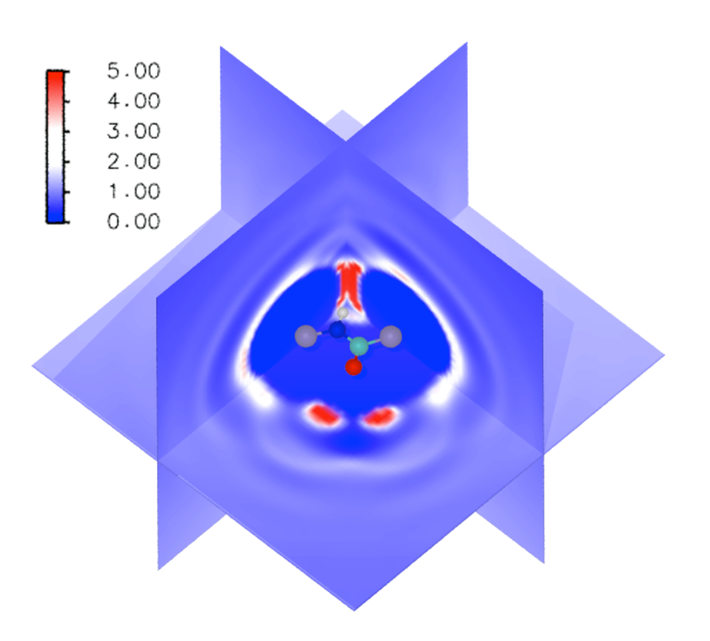
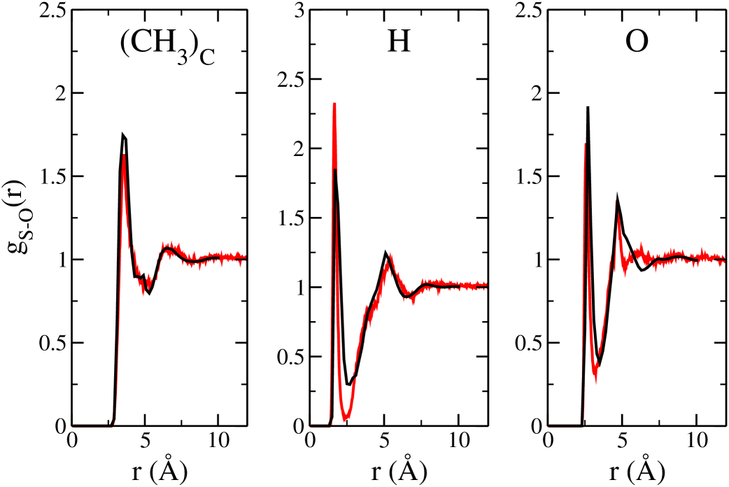
Figure 4: Top: Three-dimensional water density around a N-methyl-acetamide molecule obtained by MDFT. Bottom: A selection of solute site-oxygen pair distribution functions computed by MD (red lines) or MDFT (black lines).

References

- [1] Hansen, J. P.; McDonald, I. R. Theory of Simple Liquids; Academic Press: London, 1989.
- [2] Gray, C. G.; Gubbins, K. E. Theory of Molecular Fluids, Volume 1: Fundamentals; Clarendon Press: Oxford, 1984.
- [3] Chandler, D.; Hendersen, H. Optimized Cluster Expansions for Classical Fluids II- Theory of Molecular Liquids. J. Chem. Phys. 1972, 57, 3275–3276.
- [4] Hirata, F.; Rossky, P. J. An Extended RISM Equation for Molecular Polar Fluids. Chem. Phys. Lett. 1981, 83, 329–334.
- [5] Hirata, F.; Pettitt, B. M.; Rossky, P. J. Application of an Extended RISM Equation to Dipolar and Quadrupolar Fluids. J. Chem. Phys. 1982, 77, 509–520.
- [6] Reddy, G.; Lawrence, C. P.; Skinner, J. L.; Yethiraj, A. Liquid State Theories for the Structure of Water. J. Chem. Phys. 2003, 119, 13012–13016.
- [7] Dyer, K. M.; Perkyns, J. S.; Pettitt, B. M. A Site-Renormalized Molecular Fluid Theory. J. Chem. Phys. 2007, 127, 194506–194506-14.
- [8] Dyer, K. M.; Perkyns, J. S.; Stell, G.; Pettitt, B. M. A Molecular Site-Site Integral Equation that Yields the Dielectric Constant. J. Chem. Phys. 2008, 129, 104512–104512-9.
- [9] Blum, L.; Torruella, A. J. Invariant Expansion for 2-Body Correlations I- Thermodynamic Functions, Scattering, and Ornstein-Zernike Equation. J. Chem. Phys. 1972, 56, 303–310.
- [10] Blum, L. Invariant Expansion II- Ornstein-Zernike Equation for Nonspherical Molecules and an Extended Solution to Mean Spherical Model. J. Chem. Phys. 1972, 57, 1862–1869.
- [11] Patey, G. N. Integral-Equation Theory for Dense Dipolar Hard-Sphere Fluid. Mol. Phys. 1977, 34, 427–440.
- [12] Fries, P. H.; Patey, G. N. The Solution of the Hypernetted-Chain Approximation for Fluids of Nonspherical Particles - a General Method with Application to Dipolar Hard-Spheres. J. Chem. Phys. 1985, 82, 429–440.
- [13] Richardi, J.; Fries, P. H.; Krienke, H. The Solvation of Ions in Acetonitrile and Acetone: A Molecular Ornstein-Zernike Study. J. Chem. Phys. 1998, 108, 4079–4089.
- [14] Richardi, J.; Millot, C.; Fries, P. H. A Molecular Ornstein-Zernike Study of Popular Models for Water and Methanol. J. Chem. Phys. 1999, 110, 1138–1147.
- [15] Evans, R. Nature of the Liquid-Vapor Interface and Other Topics in the Statistical-Mechanics of Nonuniform, Classical Fluids. Adv. Phys. 1979, 28, 143–200.
- [16] Evans, R. In Henderson, D., Ed., Fundamental of Inhomogeneous Fluids, New York, 1992. Marcel Dekker.
- [17] Wu, J.; Li, Z. Density Functional Theory for Complex Fluids. Ann. Rev. Phys. Chem. 2007, 58, 85–112.
- [18] Chandler, D. Gaussian Field Model of Fluids with an Application to Polymeric Fluids. Phys. Rev. E 1993, 48, 2898–2905.
- [19] Lum, K.; Chandler, D.; Weeks, J. D. Hydrophobicity at Small and Large Length Scales. J. Phys. Chem. B 1999, 103, 4570–4577.
- [20] ten Wolde, P. R.; Sun, S. X.; Chandler, D. Model of a Fluid at Small and Large Length Scales and the Hydrophobic Effect. Phys. Rev. E 2002, 65, 011201–011201-9.
- [21] Coalson, R. D.; Duncan, A. Statistical Mechanics of a Multipolar Gas: A Lattice Field Theory Approach. J. Phys. Chem. 1996, 100, 2612–2620.
- [22] Gray, C. G.; Gubbins, K. E.; Joslin, C. J. Theory of Molecular Fluids, Volume2: Applications; Clarendon Press: Oxford, 2011.
- [23] Ravikovitchand, P.; Neimark, A. Density Functional Theory Model of Adsorption on Amorphous and Microporous Silica Materials. Langmuir 2006, 22, 11171–11179.
- [24] Gor, G. Y.; Neimark, A. Adsorption-Induced Deformation of Mesoporous Solids: Macroscopic Approach and Density Functional Theory Langmuir 2011, 27, 6926–6931.
- [25] Wu, J. Density Functional Theory for Chemical Engineering: From Capillarity to Soft Materials. AIChE Journal 2006, 52, 1169–1193.
- [26] Beglov, D.; Roux, B. An Integral Equation to Describe the Solvation of Polar Molecules in Liquid Water. J. Phys. Chem. B 1997, 101, 7821–7826.
- [27] Kovalenko, A.; Hirata, F. Three-Dimensional Density Profiles of Water in Contact with a Solute of Arbitrary Shape; a RISM Approach. Chem. Phys. Lett. 1998, 290, 237–244.
- [28] F. Hirata, E. Molecular Theory of Solvation; Kluwer Academic Publishers, Dordrecht, 2003.
- [29] Yoshida, N.; Imai, T.; Phongphanphanee, S.; Kovalenko, A.; Hirata., F. Molecular Recognition in Biomolecules Studied by Statistical-Mechanical Integral-Equation Theory of Liquids. J. Phys. Chem. B 2009, 113, 873–886.
- [30] Kloss, T.; Kast, S. M. Treatment of Charged Solutes in Three-Dimensional Integral Equation Theory. J. Chem. Phys. 2008, 128, 134505–134505-7.
- [31] Kloss, T.; Heil, J.; Kast, S. M. Quantum Chemistry in Solution by Combining 3d-Integral Dquation Theory with a Cluster Embedding Approach. J. Phys. Chem. B 2008, 112, 4337–4343.
- [32] Azuara, C.; Lindahl, E.; Koehl, P. Pdb_hydro: Incorporating Dipolar Solvents with Variable dDnsity in the Poisson-Boltzmann Treatment of Macromolecule Electrostatics. Nucleic Ac. Res. 2006, 34, W38–W42.
- [33] Azuara, C.; Orland, H.; Bon, M.; Koehl, P.; Delarue, M. Incorporating Dipolar Solvents with Variable Density in Poisson-Boltzmann Electrostatics. Biophys. J. 2008, 95, 5587–5605.
- [34] Varilly, P.; Patel, A. J.; Chandler, D. An Improved Coarse-Grained Model of Solvation and the Hydrophobic Effect. J. Chem. Phys. 2010, 134, 074109–074109-15.
- [35] Ramirez, R.; Gebauer, R.; Mareschal, M.; Borgis, D. Density Functional Theory of Solvation in a Polar Solvent: Extracting the Functional from Homogeneous Solvent Simulations. Phys. Rev. E 2002, 66, 031206–031206-8.
- [36] Ramirez, R.; Mareschal, M.; Borgis, D. Direct Correlation Functions and the Density Functional Theory of Polar Solvents. Chem. Phys. 2005, 319, 261–272.
- [37] Ramirez, R.; Borgis, D. Density Functional Theory of Solvation and its Relation to Implicit Solvent Models. J. Phys. Chem. B 2005, 109, 6754–6763.
- [38] Gendre, L.; Ramirez, R.; Borgis, D. Classical Density Functional Theory of Solvation in Molecular Solvents: Angular Grid Implementation. Chem. Phys. Lett. 2009, 474, 366–370.
- [39] Zhao, S.; Ramirez, R.; Vuilleumier, R.; Borgis, D. Molecular Density Functional Theory of Solvation: From Polar Solvents to Water. J. Chem. Phys. 2011, 134, 194102–194102-13.
- [40] Borgis, D.; Gendre, D.; Ramirez, R. Molecular Density Functional Theory: Application to Solvation and Electron-Transfer Thermodynamics in Polar Solvents. J. Phys. Chem. B 2012, 116, 2504–2512.
- [41] Levesque, M.; Marry, V.; Rotenberg, B.; Jeanmairet, G.; Vuilleumier, R.; Borgis, D. Solvation of Complex Surfaces via Molecular Density Functional Theory. J. Chem. Phys. 2012, 137, 224107–224107-8.
- [42] Zhao, S.; Jin, Z.; Wu, J. A new theoretical method for rapid prediction of solvation free energy in water. J. Phys. Chem. B 2011, 115, 6971–6975.
- [43] Zhao, S.; Jin, Z.; Wu, J. Correction to “New Theoretical Method for Rapid Prediction of Solvation Free Energy in Water”. J. Phys. Chem. B 2011, 115, 15445–15445.
- [44] Levesque, M.; Vuilleumier, R.; Borgis, D. Scalar Fundamental Measure Theory for Hard Spheres in Three Dimensions. Application to Hydrophobic Solvation. J. Chem. Phys. 2012, 137, 034115–034115-9.
- [45] Raineri, F. O.; Resat, H.; Friedman, H. L. Static Longitudinal Dielectric Function of Model Molecular Fluids. J. Chem. Phys. 1992, 96, 3068–3084.
- [46] Raineri, F. O.; Friedman, H. L. Static Transverse Dielectric Function of Model Molecular Fluids. J. Chem. Phys. 1993, 98, 8910–8918.
- [47] Bopp, P. A.; Kornyshev, A. A.; Sutmann, G. Static Nonlocal Dielectric Function of Liquid Water. Phys. Rev. Lett. 1996, 76, 1280–1283.
- [48] Bopp, P. A.; Kornyshev, A. A.; Sutmann, G. Frequency and Wave-Vector Dependent Dielectric Function of Water: Collective Modes and Relaxation Spectra. J. Chem. Phys. 1998, 109, 1939–1958.
- [49] Berendsen H. J. C.; Grigera J. R.; Straatsma T. P. The Missing Term in Effective Pair Potential. J. Phys. Chem. 1987, 91, 6269–6271.
- [50] Kusalik P. G.; Svishchev I. M. The spatial Structure in Liquid Water Science 1994, 265, 1219–1221.
- [51] Molinero, V.; Moore, E. B. Water Modeled as an Intermediate Element between Carbon and Silicon. J. Phys. Chem. B 2009, 113, 4008–4016.
- [52] DeMille, R. C.; Molinero, V. Coarse-Grained Ions without Charges: Reproducing the Solvation Structure of NaCl in Water. J. Chem. Phys. 2009, 131, 034107-034107–16.
- [53] Lebedev, V. I.; Laikov D. N. A Quadrature Formula for the Sphere of the 131st Algebraic Order of Accuracy. Dokl. Math. 1999, 59, 477–481.
- [54] Byrd, R. H.; Lu, P.; Nocedal, J. A Limited Memory Algorithm for Bound Constrained Optimization. SIAM J. Scient. Stat. Comp. 1994, 16, 1190–1208.
- [55] Frigo M. and Johnson S. G. FFTW: a free collection of fast fourier transforms routines in C. Available at the FFTW home page: http://theory.lcs.mit.edu/ fftw.