Non-congruence of the nuclear liquid-gas and deconfinement phase transitions

Abstract

First order phase transitions (PTs) with more than one globally conserved charge, so-called non-congruent PTs, have characteristic differences compared to congruent PTs (e.g., dimensionality of phase diagrams, location and properties of critical points and endpoints). In the present article we investigate the non-congruence of the nuclear liquid-gas PT at sub-saturation densities and the deconfinement PT at high densities and/or temperatures in Coulomb-less models, relevant for heavy-ion collisions and neutron stars. For the first PT, we use the FSUgold relativistic mean-field model and for the second one the relativistic chiral SU(3) model. The chiral SU(3) model is one of the few models for the deconfinement PT, which contains quarks and hadrons in arbitrary proportions (i.e. a “solution”) and gives a continuous transition from pure hadronic to pure quark matter above a critical point. The study shows the universality of the applied concept of non-congruence for the two PTs with an upper critical point, and illustrates the different typical scales involved. In addition, we find a principle difference between the liquid-gas and the deconfinement PTs: in contrast to the ordinary Van-der-Waals-like PT, the phase coexistence line of the deconfinement PT has a negative slope in the pressure-temperature plane. As another qualitative difference we find that the non-congruent features of the deconfinement PT become vanishingly small around the critical point.

I Introduction

Nuclear matter is expected to undergo two different major phase transitions (PTs): the liquid-gas phase transition (LGPT) of nuclear matter at sub-saturation densities and moderate temperatures and the deconfinement and chiral symmetry restoration PT at high densities and/or temperatures. For convenience we will call the latter also the quark hadron phase transition (QHPT) or QCD PT. These two PTs are actively discussed in the contexts of heavy-ion collisions and astrophysics. The latter includes the interior of compact stars, i.e., neutron stars (NS) or so-called hybrid stars which have quark matter in their core.

Various effective models for nuclear matter which are constrained by properties of nuclei have shown that the LGPT of bulk uniform nucleonic matter, i.e. consisting of neutrons and protons without Coulomb interactions, is of first order (see Refs. Fiorilla et al. (2012); Somà and Bożek (2009) for two recent examples of microscopic models). Furthermore, there is also experimental evidence for this from intermediate-energy heavy-ion collisions Pochodzalla et al. (1995); Elliott et al. (2002); Bonnet et al. (2009). On the other hand, for smaller systems the LGPT is also found to have critical behavior Ma et al. (1997, 2005).

For the QHPT the situation is more uncertain. Ab-initio solutions of QCD exist only for very high densities and/or temperatures Kurkela et al. (2010a, b); Vuorinen (2003); Andersen et al. (2011a, b). Simulations on the lattice have shown that the QHPT is a smooth crossover at vanishing density. Unfortunately their use at finite densities is problematic because they suffer from the so-called “sign problem”. It is a numerical problem found in quantum mechanical systems of fermions which comes from the fact that at finite chemical potential the fermion determinant is complex (see Refs. Philipsen (2008); Fukushima and Sasaki (2013) and references therein for details). As a consequence, effective models for QCD matter have to be used, resulting in different varieties of possible QCD phase diagrams Blaschke et al. (2005); Baym et al. (2008); Powell and Baym (2012); Yamamoto et al. (2007); Yamamoto (2008); Abuki et al. (2010); Kneur et al. (2010); Steinheimer et al. (2010); Steinheimer et al. (2011a); Lourenco et al. (2011); Lourenço et al. (2012); McLerran and Pisarski (2007); Herbst et al. (2011); Hatsuda et al. (2006); Bratovic et al. (2013); Sasaki and Mishustin (2010); Andronic et al. (2010); Mintz et al. (2013). Many of these models predict that the QCD PT at low temperatures is of first order like the LGPT, but some also predict a cross-over transition in this regime. In the present investigation we assume that both the LGPT and the QHPT are of first order, and concentrate on the detailed thermodynamic aspects of the two phase transitions and especially their non-congruent features.

A non-congruent phase transition (NCPT) naturally occurs for a first-order PT with more than one globally conserved charge. In this case it becomes possible that the local concentrations of the charges vary during a phase transformation, i.e., the crossing of a phase-coexistence region. This leads to qualitative differences compared to congruent PTs. Consider for example a phase diagram in the temperature–pressure plane. For a given temperature, a NCPT occurs over a range of pressure, related to a range of local concentrations of the charges. For a congruent PT, the equilibrium conditions can only be fulfilled at a single value of the pressure for each temperature. As we will show, also other characteristics of PTs depend on the number of globally conserved charges. It is the main scope of the present article to identify and discuss these non-congruent features.

As will be explained below, isospin symmetric matter is an “azeotrope”, which means that it leads to a congruent PT even though it consists of more than one globally conserved charge. Consequently, the non-congruent features only become visible for an isospin asymmetric system, and are thus highly related to the isospin asymmetry. Phase diagrams of isospin asymmetric matter are of extreme importance for the complete understanding of QCD and nuclear matter. They are highly related to the symmetry energy, as explained, e.g., in Refs. Di Toro et al. (2011, 2006); Zhang and Jiang (2013). Such studies are also used to analyze the effect of model parameters on the QCD phase diagram Shao et al. (2011a); Liu et al. (2011); Shao et al. (2011b); Blaschke et al. (2013). The effect of different isospin/charge assumptions has been studied already extensively in the literature for the LGPT Baym et al. (1971); Lattimer and Ravenhall (1978); Barranco and Buchler (1980); Müller and Serot (1995); Ducoin et al. (2006); Zhang and Jiang (2013); Lavagno and Pigato (2012), and also experimentally Sfienti et al. (2009); McIntosh et al. (2013), and for the QHPT Müller (1997); Shao et al. (2011a, b) as well. Some authors Müller and Serot (1995); Müller (1997); Tatsumi et al. (2011); Aguirre (2012); Lavagno and Pigato (2012) have stated that the LGPT and QHPT changes from first to second order (according to the Ehrenfest classification) if one goes to an asymmetric system. This was concluded from the non-standard behavior of thermodynamic quantities during an isothermal crossing of the two-phase region. One of the main statements of the present paper is that this non-standard behavior in asymmetric matter is the typical manifestation of a non-congruent first-order PT.

In the present article, the LGPT and the QHPT are studied for the scenarios of heavy-ion collisions of symmetric and asymmetric nuclei. For the QHPT, we are also investigating the scenario of the interior of a neutron, respectively hybrid star. For this purpose we use a relativistic chiral SU(3) effective model. This model predicts that both the LG and the QCD PT at low temperatures are of first order. Due to technical reasons, the chiral SU(3) model is applied only for the QHPT. For the description of the LGPT we apply the FSUgold relativistic mean-field model. Even using only one selected theoretical model for the QHPT and one for the LGPT, our main conclusions are to some extent model-independent, because the applied thermodynamic concepts are rather universal.

The structure of this article is as follows: in Sec. II we discuss various aspects of (non-)congruence of PTs in detail. In Sec. III we describe the effective model used for the calculations of the LGPT, the FSUgold equation of state (EOS). In Sec. IV we continue with the description of the chiral SU(3) model for the QHPT. In Sec. V we specify our thermodynamic model and setup used for the two PTs and the different physical systems. In Sec. VI we analyze and compare in detail the results for the different scenarios, with a focus on the structure of the resulting phase diagrams and the non-congruent features. In Sec. VII we summarize our main findings and draw conclusions.

II Congruence/non-congruence of phase transitions

II.1 Definition of non-congruence

The term “non-congruent” (or “incongruent”) phase transition (NCPT) denotes the situation of phase coexistence of two (or more) macroscopic phases with different chemical compositions (see the IUPAC definition Clarke et al. (1994) and Ref. Iosilevskiy (2010)). Such systems are also called “binary”, “ternary”, etc., in contrast to “unary” systems. NCPTs are well known since long ago in many terrestrial applications as a particular type of PTs (regardless of the term), e.g. in low-temperature solution theory (see e.g. Ref. Landau and Lifshitz (1969)), in the theory of simple liquid mixtures of hydrocarbons (see e.g. Ref. Reid and Sherwood (1966)), or in the theory of crystal-fluid and crystal-crystal phase diagrams in chemical compounds. NCPTs are also known in nuclear physics Barranco and Buchler (1980), in heavy-ion physics Greiner et al. (1987), and also in the physics of compact stars Glendenning (1992) since quite some time, but the term “non-congruent” has been introduced to these areas of physics only recently (see below).

The variants of terrestrial NCPT which are the closest ones to LGPT and QHPT discussed in the present article, are PTs in high-temperature, chemically reacting and partially ionized plasmas—typical products of extremely heated chemical compounds. NCPTs were studied thoroughly for high-temperature uranium-oxygen systems during hypothetical “severe accidents” in the framework of nuclear reactor safety problems Iosilevskiy et al. (2001, 1999, 1997, 1999); Ronchi et al. (2004); Iosilevskiy (2011); Iosilevskiy et al. (2003). The universal nature of this type of PT and its applicability for most astrophysical objects was claimed and illustrated in Ref. Iosilevskiy et al. (2003), using the examples of (hypothetical) plasma PTs in the interiors of Jupiter and Saturn, brown dwarfs, and extrasolar planets. The identification that most PTs in neutron stars are non-congruent, in particular for the QHPT in hybrid stars, was claimed first at several conferences by I.I. and then published recently in Ref. Iosilevskiy (2010). Nowadays, the term “non-congruent” PT is already used in the astrophysical literature Tatsumi et al. (2011); Maruyama and Tatsumi (2012). Our theoretical description of the LGPT and QHPT as non-congruent phase transitions in the present study is based essentially on experience from terrestrial applications.

It should be noted that in the above standard terrestrial definition of NCPTs, different ionized states of atoms or molecules are not relevant for the possible non-congruence, but only the number of chemical elements. The additional degree of freedom of ionization does not count in the definition because one deals with phase coexistence of two electroneutral macroscopic phases (or a mixture of several electroneutral macroscopic fragments). For macroscopic phases, Coulomb interactions automatically lead to local charge neutrality, and thereby suppress this degree of freedom. Conversely, for all thermodynamic systems in the present paper, including those corresponding to matter in neutron stars, Coulomb interactions are not taken into account explicitly, in spite of the presence of charged species (protons, quarks, leptons, etc.). This is what we call a “Coulomb-less” model description. In such a Coulomb-less approach positive and negative charges (e.g., nuclei and electrons) play the role of different chemical elements. In nuclear matter the abundance of chemical elements is typically not conserved, but only some generalized “charges” like baryon number, electric charge, and possibly also isospin or strangeness. The generalization of the definition of non-congruence to first-order PTs in dense nuclear matter, described as Coulomb-less systems with more than one conserved charge, is thus obvious: phase coexistence of two (or more) macroscopic phases with different composition of the charges, including electric charge.

There is a famous example from the context of neutron stars which illustrates the definition of non-congruence: in beta-equilibrated, cold neutron stars baryon number and total net electric charge (which has to be zero) are two conserved charges. There are two typical choices for the treatment of charge neutrality for PTs of macroscopic phases within the Coulomb-less approximation. In the first case, one assumes local charge neutrality, with zero net charge in both phases, and thus one obtains a congruent PT of a unary system. Because here the congruence is enforced by the requirement of local charge neutrality we call it more specifically to be a “forced-congruent” PT as proposed in Iosilevskiy (2010). In astrophysics this scenario is usually called the “Maxwell-PT”, which is then used as a synonym for congruent phase transitions in general. In the second case one assumes global charge neutrality. In this case the two coexisting phases will have electric charge concentrations of opposite sign. Consequently the system is binary and the PT is non-congruent Glendenning (1992). In astrophysics this is often called the “Gibbs-PT”, and again taken as a synonym for non-congruent PTs in general. The classification with respect to “Gibbs” or “Maxwell” of matter in supernovae or proto-neutron stars with possibly trapped neutrinos was given in Ref. Hempel et al. (2009). Nuclear matter in heavy-ion collisions also has more than one conserved charge, namely net baryon number, net electric charge and also net weak flavor, respectively isospin, due to the fast timescales involved. Thus Coulomb-less PTs in heavy-ion collisions will in general also be non-congruent, see also Ref. Greiner et al. (1987). Ref. Sissakian et al. (2006) addresses experimental consequences of the QHPT as a non-congruent PT. The previous arguments are valid for both PTs, LGPT and QHPT, just the typical scales involved and the quantitative behavior is different.

II.2 Coulomb interactions

As mentioned before, it should be stressed that for all thermodynamic systems in the present paper we are using a “Coulomb-less” model description. Also, surface effects are neglected in our work. As a consequence, the two-phase mixtures at equilibrium (i.e., not metastable) within the two-phase regions are always described as coexistence of two macroscopic phases.

The simplification of Coulomb-less is to some extent reasonable for the theoretical description of relativistic heavy-ion collisions, where one has a net electric charge but Coulomb energies are small compared to the typical collision energies. Furthermore, the long-range nature of Coulomb forces could be ignored in view of the small size of the ensemble of heavy-ion collisions products. However, for the same reason it is questionable whether the thermodynamic limit is fulfilled or not Chomaz and Gulminelli (2005). On the other hand, for the description of nuclears clusters appearing in the nuclear liquid-gas PT of low-energy heavy-ion collsions, Coulomb and surface energies are in fact crucial. Nevertheless, the bulk Coulomb-less treatment gives useful insight into the main characteristics of the PT.

Matter in neutron stars has to be overall charge neutral in order to be gravitationally bound. In this case, Coulomb interactions and corresponding surface effects can be included in a more detailed mesoscopic description, leading to structured mixed phases. Usually these phases with finite-size substructures are called the “pasta phases” Ravenhall et al. (1983); Maruyama et al. (2005); Newton and Stone (2009); Watanabe and Maruyama (2011); Avancini et al. (2012); Na et al. (2012) or “pasta plasma” Iosilevskiy (2010). The classification with respect to non-congruence of these scenarios is somewhat still an open question Iosilevskiy (2010). In a strict thermodynamic sense, the state of matter in such mesoscopic calculations should not be seen as the two-phase coexistence of a first-order PT, but rather as a sequence of single phases with non-uniform substructure.

A very low surface tension between the two phases (see Refs. Pinto et al. (2012); Mintz et al. (2013) for possible calculations of the surface tension) would lead to a highly dispersed charged and non-soluble mixture of micro-fragments of one phase into the other, a mixed phase, which also could be called a charged “emulsion”. We remark that very often in the astrophysical literature, matter in the two-phase coexistence region of any PT, including those in neutral systems, is generally said to be in a “mixed phase”. We think it is more accurate to denote this as a “two-phase mixture” and to reserve the term “mixed phase” only for the state of matter obtained in the mesoscopic description of PTs in Coulomb systems with a low surface tension, as described above.

Without a detailed mesoscopic treatment, the effect of Coulomb interactions in NSs can be estimated by different assumptions for charge neutrality Heiselberg et al. (1993); Maruyama et al. (2008); Pagliara et al. (2010); Yasutake et al. (2012), which we will use in the present study. The assumption of local charge neutrality, used in the “Maxwell-PT” which was already introduced above, corresponds to the limit of an infinitely high surface tension between the two phases. In terrestrial plasmas, phase equilibrium of locally charge neutral phases with Coulomb forces is denoted more accurately as the Gibbs-Guggenheim conditions for phase equilibrium, see e.g. Ref. Iosilevskiy (2010). Conversely, the usage of global charge neutrality (GCN) for macroscopic phases in a Coulomb-less approach can be seen as an approximation for the case of a vanishing surface tension in the mesoscopic description. In astrophysics, this is typically called the “Gibbs-PT” Glendenning (1992).

II.3 Characteristics of non-congruent PT

It was shown in Refs. Iosilevskiy et al. (2001, 1999, 1997, 1999); Ronchi et al. (2004); Iosilevskiy (2011); Iosilevskiy et al. (2003); Iosilevskiy (2010); Barranco and Buchler (1980); Greiner et al. (1987); Glendenning (1992); Müller and Serot (1995) and many others, and it will also be shown below, that non-congruency significantly changes the properties of all PTs, namely: (A) Significant impact on the phase transformation dynamics, i.e., a strong dependence of the PT parameters on the rapidity of the transition Ronchi et al. (2004). (B) The thermodynamics of PTs becomes more complicated. The essential changes include: (1) significant change in properties of the singular points (critical point first of all) and separation of critical point and endpoints, such as temperature endpoint, pressure endpoint, etc. (2) significant change in the scale of two-phase boundaries in extensive thermodynamic variables (say $P$-$V$, $V$-$T$, $H$-$T$, etc.) and even in topology of all two-phase boundaries in the space of all intensive thermodynamic variables, i.e., pressure, temperature, specific Gibbs free energy etc. Note, that this is valid for both types of PTs: with and without a critical point (e.g. gas-liquid-like PT and crystal-fluid-like PT, correspondingly). One of the most remarkable consequences of the non-congruence in NCPT is the appearance of a two-dimensional “banana-like” region instead of the well-known one-dimensional $P$-$T$ saturation curve for ordinary (congruent) PTs (see Fig. 1 in Ref. Iosilevskiy (2010)). The same should be expected in the plane of the widely used pair of variables: temperature - baryon chemical potential (see below). (3) Closely connected to this is the significant change of the behavior in the two-phase region: i.e. isothermal and isobaric crossings of the two-phase region do not longer coincide. The isothermal NCPT starts and finishes at different pressures, while the isobaric NCPT starts and finishes at different temperatures. Basically, the pressure on an isotherm is monotonically increasing with density.

Aspect (3) of NCPTs is well studied in the context of neutron stars Glendenning (1992). Inside a neutron star, the pressure has to decrease monotonically with the radius. A congruent PT leads therefore to a spatial separation of the two coexisting phases, with a discontinuous jump in density and all extensive thermodynamic variables at the transition radius inside the neutron star. Conversely, for a NCPT a spatially extended two-phase coexistence region is present, with a continuous change of total density, total energy density, etc, throughout. We remark that for the LGPT there exist several works which also have discussed the other characteristic features of NCPTs and only used a partially different terminology, see, e.g., Refs. Barranco and Buchler (1980); Müller and Serot (1995); Lavagno and Pigato (2012). For the QHPT, the possible non-congruence has not been discussed in such detail as is done here.

Furthermore, even nowadays publications are still appearing which do not treat the thermodynamic aspects of non-unary phase transitions, i.e., the non-congruent features, in a proper way. For example aspect (3) sometimes led to the conclusion that one has a second-order PT according to the Ehrenfest classification, as e.g., in Refs. Müller and Serot (1995); Müller (1997); Tatsumi et al. (2011); Aguirre (2012); Lavagno and Pigato (2012). However, the two coexisting phases have different order parameters like densities, entropies, asymmetries, etc., and, most importantly for our purposes, different generalized “chemical” compositions. At the interface between the two macroscopic phases there is a discontinuous jump of the order parameter and thus the PT is still of first order. Also the first two aspects of (B) from above are sometimes overseen or neglected in the literature which means that the non-congruence is not fully taken into account (compare, e.g., with Ref. Fiorilla et al. (2012)).

II.4 Isospin symmetry, azeotrope

The isospin symmetry of strong forces plays an important role for the possible non-congruence of the LGPT and the QHPT. Independently of density and temperature, isospin symmetric nuclear matter always represents the state with the lowest thermodynamic potential (neglecting Coulomb interactions and assuming equal masses of protons and neutrons). Thus the isospin chemical potential is zero for symmetric nuclear matter. As a consequence, isospin does not appear as a relevant charge for symmetric nuclear matter because this degree of freedom is not explored, i.e. even in a first-order PT the involved phases remain symmetric. Therefore the LG and QH PTs remain congruent if the system is exactly symmetric and if no other globally conserved charge than baryon number is involved (see also Appendix B). This is called “azeotropic” behavior, denoted for a system with more than one conserved charge whose charge ratios cannot be changed by distillation for a certain azeotropic composition. The ensemble of such azeotropic points in the parameter space, e.g., for all temperatures, is called an azeotropic curve. Note that the isospin asymmetry of the hot state of matter in a heavy-ion collision experiment is mainly set by the initial charge to mass ratio $Z/A$ of the colliding nuclei, e.g., $Z/A\simeq 0.4$ in Au+Au collisions.

II.5 Unified EOS

As mentioned in point (1) in Section II.3, another consequence of non-congruent phase transitions is the possible emergence of critical points, which are different from the points of maximum temperature, pressure, or extremal chemical potential. To obtain such critical points and endpoints at all, it is necessary that both of the two involved phases are calculated with the same theoretical model (“unified” or “single” EOS approach). In other words, one has to use only one underlying many-body Hamilton operator. This is in contrast to a “two-EOS” approach, where two different EOS models are applied for the two phases in coexistence. Such a “two-EOS” description can have several short-comings, as it cannot contain critical points and endpoints (see Appendix A, and standard literature, e.g., Ref. Landau and Lifshitz (1969)) and it does not give a consistent description of meta-stable or unstable matter in the binodal, respectively spinodal regions, e.g., for a liquid-gas type PT. In summary, in the “unified” EOS approach both coexisting phases are presumed as isostructural (like gas and liquid) with a possible continuous transition from one phase into another, while in the two-EOS approach this is impossible.

Almost all studies of the LGPT are based on the unified EOS approach. This also applies for our investigation of the LGPT with the FSUgold relativistic mean-field model. Unified EOS approaches for the QHPT are usually either built with only hadrons or only quarks. Thus they do not give the expected degrees of freedoms for one of the two phases. Alternatively, often the two-EOS approach is applied for the QHPT (see, e.g., Ref. Müller (1997)) to have the right degrees of freedom. On the other hand this approach cannot contain all possible non-congruent features of the singular points, as explained above. The chiral SU(3) model used in the present study is one of the few unified-EOS approaches for the QHPT that contains hadronic as well as quark degrees of freedom. These can appear, in principle, in arbitrary proportions (solution-like mixture) with the interactions leading to the correct behavior for low, respectively high, densities and temperatures. See Refs. Steinheimer et al. (2011b, a) for another unified-EOS model that also contains hadronic and quark degrees of freedom. As another exception of a unified-EOS approach for the QHPT with the correct degrees of freedom there is the EOS of Ref. Randrup (2010), where the two-EOS approach is transformed into a one-EOS version with the use of a special spline-based interpolation procedure.

III FSUgold RMF model

For the LGPT of nucleonic matter we apply a relativistic mean-field (RMF) model. In principle, also the Chiral model could be used for this, as it also contains the LGPT Dexheimer and Schramm (2010). However, due to the different characteristic scales involved and for numerical reasons, we use a dedicated model for the LGPT which occurs at sub-saturation densities. We choose the FSUgold RMF parameterization Todd-Rutel and Piekarewicz (2005), because of its excellent description of matter around and below saturation density and because its neutron matter EOS is in agreement with recent experimental and observational constraints (see e.g. Ref. Lattimer and Lim (2012)). Its Lagrangian is based on the exchange of the isoscalar–scalar $\sigma$, the isoscalar–vector $\omega$ and the isovector–vector $\rho$ mesons between nucleons. Particular for FSUgold, also the coupling between the $\omega$ and the $\rho$ meson is included. This leads to a better description of nuclear collective modes, the EOS of asymmetric nuclear matter, and a different density dependence of the symmetry energy Piekarewicz (2007). The free parameters of the Lagrangian, the meson masses and their coupling constants, are determined by fits to experimental data, more specifically to binding energies and charge radii of a selection of magic nuclei.

The only baryonic degrees of freedom in FSUgold are neutrons and protons. For the typical densities and temperatures of the LGPT, hyperonic or quark degrees of freedom are not relevant. Because FSUgold considers only the “elementary” particles of the LGPT but not any compound objects, respectively bound complexes like light or heavy nuclei, it belongs to the class of so-called physical descriptions of PTs. In this description, all effects of bound complexes are presumed to be taken into account by the interactions (“non-ideality”) of the “elementary” particles (see, e.g., Ref. Ebeling et al. (1976)). However, for a more detailed description of the nuclear EOS like, e.g., used in simulations of core-collapse supernovae, the formation of nuclei and nuclear clusters has to be incorporated explicitly, see e.g., Refs. Shen et al. (1998); Typel et al. (2010); Botvina and Mishustin (2010); Hempel and Schaffner-Bielich (2010); Raduta and Gulminelli (2010); Hempel et al. (2012); Avancini et al. (2012); Buyukcizmeci et al. (2013) . For high temperatures, light nuclei like the deuteron or alpha particle are most important, whereas at low temperatures, heavy and also super-heavy nuclei give the dominant contribution. If all possible compound objects (i.e. nuclei) were included as a chemical mixture, one would obtain a quasi-chemical representation, as e.g. done in Ref. Hempel and Schaffner-Bielich (2010). This can cause substantial changes and even to a quenching of the liquid-gas phase transition as a first-order PT, see also Ref. Ducoin et al. (2007). However, even in this case one can use the analogy between the characteristic changes of the nuclear composition and the behavior of the gas and the liquid phases in a pure thermodynamic treatment, see e.g. Refs. Bugaev et al. (2001); Botvina and Mishustin (2010). It is confirmed in many studies, that the mean-field without clusterization overestimates the region of instability, see, e.g., Refs. Typel et al. (2010); Röpke et al. (1983). Because Coulomb-interactions and clusterization are more important in the cold catalyzed matter of neutron stars than in the hot plasma of heavy-ion collisions, we are discussing the LGPT only in the latter scenario.

IV Chiral SU(3) model

The non-linear realization of the sigma model Papazoglou et al. (1999); Bonanno and Drago (2009) is built on the original linear sigma model Papazoglou et al. (1998); Lenaghan et al. (2000), including the pseudo-scalar mesons as the angular parameters for the chiral transformation, to be in better agreement with nuclear physics results. It is an effective quantum relativistic model that describes hadrons interacting via meson exchange, similar to the FSUgold RMF interactions. However, the model is constructed in a chirally invariant manner as the particle masses originate from interactions with the medium and, therefore, go to zero at high densities/temperatures.

The Lagrangian density of the model in the mean-field approximation (all particles contribute to the global mean-field interactions and are in turn affected by them), constrained further by astrophysical data, can be found in Refs. Dexheimer and Schramm (2008); Negreiros et al. (2010); Dexheimer et al. (2012). In this work, we are going to use an extension of this model called the Chiral SU(3) model, that also includes quarks Dexheimer and Schramm (2010). The Lagrangian density in mean-field approximation reads:

$$\mathcal{L}=\mathcal{L}_{\rm Kin}+\mathcal{L}_{\rm Int}+\mathcal{L}_{\rm Self}+\mathcal{L}_{\rm SB}-U,$$ (1)

where besides the kinetic energy term $\mathcal{L}_{\rm Kin}$ the terms

$$\mathcal{L}_{\rm Int}=-\sum_{i}\bar{\psi_{i}}[\gamma_{0}(g_{i\omega}\omega+g_{i\phi}\phi+g_{i\rho}\tau_{3}\rho)+M_{i}^{*}]\psi_{i},\;$$ (2)

$$\mathcal{L}_{\rm SB}=m_{\pi}^{2}f_{\pi}\sigma+\left(\sqrt{2}m_{k}^{2}f_{k}-\frac{1}{\sqrt{2}}m_{\pi}^{2}f_{\pi}\right)\zeta,$$ (3)

represent the interactions between baryons (and quarks) and vector and scalar mesons, and an explicit chiral symmetry breaking term, responsible for producing the masses of the pseudo-scalar mesons. $\mathcal{L}_{\rm Self}$ contains the self interactions of scalar and vector mesons, where we refer to Refs. Dexheimer and Schramm (2008, 2010) for details.

Up, down, and strange quarks and the whole baryon octet are always considered in the above sum over $i$, in the entire phase diagram. However, the degrees of freedom which are actuallly populated change from hadrons to quarks and vice-versa through the introduction of an extra field $\Phi$ in the effective masses of the baryons and quarks. The scalar field $\Phi$ is named in analogy to the Polyakov loop Fukushima (2004) since it also works as the order parameter for deconfinement. The potential for $\Phi$ reads:

$$U=(a_{0}T^{4}+a_{1}\mu_{B}^{4}+a_{2}T^{2}\mu_{B}^{2})\Phi^{2}$$ (4)

$$+a_{3}T_{0}^{4}\log{(1-6\Phi^{2}+8\Phi^{3}-3\Phi^{4})}.$$

It was modified from its original form in the PNJL model Ratti et al. (2006); Rößner et al. (2007) in order to also be used to study low temperature and high density environments (besides high temperature and low density environments). It is a simple form to extend the original potential to be able to reproduce the physics of the whole phase diagram. Because $U$ now also depends on the baryon chemical potential $\mu_{B}$, it will provide an extra contribution to the total baryon density. It was shown in Refs. Fukushima (2011); Lourenco et al. (2011); Lourenço et al. (2012) that our choice for the potential $U(\Phi)$ can also be used in the PNJL model, successfully reproducing QCD features. Note that our finite-temperature calculations include the heat bath of hadronic and quark quasiparticles and their antiparticles within the grand canonical potential of the system. Free pions and kaons are included originally in the model, but neglected here for simplicity. Further comments about their role in the scenarios which we consider are given below in Sec. V.2.

With the Lagrangian above, the particle masses are generated by the scalar mesons whose mean-field values correspond to the isoscalar-scalar ($\sigma$) and isovector-scalar ($\delta$) light quark-antiquark condensates as well as the strange quark-antiquark condensate ($\zeta$). In addition, there is a small explicit mass term $M_{0}$ and the term containing $\Phi$:

$$M_{B}^{*}=g_{B\sigma}\sigma+g_{B\delta}\tau_{3}\delta+g_{B\zeta}\zeta+M_{0_{B}}+g_{B\Phi}\Phi^{2},$$ (5)

$$M_{q}^{*}=g_{q\sigma}\sigma+g_{q\delta}\tau_{3}\delta+g_{q\zeta}\zeta+M_{0_{q}}+g_{q\Phi}(1-\Phi).$$ (6)

We remark that for FSUgold only the term with the sigma field (with a minus sign) and a large explicit mass term $M_{0_{B}}$ equal to the nucleon vacuum mass, would be present in Eq. (5). For FSUgold, the contribution of the sigma field is zero in the vacuum and decreases the effective mass for finite density. In the Chiral SU(3) model, the explicit mass term is much smaller, and the nucleon mass in the vacuum is generated mainly by the $\sigma$ field (non-strange chiral condensate). With the increase of density/temperature, the $\sigma$ field (non-strange chiral condensate) decreases from its high value at zero density, causing the effective masses of the particles to decrease towards chiral symmetry restoration.

The coupling constants of Eqs. (1)-(6) can be found in Refs. Dexheimer and Schramm (2008, 2010). They were chosen to reproduce the vacuum masses of baryons and mesons, nuclear saturation properties, symmetry energy, hyperon optical potentials, lattice data as well as information about the QCD phase diagram from Refs. Ratti et al. (2006); Rößner et al. (2007); Aoki et al. (2006); Fodor and Katz (2004). The model reproduces a realistic QCD phase diagram where at the critical endpoint a first-order PT line begins. The line is calibrated to terminate on the zero temperature axis at four times saturation density for charge-neutral beta-equilibrated matter. In this way we can reproduce a hybrid star containing a quark core. The behavior of the order parameters and the resulting phase diagrams will be discussed in Sec. VI.

The most important aspect of the chiral SU(3) model is that hadrons are included as quasi-particle degrees of freedom in a chemical equilibrium mixture with quarks. Therefore, the model gives a quasi-chemical representation of the deconfinement PT (so-called “chemical picture” in terms of electromagnetic non-ideal plasmas, see, e.g., Ref. Iosilevskiy (2000)). As explained in Sec. II, it is very important for our study that this model contains the right degrees of freedom of low and high densities (namely hadrons and, respectively, quarks) in arbitrary proportions and gives at the same time the deconfinement PT in a “unified EOS” or “single EOS” description.

The assumed full miscibility of hadrons and quarks is, e.g., in contrast to the underlying picture of simple quark-bag models. At sufficiently high temperature, this will also lead to the appearance of quarks soluted in the “hadronic sea”, i.e., inside what we call the hadronic, respectively confined phase. On the other hand it is also possible that some hadrons survive being soluted in the “quark sea”, i.e., in the quark or deconfined phase. Nevertheless, quarks will always give the dominant contribution in the quark phase, and hadrons in the hadronic phase. This is achieved via the field $\Phi$, which assumes non-zero values with the increase of temperature/density and, due to its presence in the baryons’ effective masses, suppresses their appearance. On the other hand, the presence of the $\Phi$ field in the effective mass of the quarks, included with a negative sign, ensures that they will not be present at low temperatures/densities. The hadronic and the quark phase are characterized and distinguished from each other by their order parameters, whereas $\Phi$ is one of them, but also the baryon number density or the asymmetry, as we will show later. The identification of the two phases via order parameters can always be done in an unambiguous way whenever one has phase coexistence. We assume that the inter-penetration of quarks and hadrons in the two phases is physical, and it is required to obtain the cross-over transition at low baryon chemical potential.

V Thermodynamic setup

V.1 Definitions

Table 1: Definitions of total net quantum numbers or total net charges which are possibly conserved, depending on the scenario considered, and the corresponding chemical potentials. $F=F(T,V,B,S,Q)$ denotes the total free energy which is a function of temperature $T$, volume $V$ and the total net charges $B,S,$ and $Q$.

quantity	definition	chem. potential
baryon number	$B=\sum_{i}N_{i}b_{i}$	$\mu_{B}=\left.\frac{\partial F}{\partial B}\right|_{T,V,S,Q}$
strangeness	$S=\sum_{i}N_{i}s_{i}$	$\mu_{S}=\left.\frac{\partial F}{\partial S}\right|_{T,V,B,Q}$
electric charge	$Q=\sum_{i}N_{i}q_{i}$	$\mu_{Q}=\left.\frac{\partial F}{\partial Q}\right|_{T,V,B,S}$
electric charge fraction	$Y_{Q}=Q/B$	not used

For the (Coulomb-less) scenarios we are interested in, the following three quantum numbers of each particle species $i$ are relevant: baryon number $b_{i}$, electric charge number $q_{i}$ and strangeness $s_{i}$. The corresponding values can be found in standard textbooks, or e.g. in Ref. Nakamura and Particle Data Group (2010). The quantum numbers of each particle species $i$ also set the total net quantum numbers or total net charges of the thermodynamic system if the total net numbers of particles $N_{i}$ of each species $i$ are known. The total net number $N_{i}$ is the difference between the number of particles and the number of corresponding anti-particles of the whole system. The possibly conserved total net quantum numbers (which are extensive) are listed in Table 1. Very often instead of the electric charge number $Q$, the intensive charge-to-baryon ratio is used, which is defined in the last row of the table. For each of the extensive quantum numbers a corresponding chemical potential can be defined. These are listed in the third column of Table 1. Later we will also use the following chemical potential $\tilde{\mu}$,

$$\tilde{\mu} = \left.\frac{\partial F}{\partial B}\right|_{T,V,S,Y_{Q}}$$ (7)

$$= \mu_{B}+Y_{Q}\mu_{Q}\;,$$ (8)

which is equal to the Gibbs free energy per baryon (see Appendix D).

Table 2: Definitions of net quantum numbers or net charges and corresponding chemical potentials of the individual phases inside the phase coexistence region. The free energy $F^{I}$ of phase $I$ is understood as $F^{I}=F^{I}(T^{I},V^{I},B^{I},S^{I},Q^{I})$ (analogous definitions for phase $II$).

quantity	definition	chem. pot.
baryon number	$B^{I}=\sum_{i}N_{i}^{I}b_{i}$	$\mu_{B}^{I}=\left.\frac{\partial F^{I}}{\partial B^{I}}\right|_{T,V^{I},S^{I},Q^{I}}$
strangeness	$S^{I}=\sum_{i}N_{i}^{I}s_{i}$	$\mu_{S}^{I}=\left.\frac{\partial F^{I}}{\partial S^{I}}\right|_{T,V^{I},B^{I},Q^{I}}$
electric charge	$Q^{I}=\sum_{i}N_{i}^{I}q_{i}$	$\mu_{Q}^{I}=\left.\frac{\partial F^{I}}{\partial Q^{I}}\right|_{T,V^{I},B^{I},S^{I}}$
electric charge fraction	$Y_{Q}^{I}=Q^{I}/B^{I}$	not used

For a state which is inside the two-phase coexistence region, two spatially separated macroscopic phases are present. Each phase has its own set of extensive thermodynamic variables and chemical potentials, listed in Table 2. The total extensive quantities $F,V,B,S,Q,N_{i}$ are given as the linear sums of corresponding quantities of the coexisting phases. Particle numbers are connected to particle number densities through the volumes of each phase:

$$\rho_{i}^{I}=N_{i}^{I}/V^{I}\,,$$

$$\rho_{i}^{II}=N_{i}^{II}/V^{II}\,.$$ (9)

V.2 Scenarios and constraints

Table 3: Constraints and particles used in the six different scenarios. For each particle also the corresponding anti-particle is included. If a quantity of Table 2 is not listed, its value is not constrained additionally. Note that the combined conservation of $B$, $S$ and $Y_{Q}$ is equivalent to the conservation of baryon number, strangeness and isospin.

case	constraints			considered particles
LGS	$B={\rm const.}$	$S^{I}=S^{II}=0$	$Y_{Q}=0.5$	neutrons, protons
LGAS	$B={\rm const.}$	$S^{I}=S^{II}=0$	$Y_{Q}=0.3$	neutrons, protons
LGAS_fc	$B={\rm const.}$	$S^{I}=S^{II}=0$	$Y_{Q}^{I}=Y_{Q}^{II}=0.3$	neutrons, protons
HIS	$B={\rm const.}$	$S^{I}=S^{II}=0$	$Y_{Q}=0.5$	baryon octet, quarks
HIAS	$B={\rm const.}$	$S^{I}=S^{II}=0$	$Y_{Q}=0.3$	baryon octet, quarks
HIAS_fc	$B={\rm const.}$	$S^{I}=S^{II}=0$	$Y_{Q}^{I}=Y_{Q}^{II}=0.3$	baryon octet, quarks
NSLCN	$B={\rm const.}$	-	$Y_{Q}^{I}=Y_{Q}^{II}=0$	baryon octet, quarks, leptons
NSGCN	$B={\rm const.}$	-	$Y_{Q}=0$	baryon octet, quarks, leptons

Next we are going to define the different cases of the two PTs studied in different physical scenarios. An overview of these scenarios is given in Table 3. We consider PTs in three different physical systems: the liquid-gas phase transition of nuclear matter (LG), e.g. in low energy heavy-ion collisions, the deconfinement phase transition in high energy heavy-ion collisions (HI), and the deconfinement phase transition in neutron stars (NS). For the first two scenarios LG and HI we investigate symmetric (S) nuclear matter with $Y_{Q}=0.5$, and asymmetric (AS) nuclear matter with $Y_{Q}=0.3$. The two different electric charge fractions correspond to heavy-ion reactions of nuclei with different charge to mass ratios $Z/A$. For ¹⁹⁷Au, which is commonly used in heavy-ion experiments, one has $Z/A\simeq 0.4$. However, for peripheral collisions $Y_{Q}\sim 0.35$ can be reached at certain stages of the evolution as discussed in Ref. Sissakian et al. (2006). For all of the asymmetric configurations we also include a forced-congruent (fc) variant of phase equilibrium Iosilevskiy et al. (2001); Hempel et al. (2009); Iosilevskiy (2010), where the composition of all conserved charges is forced to be equal in the coexisting phases in frames of Maxwell conditions. In particular, the charge fraction is constrained locally. For the (Coulomb-less) scenarios of NSs, we investigate the effect of local (NSLCN) and global charge neutrality (NSGCN). Next we explain the physical meaning of all of the constraints in more detail.

We remark again that we consider only coexistence of macroscopic phases and that we do not consider any Coulomb interactions despite the significant participation of electrically charged particles, as discussed in Sec. II. Nevertheless, the electric charge is an important quantity for our investigations because it is one of the conserved charges which determine the possible non-congruence. Furthermore, the electric charge is also related to isospin. Let us assume that also the total net baryon number $B$ and the total net strangeness $S$ are kept constant, just like in all scenarios of LG and HI. The quantum numbers of the baryons are directly given by the sum of the quantum numbers of their constituent quarks. Therefore the total numbers of u-, d- and s-quarks (free or bound in baryons) are fixed by the total net baryon number $B$, strangeness $S$ and electric charge number $Q$. If the latter three quantities are kept constant, the total quark content does not change, i.e. flavor is conserved. This means no weak reactions occur and also the total isospin of the system is conserved.

In heavy-ion reactions, the typical timescales are on the order of $10^{-23}$ s which is much less than weak reaction timescales. Therefore we do not allow for weak reactions in the cases LG and HI. This is implemented via a fixed value of $Y_{Q}$, conservation of baryon number $B$ and conserved total net strangeness $S=0$. In addition to global conservation of the electric charge in LGS, LGAS, HIS, and HIAS, we also consider locally constrained charge fractions in the forced-congruent cases of LGAS_fc and HIAS_fc. $S$ is set to zero, because initially there is no strangeness in the two colliding nuclei. In principle, there is still the possibility, that one has net strangeness in the two phases with $S^{I}=-S^{II}$ which is known as strangeness distillation Greiner et al. (1987). Here we suppress this degree of freedom to avoid a ternary PT and set $S^{I}=S^{II}=0$ for simplicity. For HIS, HIAS and HIAS_fc this means that the total number of strange quarks (free or bound in baryons) is equal to the number of anti-strange quarks locally and that there is a non-zero strange chemical potential, with two different values in the two phases. For LGS, LGAS, and LGAS_fc strangeness is not relevant at all, because no strange particles are considered, but only neutrons and protons. This is appropriate for the typical low energies where the nuclear LGPT is relevant. We do not consider leptons in the cases of LG and HI, because they are not present in the initial configuration and their plasma in the later evolution with equal amounts of particles and antiparticles would not affect the equilibrium conditions between baryons and quarks.

At high temperature, the inclusion of light real mesons, like pions and kaons, is important for some of the thermodynamic quantities (e.g., pressure), since light particles dominate in such regime. However, if their interactions with the baryons are negligible, we do not expect a major influence on the topology of baryonic phase diagrams (e.g., in the temperature–baryon chemical potential–plane). In some of the scenarios considered, the meson contribution from the two coexisting phases would cancel exactly or be at least very similar. In this case the inclusion of free mesons would correspond only to a redefinition or shift of some of the thermodynamic quantities. Here we are concentrating on the baryonic component and a more detailed treatment of mesons is postponed to future work.

In cold neutron stars one typically assumes that all possible reactions have reached full equilibrium. Weak reactions do not conserve strangeness and, therefore, it is not listed as a conserved quantity in Table 3 for the two cases of neutron stars, NSLCN and NSGCN. In principle, weak reactions conserve lepton numbers but in cold neutron stars neutrinos can escape freely and, therefore, the interior lepton numbers are also not conserved.

Finally, electrically charged matter cannot exist in neutron stars on a macroscopic scale, because otherwise they would explode, as Coulomb interactions are many orders of magnitude stronger than gravity. Thus we also include the lepton contribution in form of electrons and muons, which is done easily as they are well described as ideal Fermi-Dirac gases. We implement electric charge neutrality in two different ways, as discussed in the introduction. This is done either via enforced local charge neutrality (NSLCN), where both macroscopic phases are charge neutral and Coulomb forces are absent, or via global charge neutrality (NSGCN) in a Coulomb-less description, where each of the two phases carries a net electric charge which sum up to zero.

We remark that the scenarios LG and HI described above could also be taken as simplified examples of supernova matter, for which one has similar values of $Y_{Q}$. On the other hand, supernova matter has to be charge neutral, like matter in neutron stars, and therefore negatively charged leptons have to be included. For GCN and the Coulombless approximation, charged leptons would not influence the behavior of the PTs in cases HI and LG. However, for a realistic description of the LGPT in supernovae the Coulombless bulk treatment is not sufficient, and the formation of nuclei and nuclear clusters has to be taken into account, as noted before.

V.3 Phase and chemical equilibrium conditions

Based on the previous constraints, the equilibrium conditions can be derived. First we consider the system outside of the phase coexistence region. If there are more particle species than conserved charges, conditions for chemical equilibrium are necessary. The chemical potential $\mu_{i}$ of particle $i$ is related to the chemical potentials of the total charges:

$$\mu_{i}=b_{i}\mu_{B}+s_{i}\mu_{S}+q_{i}\mu_{Q}\;,$$ (10)

which allows to calculate the abundances of all particles, if the values of the total charges are known. Note that $\mu_{S}$ is the chemical potential for strangeness as defined in Table 1, which is different from the chemical potential of the strange quark. For NSLCN and NSGCN, the non-conservation of strangeness leads to $\mu_{S}=0$, which is nothing but the minimization of the thermodynamic potential with respect to strangeness.

We remark that it is also possible to formulate the equilibrium conditions of Eq. (10) by using chemical potentials of three selected particles instead of the chemical potentials $\mu_{B}$, $\mu_{Q}$, and $\mu_{S}$. We want to give an example for this alternative formulation. Taking the chemical potentials of neutrons, protons and lambdas as the basic units one obtains from Eq. (10):

$$\mu_{i}={b_{i}}\mu_{n}+s_{i}(\mu_{n}-\mu_{\Lambda})+q_{i}(\mu_{p}-\mu_{n})\;.$$ (11)

This sets the chemical potentials of all particles, if $\mu_{n}$, $\mu_{p}$, and $\mu_{\Lambda}$ are determined according to the external constraints (see Table 3). For example this would lead to:

$$\mu_{u}=\frac{1}{3}(2\mu_{p}-\mu_{n})\;,$$

$$\mu_{\Xi^{-}}=2\mu_{\Lambda}-\mu_{p}\;.$$ (12)

For NSs, where leptons are considered, one would also get:

$$\mu_{e}=\mu_{\mu}=\mu_{n}-\mu_{p}\;,$$ (13)

because of the assumption of non-conservation of the lepton numbers.

Inside the phase coexistence region one has to consider equilibrium conditions between the two phases. Thermal and mechanical equilibrium are given by:

$$P=P^{I}=P^{II}\;,$$ (14)

$$T=T^{I}=T^{II}\;.$$ (15)

Inside each phase, one still has relations analogous to Eq. (10). They give the chemical potential of particle $i$ in phase $I$, respectively $II$, expressed by the local chemical potentials of the charges:

$$\mu_{i}^{I}=b_{i}\mu_{B}^{I}+s_{i}\mu_{S}^{I}+q_{i}\mu_{Q}^{I}\;,$$

$$\mu_{i}^{II}=b_{i}\mu_{B}^{II}+s_{i}\mu_{S}^{II}+q_{i}\mu_{Q}^{II}\;.$$ (16)

Next, one has the chemical equilibrium conditions between the two phases. In Coulomb-less sytems, which are equivalent to terrestrial chemically reacting systems (e.g., Ref. Iosilevskiy (2010)), the local chemical potentials of all species in coexisting phases must be equal, i.e., $\mu_{i}^{I}=\mu_{i}^{II}$, if no local constraints are applied, according to the traditional laws of chemical thermodynamics. In this case $\mu_{i}^{I}=\mu_{i}^{II}$ would also follow from $\mu_{B}^{I}=\mu_{B}^{II}$, $\mu_{Q}^{I}=\mu_{Q}^{II}$, and $\mu_{S}^{I}=\mu_{S}^{II}$, and Eqs. (16). However, due to the local constraints applied (see Table 3), the inter-phase chemical equilibrium conditions depend on the scenario considered, and have to be derived, e.g., by means of Lagrange-multipliers (see also Ref. Hempel et al. (2009)). In the following, we list the inter-phase chemical equilibrium conditions for the different cases.

LGS, LGAS, HIS, and HIAS

$$\mu_{B}^{I}=\mu_{B}^{II}\;,$$ (17)

$$\mu_{Q}^{I}=\mu_{Q}^{II}\;.$$ (18)

Note that $\mu_{S}^{I}\neq\mu_{S}^{II}$ in order to have $S^{I}=S^{II}=0$. In the alternative formulation from above, Eqs. (17) and (18) would be equivalent to:

$$\mu_{n}^{I}=\mu_{n}^{II}\;,$$ (19)

$$\mu_{p}^{I}=\mu_{p}^{II}\;.$$ (20)

NSLCN

$$\mu_{B}^{I}=\mu_{B}^{II}\;,$$ (21)

$$\mu_{S}^{I}=\mu_{S}^{II}=0\;.$$ (22)

The latter relation comes from the non-conservation of strangeness and implies that there is a net strangeness in both of the two phases. Note that:

$$\mu_{Q}^{I}\neq\mu_{Q}^{II}\;.$$ (23)

This means for example:

$$\mu_{p}^{I}\neq\mu_{p}^{II}\;,$$ (24)

$$\mu_{e}^{I}\neq\mu_{e}^{II}\;.$$ (25)

We remark that according to the Gibbs-Guggenheim conditions (see for example Ref. Iosilevskiy (2010)), for a macroscopic equilibrium Coulomb system one should introduce the electro-chemical potential Guggenheim (1933) $\mu_{Q}^{*I}=\mu_{Q}^{I}+V_{\rm Galvani}=\mu_{Q}^{II}=\mu_{Q}^{*II}$ (relative to an arbitrary constant in uniform Coulomb systems). With this description, the generalized electro-chemical potentials of all charged particles would be equal in the two coexisting macroscopic phases, but this is not used here.

NSGCN

$$\mu_{B}^{I}=\mu_{B}^{II}\;,$$ (26)

$$\mu_{S}^{I}=\mu_{S}^{II}=0\;,$$ (27)

$$\mu_{Q}^{I}=\mu_{Q}^{II}\;.$$ (28)

So here we have:

$$\mu_{p}^{I}=\mu_{p}^{II}\;,$$ (29)

$$\mu_{e}^{I}=\mu_{e}^{II}\;.$$ (30)

LGAS_fc and HIAS_fc

Next, we give the equilibrium conditions if the local charge fractions are constrained to have the same value, $Y_{Q}^{I}=Y_{Q}^{II}$ ($=Y_{Q}$). Because in the considered cases only baryon number remains as a globally conserved charge, the Maxwell construction for a congruent PT can be used. It is well known, that for the “Maxwell” phase transition in a neutron star with local charge neutrality and beta-equilibrium the baryon chemical potential, which in this case is equivalent to the neutron chemical potential, has to be equal in the two phases, see Eq. (21). For HIAS one obtains instead the following inter-phase chemical equilibrium condition Hempel et al. (2009):

$$\tilde{\mu}^{I} = \tilde{\mu}^{II}$$ (31)

$$\Leftrightarrow\mu_{B}^{I}+Y_{Q}\mu_{Q}^{I} = \mu_{B}^{II}+Y_{Q}\mu_{Q}^{II}\;,$$ (32)

with the local Gibbs free energy per baryon

$$\tilde{\mu}^{I} = \left.\frac{\partial F^{I}}{\partial B^{I}}\right|_{T,V^{I},S^{I},Y_{Q}^{I}}$$ (33)

$$= \mu_{B}^{I}+Y_{Q}^{I}\mu_{Q}^{I}\;,$$ (34)

and the analogous expression for $\tilde{\mu}^{II}$ of phase $II$. Eq. (31) expresses the equality of the specific Gibbs free energy of the two phases, respectively the Gibbs free energy per baryon used here (see Appendix D). This is merely the standard Maxwell construction for a congruent PT, which is also applicable for the forced-congruent case.

In general, the baryon and charge chemical potentials will not be the same for the two phases in the phase coexistence region, because Eq. (32) is the only chemical equilibrium condition for cases LGAS_fc and HIAS_fc. For a better comparison with the non-congruent variants LGAS and HIAS, we will show the phase diagrams of LGAS, LGAS_fc, HIAS, and HIAS_fc not only as a function of $\mu_{B}$, but also as a function of $\tilde{\mu}$.

Figure 1: Phase diagram in the temperature - baryon chemical potential plane for case LGS ($Y_{Q}=0.5$). The saturation curve (SC) coincides with the boiling curve (BC). The black dot marks the ordinary VdW-like critical point (CP).

Total chemical potentials inside the two-phase mixture

The equilibrium conditions given above allow one to determine the phase boundaries and fully specify the properties of the two phases in equilibrium. However, the non-equality of local chemical potentials due to local constraints leads to the following complication: in this case it is not obvious how the total chemical potentials of the charges in the two-phase mixture (defined analogously to the ones in Table 1, with the local constraints of Table 3 in addition) are related to the local chemical potentials of Table 2, which can have different values in the two phases. These relations are derived in Appendix C. We are not aware that these expressions have been published in the literature before.

Figure 2: Phase diagram in the temperature - pressure plane for case LGS, otherwise the same notation and depiction as in Fig. 1 is used.

VI Results of calculations

In this section we are showing the results for the phase diagrams of each case studied, whereas we begin with the LGPT and continue with the QHPT.

VI.1 Nuclear liquid-gas phase transition

Fig. 1 shows the phase diagram of case LGS, i.e. for the liquid-gas phase transition of symmetric nucleonic matter. In principle, symmetric nuclear matter is a two-component, binary system of protons and neutrons, respectively baryon number and isospin. However, the nuclear interactions and isospin symmetry lead to azeotropic behavior, i.e., the ratio of protons to neutrons does not change during phase coexistence and the two coexisting phases remain symmetric. The electric charge chemical potential $\mu_{Q}$ of symmetric nuclear matter is zero, independently of density and temperature. Therefore no isospin distillation occurs, i.e. there is no transfer of isospin per baryon, respectively $Y_{Q}$, between the two phases. Since $\mu_{Q}\equiv 0$, the relation of chemical equilibrium with respect to changes of $Y_{Q}$, Eq. (18), is automatically fulfilled, and only Eq. (17) carries relevant information. Consequently, symmetric nuclear matter behaves like a unary system and the PT is of congruent type with a phase-coexistence line in the $T$-$\mu_{B}$-plane shown in Fig. 1. This line can be obtained with a Maxwell construction by the corresponding constraints of Sec. V.3. Note that the saturation curve (SC) (which is also called “dew-point line”) and the boiling curve (BC) (which is also called “bubble-point line”) coincide in the case of congruent PTs or azeotropic compositions, and are split into separate boundaries in the general case of NCPT. The critical point (CP) marked by the black dot, which is also a (critical) endpoint here, is located at a temperature of 14.75 MeV and baryon chemical potential of 912.4 MeV (further values are given in Table 4). It is known from other studies, that the CP of LGS is usually also the global maximum of the phase transition temperature, i.e. for all possible values of $Y_{Q}$.

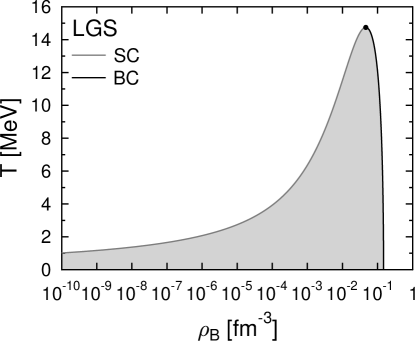
Figure 3: The binodal line which encloses the coexistence region (filled with gray) in the $T$ - $\rho_{B}$ plane for case LGS. The black dot marks the critical point (CP). The gray line to the left of the CP is the saturation curve (SC), and the black line to the right is the boiling curve (BC).

In Fig. 2 we show the pressure-temperature phase diagram, where we also obtain a phase transition line. Note that the pressure on the coexistence line goes to zero in the zero-temperature limit. For a congruent PT the Clapeyron-equation is valid:

$$\frac{dP}{dT}=\frac{s^{I}-s^{II}}{1/\rho_{B}^{I}-1/\rho_{B}^{II}}\;,$$ (35)

with $s^{I}=S^{I}/B^{I}$ and $s^{II}=S^{II}/B^{II}$ denoting the entropy per baryon of the two phases. The Clapeyron-equation describes how the slope of the pressure-temperature phase transition line is related to the difference in baryon number density and entropy per baryon of the two phases. In our investigation, we always have $\rho_{B}^{I}<\rho_{B}^{II}$, i.e. the first phase is assumed to have lower density. In Fig. 2 we see that $dP/dT>0$, and thus $s^{G}>s^{L}$ (where we have replaced “$I$” by “$G$” and “$II$” by “$L$”). The gas phase has a higher entropy per baryon and is always less dense than the liquid phase, which is a characteristic of the LGPT.

In Fig. 3 the binodal region is shown in the temperature-density plane. The gray line to the left of the critical point depicts the SC, where droplets of liquid form within the nucleon gas. The black line is the BC, where bubbles of gas form inside the liquid. The region enclosed by the two lines is the phase coexistence region, where a two-phase mixture of gas and liquid is present. Here, and also in all following plots, filled areas correspond to states of such a two-phase coexistence. Due to the congruent behavior of LGS, for each point inside the binodal or phase coexistence region, the gas state on the SC is in coexistence with the liquid state on the BC at the same common temperature. Thus the gas and the liquid are distinguished from each other by density, whereas the liquid is always more dense. At the critical point the two phases are identical. Inside the phase coexistence region, the volume fraction of the liquid phase $\alpha={V^{L}}/{V}$ and the gas phase ($1-\alpha$) are set by the total baryon number density $\rho_{B}=B/V$ through:

$$\rho_{B}=\rho_{B}^{G}(1-\alpha)+\rho_{B}^{L}\alpha\;.$$ (36)

Obviously, one has $\alpha=0$ on the SC and $\alpha=1$ on the BC.

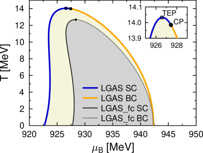
Figure 4: (Color online) Phase diagram in the temperature - baryon chemical potential plane for the two asymmetric systems LGAS and LGAS_fc with $Y_{Q}=0.3$. The gray and black thin lines show the forced-congruent variant LGAS_fc, and the corresponding small black dot is the pseudo-critical point. The colored thick lines depict case LGAS, where $Y_{Q}$ is not constrained locally. The corresponding black dot is the critical point and the open square the temperature endpoint. The inlay shows a zoom-in to the region around the critical point (CP) and temperature endpoint (TEP) of the non-congruent case LGAS. The filled areas are the coexistence regions.

For asymmetric nuclear matter in the case LGAS one obtains a non-congruent phase transition, which can be seen in Fig. 4, depicted by the orange and blue thick lines. For the non-trivial solution of the equilibrium conditions in the non-congruent case we have used the method described in Ref. Ducoin et al. (2006). The gray and black thin lines show the forced congruent variant LGAS_fc which will be discussed later. For LGAS one has a phase coexistence region in $T$-$\mu_{B}$, enclosed by the orange and blue thick lines, instead of a single line as in Fig. 1 for LGS. Also in all following plots, we will use colored thick lines for NCPTs. Thus one can also distinguish between the branch belonging to the SC and the branch belonging to the BC by different colors.

As it was stressed in Refs. Iosilevskiy (2010, 2011), in non-congruent VdW-like phase transitions of gas-liquid type there is no more a unique “critical endpoint”. Instead, three separate endpoints exist: maximal temperature (cricondentherm), maximal pressure (cricondenbar), and point of extremal chemical potential. In NCPT, these three “topological” endpoints are separated from the singular thermodynamic object—the true non-congruent critical point. Note also that the critical point of a congruent phase transition is determined by:

$$\left.\frac{\partial P}{\partial\rho_{B}}\right|_{T}=\left.\frac{\partial^{2}P}{\partial\rho_{B}^{2}}\right|_{T}=0\;.$$ (37)

In contrast, for a NCPT this criteria is not applicable, and the critical point does not fulfill it in general.

The inlay of Fig. 4 shows that the temperature endpoint is different from the critical point. For LGAS, the critical point is found at $T^{\rm CP}=13.99$ MeV (lower than in LGS) and $\mu_{B}^{\rm CP}=927.4$ MeV. It is very interesting that this reduction of the critical temperature agrees very well with the experimental results of Refs. McIntosh et al. (2013). The further properties of the critical point are given in Table 4. The temperature endpoint is located at $T^{\rm TEP}=14.03$ MeV and $\mu_{B}^{\rm TEP}=926.6$ MeV. We remark that for LGAS the temperature endpoint is located on the saturation curve (blue thick line), which in principle could also be located on the boiling curve (orange thick line). This topology (i.e., location of the temperature endpoint on the two-phase boundary relative to the critical point) is the same as for the gas-liquid NCPT in uranium-oxygen plasma Iosilevskiy et al. (2001, 1999, 1997, 1999); Ronchi et al. (2004); Iosilevskiy (2011); Iosilevskiy et al. (2003), which is taken as the prototype of NCPT for the present study of LGAS (compare Figs. 5 and 6 with Fig. 1 of Ref. Iosilevskiy (2010)).

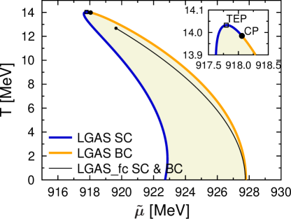
Figure 5: (Color online) Phase diagram in the plane of temperature and Gibbs free energy per baryon $\tilde{\mu}$ for case LGAS and LGAS_fc ($Y_{Q}=0.3$). Otherwise the same notation and depiction as in Fig. 4 is used.

In LGAS_fc the two phases are constrained locally to have the same charge fraction $Y_{Q}^{G}=Y_{Q}^{L}=0.3$. The results are depicted by the gray and black thin lines in Fig. 4. The two lines also enclose a phase coexistence region, which illustrates the non-equality of $\mu_{B}$ of the two phases in the phase coexistence region, due to the locally constrained charge fraction (see also the discussion in Sec. V.3 and Appendix C.1). The Gibbs free energy per baryon $\tilde{\mu}$ is the only chemical potential which is equal in the two phases. Furthermore, for isothermal phase transitions it is a constant, because the properties of the two phases do not change. In contrast to the non-congruent phase transition LGAS, for the forced-congruent phase transition LGAS_fc $\mu_{B}$ is dependent on the baryon number density $\rho_{B}$ and given by:

$$\mu_{B}=\mu_{B}^{G}\frac{\rho_{B}^{G}}{\rho_{B}}(1-\alpha)+\mu_{B}^{L}\frac{\rho_{B}^{L}}{\rho_{B}}\alpha\;,$$ (38)

which is derived in Appendix C.1.

The phase diagrams as a function of the Gibbs free energy per baryon $\tilde{\mu}$ are shown in Fig. 5 for both cases LGAS and LGAS_fc. The banana-shaped region of LGAS is typical for non-congruent liquid-gas like phase transitions, see Refs. Iosilevskiy et al. (2001, 1999, 1997, 1999); Ronchi et al. (2004); Iosilevskiy (2011); Iosilevskiy et al. (2003). In Fig. 5 the congruence of LGAS_fc becomes obvious. Comparing LGAS and LGAS_fc, the phase coexistence region turns into a phase coexistence line, when enforcing the local constraint for the charge fraction. Furthermore, for LGAS_fc the pseudo-critical point (properties listed in Table 4) coincides with the temperature and chemical potential endpoints. Note that the pseudo-critical point of a forced-congruent phase transition obeys Eq. (37). We remark that the phase transition line of the forced-congruent variant must lie strictly inside the two-phase region of the non-congruent phase transition Iosilevskiy et al. (2001, 1999, 1997, 1999); Ronchi et al. (2004); Iosilevskiy (2011); Iosilevskiy et al. (2003), which also can be seen as a consequence of Le Chatelier’s principle. As an exception, both objects could touch each other in azeotropic points of the parameter space, as seen for LGS.

Note that for the LGS case, $\mu_{B}=\tilde{\mu}$, since $\mu_{Q}\equiv 0$. Thus the phase-coexistence line of LGAS_fc in Fig. 5 can be directly compared with the one of LGS in Fig. 1 and it is found that their shape is very similar. However, states on the phase coexistence line of LGAS_fc in Fig. 5 belong to two different values of the baryon chemical potential, shown by the two gray and black thin lines in Fig. 4. If $\tilde{\mu}$ in LGAS_fc were changed in a continuous way and the phase transition line in Fig. 5 is crossed, $\mu_{B}$ jumps from the value of the gas phase to the value of the liquid phase in Fig. 4. This can be seen as a sign of the enforced congruence, in contrast to the azeotropic congruent phase transition LGS.

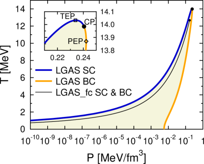
Figure 6: (Color online) Phase diagram in the plane of temperature and pressure for cases LGAS and LGAS_fc ($Y_{Q}=0.3$). In addition to the critical point (black dot), the temperature (open square) and pressure endpoints (open diamond) are shown in the inlay. Otherwise the same notation and depiction as in Fig. 4 is used.

Figure 6 shows the same scenarios as the previous figures, but gives the phase diagrams in the temperature-pressure plane. Here it is clear, that the phase transition in the forced congruent variant LGAS_fc occurs only at a single value of the pressure, which is the same behavior as in Fig. 2 for LGS. In contrast, for a given temperature in LGAS, there is an extended coexistence range in pressure, which is enclosed by the SC and BC. The names “SC” and “BC” are widely accepted for non-congruent evaporation in chemically reacting plasmas Iosilevskiy et al. (2001, 1999, 1997, 1999); Ronchi et al. (2004); Iosilevskiy (2011) where there meaning is obvious. They are also most intuitive for LGAS for this kind of phase diagram: for a fixed pressure of e.g. $10^{-2}$ MeV/fm³ and starting from $T=0$, by heating the system one will reach the boiling curve, where bubbles of gas appear inside the liquid. Conversely, if one starts at high temperatures and cools the system isobarically, droplets of liquid will form within the gas when the saturation curve is reached. In this figure we can also identify the pressure endpoint which is located on the BC of LGAS. In the gas-liquid NCPT in uranium-oxygen plasma Iosilevskiy et al. (2001, 1999, 1997, 1999); Ronchi et al. (2004); Iosilevskiy (2011); Iosilevskiy et al. (2003), which is the prototype for our present study of NCPT in LGAS, one has the same topology that the pressure endpoint is located on the BC, despite differences in the thermodynamic variables by many orders of magnitude (compare Fig. 6 with Fig. 1 in Ref. Iosilevskiy (2010)). For LGAS_fc, all three endpoints coincide with the critical point defined by Eq. (37) (see Fig. 1 in Ref. Iosilevskiy (2010)).

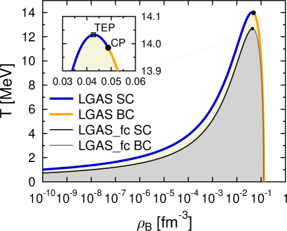
Figure 7: (Color online) The binodal line enclosing the coexistence region in the $T$ - $\rho_{B}$ plane for LGAS and LGAS_fc ($Y_{Q}=0.3$). Otherwise the same notation and depiction as in Fig. 4 is used.

In spite of the similarity of the NCPT in LGAS with its terrestrial prototypes Iosilevskiy et al. (2001, 1999, 1997, 1999); Ronchi et al. (2004); Iosilevskiy (2011); Iosilevskiy et al. (2003), the significant difference in the topology of P–T diagrams should be stressed (compare Fig. 6 above with Fig. 1 in Ref. Iosilevskiy (2010)). While the pressure on both boundaries of the non-congruent PT in the uranium-oxygen system Iosilevskiy et al. (2001, 1999, 1997, 1999); Ronchi et al. (2004); Iosilevskiy (2011); Iosilevskiy et al. (2003)—boiling and saturation curves—tends to zero for the limit $T\rightarrow 0$, the pressure on the boiling curve in NCPT in asymmetric ($Y_{Q}=0.3$) LGPT does not tend to zero when $T\rightarrow 0$ in our case (see Fig. 6). The same feature was noted already for the NCPT of asymmetric nuclear matter calculated with a different EOS (Fig. 3 in Ref. Maruyama and Tatsumi (2011)). The reason for this feature is the difference in the physical nature of the involved forces which are relevant for the non-congruence in a chemically-reacting uranium-oxygen plasma Iosilevskiy et al. (2001, 1999, 1997, 1999); Ronchi et al. (2004); Iosilevskiy (2011); Iosilevskiy et al. (2003) and in asymmetric nuclear matter, and also the use of Fermi-Dirac statistics for the latter.

In Fig. 7 we show the binodal or phase coexistence regions for LGAS and LGAS_fc in the temperature - density plane, similar as in Fig. 3 for LGS. Again, the non-congruent behavior of LGAS can be identified by the non-equivalence of the temperature endpoint and the critical point. Conversely, for LGAS_fc the endpoints and the (pseudo-) critical point coincide. Furthermore, for isothermal processes of LGAS at temperatures $T^{\rm CP}<T<T^{\rm TEP}$ so-called retrograde condensation occurs (see also Ref. Barranco and Buchler (1980); Müller and Serot (1995)): imagine, e.g., an isothermal compression at $T=14$ MeV. First one hits the saturation curve from the left, and a liquid with a larger $Y_{Q}$ and a larger $\rho_{B}$ appears inside the gas phase. With increasing density the volume fraction of the liquid will first increase. But for retrograde condensation, for densities larger than a certain density, the volume fraction will decrease again, until it returns to zero at the right side of the saturation curve. The liquid has disappeared again after the phase coexistence region has been crossed.

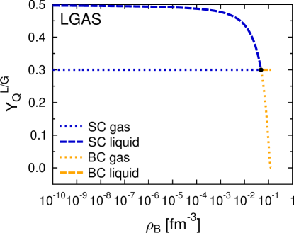
Figure 8: (Color online) The charge fraction of the liquid (dashed lines) and the gas phase (dotted lines) for case LGAS as a function of the coexistence density $\rho_{B}$ along the binodal line of Fig. 7. The blue lines show the charge fractions of the two coexisting phases for states on the saturation curve presented in previous figures, the orange lines for states on the boiling curve.

The non-congruent behavior of LGAS is further analyzed in the following plots of local “chemical” composition and density. Fig. 8 shows the charge fractions of the two phases which are in coexistence, if one moves along the liquid and vapor binodal lines of Fig. 7. The blue dotted line “SC gas” in Fig. 8 depicts the charge fraction of the gas phase $Y_{Q}^{G}$ for the states on the saturation curve shown in Fig. 7. On the saturation curve, the gas phase is in coexistence with a liquid phase which has a different charge fraction $Y_{Q}^{L}$, shown by the dashed blue line. Also for the conditions of the boiling curve of Fig. 7, we always have coexistence of a gas phase (orange dotted line in Fig. 8) with a liquid phase (orange dashed line in Fig. 8), which have different charge fractions.

In all previous plots, the depicted quantities correspond to total thermodynamic quantities, i.e. of the system as a whole. In contrast, in Figs. 8, 9, and 10 we are showing individual properties of the two coexisting phases. Now and in the following we are using dashed and dotted lines in such plots to illustrate this difference. The color coding helps to identify the same states in the different diagrams. For example in Fig. 8, the ends of the orange curves, which correspond to $T=0$, are given by the highest density of coexistence of LGAS in Fig. 7 which is on the orange solid line.

In Fig. 8, one of the two phases always must have $Y_{Q}=0.3$, whereas the charge fraction of the second phase is not constrained, because its volume fraction is still zero on the binodal line. For states on the saturation curve one is still in the gas phase, i.e. $\alpha=0$, thus $Y_{Q}^{G}=0.3$. For states on the boiling curve one is still in the liquid phase, $\alpha=1$, and $Y_{Q}^{L}=0.3$. The charge fraction is an order parameter for LGAS and thus it can be used to characterize the two phases, with the identification that the gas phase always has a lower charge fraction than the liquid, i.e. $Y_{Q}^{G}<Y_{Q}^{L}$. Only at the critical point is equality established, $Y_{Q}^{G}=Y_{Q}^{L}$. It is interesting to note, that the charge fraction of the phase with $Y_{Q}\neq 0.3$ shows the same dependence on density before and after the critical point.

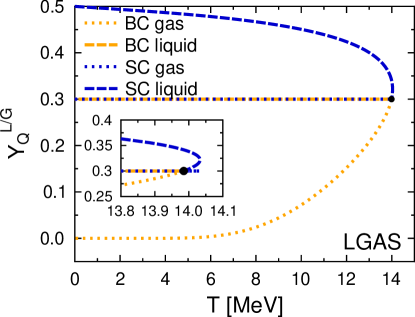
Figure 9: (Color online) As Fig. 8, but now in dependence of the coexistence temperature of the binodal line of Fig. 7. The inlay shows a zoom-in to the region around the critical point, including the region of so-called retrograde condensation at $T>T^{\rm CP}$.

In Fig. 9 we also show the charge fractions of the two phases along the binodal line, but now as a function of the coexistence temperature. By comparing with Figs. 4 - 7, it is obvious, that for each coexistence temperature there are always two points on the binodal line, corresponding to two different halves of the binodal line which are separated from each other by the temperature endpoint. For each half, two phases with different values of $Y_{Q}$ are in coexistence. Consequently, in Fig. 9, for each temperature there are always four values of $Y_{Q}$. For $T<T^{\rm CP}$, one has $Y_{Q}^{G}=0.3$ and $Y_{Q}^{L}>0.3$ on the saturation curve, and $Y_{Q}^{G}<0.3$ and $Y_{Q}^{L}=0.3$ on the boiling curve. Note that the two lines with $Y_{Q}=0.3$ are on top of each other. For $T^{\rm CP}<T<T^{\rm TEP}$, both halves belong to the saturation curve, and thus $Y_{Q}^{G}=0.3$ for both halves, each being in coexistence with a different configuration of the liquid with $Y_{Q}^{L}>0.3$.

The previous two figures can be used to identify the high degree of isospin distillation of LGAS in the limit $T\rightarrow 0$. Let us consider a decompression at $T\sim 0$ of the asymmetric system with $Y_{Q}=0.3$. Once the boiling curve is reached vapor bubbles appear which in this case consist of pure neutron gas, $Y_{Q}^{G}\rightarrow 0$. Obviously, this leads to the distillation of a symmetric liquid by evaporation of pure neutron bubbles from a boiling asymmetric liquid phase. On the other hand, for saturation conditions (“dewpoint”) at $T\sim 0$, liquid microdrops tend to the exactly symmetric composition, $Y_{Q}^{L}\rightarrow 0.5$. These features of the NCPT of case LGAS differ significantly from the behavior of the chemical composition (O/U-ratio) in NCPTs of uranium-oxygen systems (compare Fig. 9 with Fig. 2 of Ref. Iosilevskiy et al. (2001) and Fig. 3 of Ref. Iosilevskiy et al. (1999)).

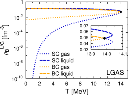
Figure 10: (Color online) The baryon number density of the liquid (dashed lines) and the gas phase (dotted lines) for case LGAS as a function of the coexistence temperature on the binodal line of Fig. 7. Otherwise the same notation and depiction as in Fig. 9 is used.

In a similar way as in Fig. 9, in Fig. 10 we show the baryon number densities of the two phases for each of the two halves of the binodal line as a function of the coexistence temperature. Presented in this way, one sees that the density is also an order parameter of LGAS, whereas the liquid is the phase with the higher density. At the critical point, the liquid and the gas have the same density and charge fraction and thus cannot be distinguished from each other any longer. The discussion of this figure is similar as for Fig. 9: For $T<T^{\rm CP}$ there are the $\rho_{B}$-curves from the liquid (blue dashed line) and the gas (blue dotted line) on the saturation curve, and another pair of $\rho_{B}$-curves from the liquid (orange dashed line) and the gas (orange dotted line) on the boiling curve. For $T^{\rm CP}<T<T^{\rm TEP}$ there are still the four different values of $\rho_{B}$. However, now all points belong to the saturation curve.

VI.2 Deconfinement phase transition

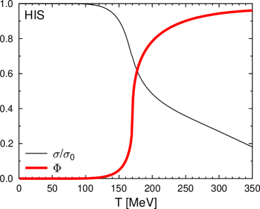
Figure 11: (Color online) Order parameter for chiral symmetry restoration/breaking $\sigma$ normalized by the vacuum value $\sigma_{0}$ and order parameter for deconfinement/confinement $\Phi$ versus temperature at zero baryon chemical potential for symmetric matter of case HIS ($Y_{Q}=0.5$).

For the LGPT we used the baryon number density and charge fraction as order parameters. For the deconfinement and chiral symmetry PTs, typically the Polyakov-loop $\Phi$ and the chiral condensate $\sigma$ are used, as already discussed in Sec. IV. The field $\sigma$ characterizes chiral symmetry restoration whereas $\Phi$ can be taken as a measure for deconfinement. At finite temperature and $\mu_{B}=0$, respectively $\rho_{B}=0$, there is no first-order PT, but a smooth crossover between the hadronic (confined, chiral symmetry broken) and the quark phase (deconfined, chiral symmetry partly restored) Aoki et al. (2006). This is shown in Fig. 11 for HIS, where the ratio $\sigma/\sigma_{0}$ decreases from one to lower values and $\Phi$ goes from zero to a value close to one in a smooth fashion. We remark that we define the cross-over temperature $T^{\rm co}$ as the peak of the change of the chiral condensate and $\Phi$ with $T$, yielding a value of $T^{\rm co}=171$ MeV, in accordance with lattice QCD results Fodor and Katz (2004). This behavior of the order parameters corresponds to the example trajectory through the phase diagram of HIS shown in Fig. 12.

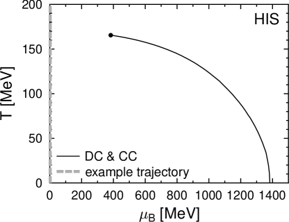
Figure 12: Phase diagram in the temperature - baryon chemical potential plane for case HIS ($Y_{Q}=0.5$), for which the deconfinement curve (DC) coincides with the confinement curve (CC). The black dot marks the critical point. The thick gray line along the y-axis shows part of the example trajectory belonging to Fig. 11.

For high enough baryon number densities, the QHPT turns into a first-order phase transition. This can be seen in Fig. 12 where we show the first-order phase transition line for case HIS, i.e. for heavy-ion collisions of symmetric nuclei. The critical point is located at $T^{\rm CP}=165.5$ MeV and $\mu_{B}^{\rm CP}=383$ MeV, again, in accordance with lattice QCD results Fodor and Katz (2004). Its further properties are listed in Table 4. The topology of this PT is the same as in LGS, see Fig. 1, only the typical scales are different. For example, the critical point of HIS is at a roughly ten times higher temperature. For the QHPT, we will use the terms “deconfinement curve” (DC) instead of “saturation curve” and “confinement curve” (CC) instead of “boiling curve”, which we think is more meaningful. If coming from low densities and temperatures, first droplets of denser deconfined quark matter will appear when the DC is reached. Conversely, if coming from high densities and temperatures, when the CC is reached, the first quarks will start to be confined into bubbles of less dense hadronic matter. There is an interesting analogy to the “ionization boundary curve” and “recombination boundary curve” of the hypothetical ionization-driven plasma phase transition in dense hydrogen at megabar pressure range (see, e.g., Fortov et al. (2006); Fortov (2011); Iosilevskiy and Starostin (2000)). This first-order PT in weakly ionized hydrogen (predominantly H and H₂ and small amount of p and e) is driven by a jump-like ionization (deconfinment) into highly ionized hydrogen (predominantly p and e and small amount of H and H₂). We want to point out the similarity between the hydrogen plasma which is an arbitrary solution of H₂, H, p, and e, and the Chiral SU(3) model in which quarks and hadrons can in principle also be mixed in arbitrary proportions (nevertheless a clear distinction of the two phases is always possible, see Sec. IV).

HIS is, in principle, a binary system, with baryon number and electric charge (respectively isospin) as two globally conserved charges (see Table 3). But the PT in HIS is azeotropic, meaning it is congruent and the Maxwell construction can be used, just like symmetric nucleonic matter in LGS. It is not so obvious as for LGS that matter in HIS is an azeotrope, because a whole set of particles, including strange ones, is considered (see Table 3). However, strange quarks and hyperons do not invalidate the relation between isospin symmetry and azeotropic behavior, if strangeness is set locally to zero, as it is done here. In this case, the total density of strange quarks, i.e. in form of unbound strange quarks or bound in hyperons, is equal to the total density of anti-strange quarks. A more detailed explanation of the matter is given in Appendix B.

Figure 13: Phase diagram in the temperature - pressure plane for case HIS. Otherwise notation and depiction as in Fig. 12.

In Fig. 13 the phase diagram in the pressure-temperature plane is depicted. Comparing with Fig. 2 one realizes an important difference between the QHPT and the LGPT: the slope of the phase transition line is negative. Therefore, the QHPT is not of liquid-gas type. With the Clapeyron equation (35) one finds that this is due to the fact that the hadronic phase, which is less dense, has a lower entropy per baryon than the quark phase, $s^{H}<s^{Q}$ (where we have replaced “$I$” by “$H$” and “$II$” by “$Q$”), which is opposite to the behavior in the LGPT. The negative slope of the $p-T$ phase diagram makes the QHPT fundamentally different from the LGPT. This fact (negative slope of the $p-T$ boundary for QHPT in a symmetric system) is not absolutely new (e.g., presentations of I.I. at several conferences and discussion in Ref. Iosilevskiy and Starostin (2000), L. Satarov, private communication (2010) based on calculations via EOS model described in Satarov et al. (2009), J. Randrup, presentations at several conferences and Ref. Randrup (2012), or Yudin et al. (2013)) but is not well-recognized yet. Further investigation and analysis of this fundamental difference between LGPT and QHPT is in preparation Iosilevskiy and Randrup (2013). Fig. 14 shows the coexistence region in the temperature - baryon number density plane, in a similar way to Fig. 3 for the LGPT. Note that the shape of the phase coexistence region of HIS is rather different from LGS. This is once more a manifestation (and not the last one) of the fundamental difference between LGPT and QHPT.

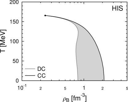
Figure 14: Phase diagram in the temperature - baryon number density plane for case HIS. The deconfinement curve (DC) is to the left of the confinement curve (CC). The gray area shows the two-phase coexistience region. Otherwise notation and depiction as in Fig. 12.

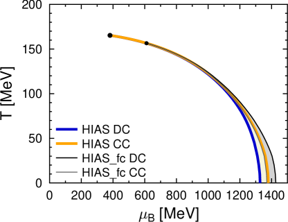
Figure 15: (Color online) Phase diagram in the temperature - baryon chemical potential plane for cases HIAS and HIAS_fc ($Y_{Q}=0.3$). The colored thick lines belong to HIAS, the gray and black thin ones to HIAS_fc. The large black dot marks the critical point of HIAS and the small black dot the pseudo-critical point of HIAS_fc. The filled areas show the coexistence regions. Note that for HIAS_fc the confinement curve (CC) is to the left of the deconfinement curve (DC).

In case HIAS of heavy ion collisions with asymmetric Coulomb-less matter one has a true binary system. The PT is non-congruent and the Gibbs construction must be used. This is visible in Fig. 15, where one obtains a phase-coexistence region instead of a phase-transition line as in HIS before. We can compare HIAS with LGAS of Fig. 4. Obviously, the phase-coexistence region is much narrower than for LGAS, if we compare the width in $\mu_{B}$ relative to the extension in temperature. HIAS_fc is the forced congruent variant, where the charge fraction is constrained locally, $Y_{Q}^{H}=Y_{Q}^{Q}=0.3$, so that the Maxwell construction can be used. The gray thin line is the corresponding DC, and the black thin line the CC, which is partly covering the CC of HIAS. Very interestingly, the DC and CC changed order for HIAS_fc compared to HIAS. We will explain this interesting result in detail later.

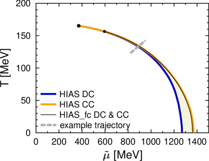
Figure 16: (Color online) Phase diagram in the plane of temperature and Gibbs free energy per baryon $\tilde{\mu}$ for cases HIAS and HIAS_fc ($Y_{Q}=0.3$). The thick gray line gives an example for a trajectory through the phase diagram for which we show the order parameters in Fig. 21. Otherwise the same depiction and notation as in Fig. 15 is used. Note that the phase transition line of HIAS_fc is very close to the confinement curve (CC) of HIAS.

The phase diagrams as a function of the Gibbs free energy per baryon $\tilde{\mu}$ are shown in Fig. 16, and as a function of pressure in Fig. 17. Here one sees that HIAS_fc is a congruent PT, because the DC and CC are identical. Furthermore, the phase transition line of HIAS_fc is inside the phase coexistence region of HIAS, as it has to be. Comparing Fig. 16 with Fig. 5 of LGAS, again one sees that the shape of the coexistence region of HIAS is much narrower. This could be described as a weaker non-congruence of the phase transition HIAS.

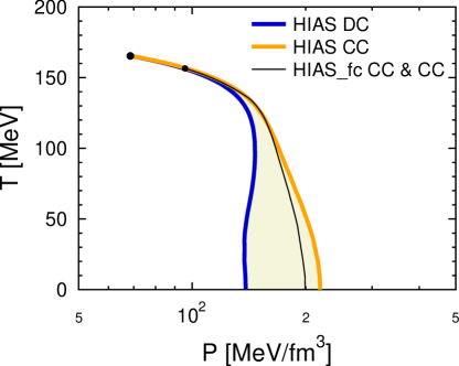
Figure 17: (Color online) Phase diagram in the temperature - pressure plane for HIAS and HIAS_fc ($Y_{Q}=0.3$). The same depiction as in Fig. 15 is used.

Note that in our calculations for HIAS we could not resolve the differences between the temperature and pressure endpoints and the critical point. In principle, around the critical point a similar structure as for LGAS has to occur. We predict that the phase coexistence regions of HIAS around the critical point are smooth and two-dimensional, like for LGAS in the inlays of Figs. 4-7, whereas the temperature endpoint and critical point could also have their orders inversed. To be more precise, we expect a round, “banana-shaped” region (see, e.g., Fig. 1 in Iosilevskiy (2010)). However, due to the fact that for lower chemical potentials or baryon densities the first-order phase transitions HIS and HIAS become rather weak, i.e., the phases on both sides of the transition become extremely similar, this structure is not as easily observed anymore as it is in the LGPT of nuclear matter (shown in the previous subsection) and in chemically reacting plasmas Iosilevskiy et al. (2001, 1999, 1997, 1999); Ronchi et al. (2004); Iosilevskiy (2011); Iosilevskiy et al. (2003). The highest temperature, for which we still could solve the equilibrium conditions was at $T=165.3$ MeV for $\mu_{B}=381$ MeV, respectively $\tilde{\mu}=371$ MeV where we used a resolution of roughly $0.1$ MeV in temperature. Because this resolution cannot be resolved on the scale of Fig. 15, we take these values of $T$, $\mu_{B}$, and $\tilde{\mu}$ as the approximate temperature and chemical potentials of the critical point, which are also listed in Table 4. The very narrow phase coexistence region shows that the two phases are in an extremely similar thermodynamic state. For even higher temperatures, the differences between the two phases become smaller than our numerical accuracy, preventing us to find a more precise solution.

This aspect is also very pronounced in Fig. 18 where the phase diagrams of HIAS and HIAS_fc are shown as a function of baryon number density. At $T=0$, the DC and the CC have very different densities. Conversely, for increasing temperatures the extension of the coexistence region in density becomes extremely narrow. Note that the coexistence region of HIAS_fc is within HIAS, as it must be.

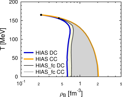
Figure 18: (Color online) Phase diagram in the plane of temperature and baryon number density for cases HIAS and HIAS_fc ($Y_{Q}=0.3$). Otherwise the same depiction and notation as in Fig. 15 is used. The deconfinement curve (DC) of HIAS_fc is now to the left of the confinement curve (CC).

There is one further important aspect. If we compare the phase diagram of the asymmetric system, e.g. Fig. 15, with the symmetric system in Fig. 12, and the corresponding numbers in Table 4, one finds that the critical points are practically unaffected by the change of the asymmetry. $T$ and $\mu_{B}$ of HIS and HIAS differ by less than 0.5 %. In LGPT, a stronger dependence on the asymmetry is observed. For LGS and LGAS the change from $Y_{Q}=0.5$ to $Y_{Q}=0.3$ leads to a significant shift of the critical point, e.g. on the order of 6 % in temperature. This is naturally explained by the high temperatures of order 160 MeV around the critical point of HI. The effect of the asymmetry becomes extremely weak, because the EOS in this regime is dominated by thermal contributions. Obviously, for $\mu_{B}\longrightarrow 0$ the EOS would be completely independent of the asymmetry. We conclude that even though HIAS is in principle a non-congruent PT, in our calculations with the Chiral SU(3) EOS model this non-congruence is almost negligible close to the critical point. This is also visible in Figs. 15 and 16, where the width of the coexistence region is smaller than the line thickness of the curves.

Let us now come back to the explanation of the inverted ordering of DC and CC in HIAS_fc in Fig. 15. For an isothermal compression, corresponding to a horizontal line through Fig. 18, $\tilde{\mu}$ and $\mu_{B}$ will increase monotonically, until the deconfinement curve is reached at a certain density $\rho_{B}=\rho_{B}^{H}$. This state corresponds to the value of $\mu_{B}=\mu_{B}^{H}$ in the hadronic phase on the deconfinement curve, i.e. the black thin line most to the right in Fig. 15. For an isothermal compression, the corresponding value of $\tilde{\mu}$ will remain constant throughout the phase transformation, and $\tilde{\mu}=\tilde{\mu}^{H}=\tilde{\mu}^{Q}$. However, inside the coexistence region $\mu_{B}$ will change with density because it is given by:

$$\mu_{B}=\mu_{B}^{H}\frac{\rho_{B}^{H}}{\rho_{B}}(1-\alpha)+\mu_{B}^{Q}\frac{\rho_{B}^{Q}}{\rho_{B}}\alpha\;,$$ (39)

with the volume fraction of the quark phase $\alpha$ (see Appendix C.1). For HIAS_fc, the hadronic phase has a higher baryon chemical potential than the quark phase, $\mu_{B}^{H}>\mu_{B}^{Q}$. Therefore an increase of the baryon number density inside the phase coexistence region will lead to a decrease of $\mu_{B}$. For $\alpha=1$, i.e. $\rho_{B}=\rho_{B}^{Q}$, the CC in Fig. 15 is reached. For even higher densities $\mu_{B}$ will increase again.

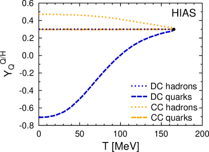
Figure 19: (Color online) The charge fractions of the hadronic ($Y_{Q}^{H}$, dotted lines) and the quark phase ($Y_{Q}^{Q}$, dashed lines) as a function of the coexistence temperature along the phase boundary, for case HIAS. The blue lines show states on the deconfinement curve DC, and the orange on the confinement curve CC.

Figures 19 and 20 show the charge fraction of each phase (hadronic and quark) as a function of the temperature and the baryon density along the phase boundaries. For clarity, we again distinguish states on the deconfinement curve by blue color and states on the confinement curve by orange. In Figures 19 and 20 one sees that the charge fraction in the quark phase is always less than or equal to the charge fraction in the hadronic phase. This shows that the charge fraction is also an order parameter of the QHPT. Note that $Y_{Q}^{Q}\leq Y_{Q}^{H}$ is the opposite behavior compared to the liquid-gas PT, in which the denser phase is more symmetric.

Note also that $Y_{Q}$ can in principle take negative values for both the hadronic and the quark phase, due to negatively charged hyperons, respectively down and strange quarks. In the LGPT we only considered neutrons and protons, so that $0\leq Y_{Q}\leq 1$. For HIAS we have $-1\leq Y_{Q}\leq 1$. Indeed we observe in Fig. 19 that $Y_{Q}^{Q}<0$ on the DC for coexistence temperatures below approximately 100 MeV. This means that the first quark matter droplets which would appear at the deconfinement phase boundary of the hadronic phase (DC) are negatively charged for such temperatures. Remember that on the DC only $Y_{Q}^{H}$ is constrained to the value 0.3, and $Y_{Q}^{Q}$ is set by the equilibrium conditions. Conversely, if the PT is crossed coming from the high density side we have $Y_{Q}^{Q}=0.3$ on the CC. The hadronic phase on the CC shows the opposite tendency than quark matter. For low temperatures it approaches a rather symmetric configuration with $Y_{Q}$ close to 0.5. Similar features have been discussed, e.g., in Ref. Fischer et al. (2011) for a simple quark-bag model. Fig. 20 appears quite complex and looks different to the equivalent Fig. 8 of LGAS. This can be explained by the non-monotonous behavior of the density as a function of the coexistence temperature in case HIAS, visible in Fig. 18.

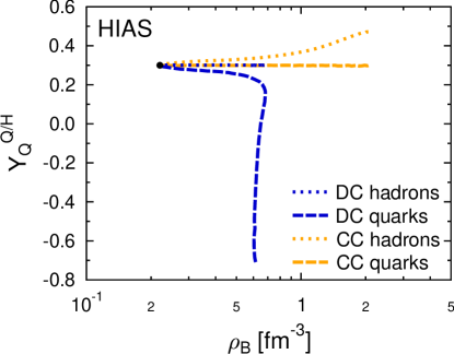
Figure 20: (Color online) As Fig. 19, but as a function of the coexistence baryon density.

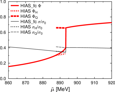
Figure 21: (Color online) Normalized order parameter for chiral symmetry restoration/breaking $\sigma$ (black thin lines) and order parameter for deconfinement/confinement $\Phi$ (red thick lines) versus the Gibbs free energy per baryon $\tilde{\mu}$ for case HIAS. Inside the phase coexistence region, the values of the order parameters in the quark phase (dashed lines) are different from the ones in the hadronic phase (dotted), and change during the phase transformation. HIAS_fc is the forced congruent variant, shown by solid lines. All order parameters are calculated for the trajectory through the phase diagrams shown in Fig. 16 with $T=0.15\tilde{\mu}$.

The two figures 19 and 20 also show how the charge fraction in both phases goes to $0.3$ when approaching the critical point. At the critical point, the two phases are identical, i.e. have the same charge fraction, density, scalar field $\Phi$, chiral condensate, etc. To better understand the dynamics of such a NCPT, in Fig. 16 we included an example for a trajectory through the phase diagram for which we show the order parameters in Fig. 21. The trajectory was chosen to follow $T=0.15\tilde{\mu}$ so that the phase coexistence region is crossed at temperatures around 900 MeV and $\tilde{\mu}\sim 130$ MeV. This trajectory could e.g. be realized during the decompression of the quark-gluon plasma in a heavy-ion collision. We show the behavior of the order parameters for HIAS and HIAS_fc to illustrate the differences between a non-congruent and congruent PT. For HIAS_fc, when the phase transition line is crossed, there are jumps in $\sigma$ and $\Phi$, as expected for a first-order PT (compare also with Fig. 11). The quark phase is characterized by having a larger value of $\Phi$, showing that it represents the deconfined state. As can be seen from Eqs. (5) and (6), this increases the effective mass of baryons, but decreases the effective mass of quarks. Note that $\sigma$, which is decreasing with increasing $\tilde{\mu}$ in both of the two phases, locally increases at the PT (going from left to the right), because the value of $\sigma$ is higher in the quark phase. This is in contrast to the typical expectation of other models which give partial chiral symmetry restoration, i.e., a lower value of $\sigma$ in the quark phase. This effect found in our calculations comes from the fact that in the Chiral SU(3) model both order parameters $\sigma$ and $\Phi$ are connected through the effective masses of the particles. Also the baryonic density of the quarks (not counting the contribution from $U$) is less than the one of the hadrons. This leads to a decrease of the scalar field across the phase transition.

In Fig. 21 it can be seen that in the non-congruent phase transition HIAS the behavior of the order parameters is more complex. Within the phase coexistence region, i.e. within the DC and CC shown in Fig. 16, the hadronic and the quark phases are in coexistence. The two phases are spatially separated and in each of the two phases one has different values of the order parameters. At the onset of the PT at the confinement curve one has $\alpha=1$, i.e. the volume fraction of the quark phase is still one and the volume fraction of the hadronic phase is 0. Inside the phase coexistence region, the quark phase has a larger value of $\Phi$, but also a slightly increased chiral condensate $\sigma$, as observed for HIAS_fc before. With decreasing $\tilde{\mu}$, not only the volume fraction of the quark phase decreases, but also the properties of the two phases change. One clearly sees that chiral symmetry breaking proceeds in both of the two phases with decreasing density. On the other hand $\Phi^{H}$ is decreasing, and $\Phi^{Q}$ is slightly increasing. When the deconfinement curve is reached, $\alpha=0$ and only the hadronic phase is left. After this in Fig. 21 one sees that $\Phi^{H}$ and $\sigma^{H}$ become equal to values obtained for HIAS_fc.

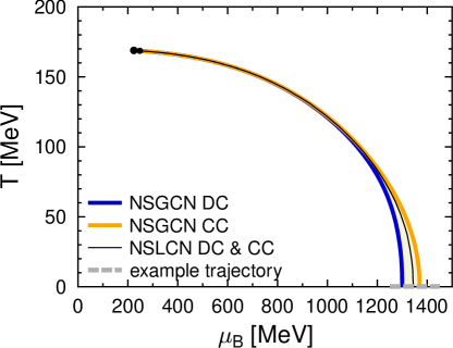
Figure 22: (Color online) Phase diagram in the temperature - baryon chemical potential plane for neutron stars with local (NSLCN) and global charge neutrality (NSGCN). The horizontal thick gray line at $T=0$ is a trajectory through the phase diagram, for which we show the order parameters in Fig. 23. The large black dot is the critical point of NSGCN, the small one the pseudo-critical point of NSLCN.

Finally, we discuss results for the quark-hadron phase transition in neutron stars shown in Fig. 22. Let us reiterate that in this paper we consider the quark-hadron PT in multi-component matter of neutron stars of macroscopic coexisting phases (i) with local charge neutrality and (ii) in the variant of global charge neutrality within the Coulomb-less approximation. It is just the Coulomb-less approximation which justifies the use of Gibbs conditions instead of Gibbs-Guggenheim conditions, which are valid for true macroscopic Coulomb systems (e.g., Ref. Iosilevskiy (2010)). Local and global charge neutrality constraints lead to forced-congruent (“Maxwell”) and non-congruent (“Gibbs”) PTs. As discussed in Sec. II.2, the choice between local or global charge neutrality can be associated with the unknown surface tension between the two phases.

The phase diagram of neutron stars looks similar to the one shown in Fig. 16. In contrast, the dimensionality of HIAS_fc in Fig. 15 is different to the one of NSLCN in Fig. 22. This is easy to understand, because $\mu_{B}^{Q}=\mu_{B}^{H}$ is valid for NSLCN and NSGCN, and also for HIAS, but not for HIAS_fc. The critical points of the neutron star cases are at lower $\mu_{B}$ and slightly higher $T$ than in cases HIAS and HIS, i.e., the phase transition regions extend to higher temperatures. Asymmetry and charge neutrality do not seem to have a major effect at such high temperatures. Therefore we relate this difference to the treatment of strangeness (see Table 3). At $T=0$ the width of the phase coexistence region of HIAS is 52 MeV, for NSGCN it is 70.2 MeV. With the chiral SU(3) model used here, the hadron-quark PT and the non-congruent features at $T=0$ seem to be stronger for neutron star matter than for matter in heavy-ion collisions. This is a result of the larger asymmetries obtained in beta-equilibrium due to the large degeneracy of electrons, and also because of the different constraints used for strangeness.

The critical point of NSGCN is at approximately $T^{\rm CP}=168.9$ MeV and $\mu_{B}^{\rm CP}=224$ MeV, the one of NSLCN at $T^{\rm CP}=168.6$ MeV and $\mu_{B}^{\rm CP}=247$ MeV (see also Table 4). Interestingly, they are only slightly different. It shows that the treatment of electric charge neutrality plays only a minor role for the location of critical points of the QHPT at the typical high temperatures. The local constraint applied in HIAS_fc which does not allow isospin diffusion, has a slightly larger effect at high temperatures.

The phase transition line for NSLCN with enforced local charge neutrality must lie strictly within the phase coexistence region of NSGCN, in accordance with general rules for NCPTs (e.g., Refs. Iosilevskiy et al. (2001, 1999, 1997, 1999); Ronchi et al. (2004); Iosilevskiy (2011); Iosilevskiy et al. (2003)). Both boundaries can touch each other in points of azeotropic composition. Here this would mean that the two phases were charge neutral a priori. Actually this is not the case, but they only touch because of the thickness of the lines in the figure. For NSLCN, $\mu_{Q}$ will not behave continuously when the phase transition line is crossed, as already discussed at the end of Sec. V.3, because $\mu_{Q}^{H}$ is different from $\mu_{Q}^{Q}$. This is in accordance with general properties of phase coexistence of charge neutral, macroscopic phases in Coulomb systems (see, e.g., Refs. Iosilevskiy (2010, 2011); Iosilevskiy, I. and Chigvintsev, A. (2000) and Aqua et al. (2005)): any phase-interface in macroscopic equilibrium Coulomb systems is accompanied by a finite difference in the average electrostatic potentials of both coexisting phases (Galvani potential), see also Sec. II.2 and compare also with Ref. Mishustin et al. (2010). However, the total charge chemical potential $\mu_{Q}$ still can be related to the local chemical potentials $\mu_{Q}^{H}$ and $\mu_{Q}^{Q}$, if it is seen as a function of baryon number density. Based on two different assumptions about the implementation of local charge neutrality, in Appendix C.3 we derive the following expressions:

$$\mu_{Q}=\begin{cases}(1-\alpha)\mu_{Q}^{H}+\alpha\mu_{Q}^{Q},&\mbox{for }\rho_{Q}^{H}\equiv\rho_{Q}^{Q}\\ (1-\alpha)\frac{\rho_{B}^{H}}{\rho_{B}}\mu_{Q}^{H}+\alpha\frac{\rho_{B}^{Q}}{\rho_{B}}\mu_{Q}^{Q},&\mbox{for }Y_{Q}^{H}\equiv Y_{Q}^{Q}\end{cases}$$ (40)

It would be more intuitive to assume the first of the two conditions. These expressions can be used to determine the total chemical potential of charged particles inside the two-phase mixture.

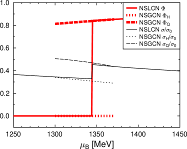
Figure 23: (Color online) As Fig. 21, but now for cases NSLCN and NSGCN of the example trajectory at $T=0$.

Fig. 22 also includes an example trajectory through the phase transition region at $T=0$. This trajectory could correspond e.g. to the spatial structure inside a neutron star, or better called hybrid star. In Fig. 23 we show the behavior of the order parameters for cases NSLCN and NSGCN along the trajectory. For $T=0$, we find $\Phi^{H}=0$, i.e. the hadronic phase is completely confined. For finite temperature this is different as can be seen in Figs. 11 and 21, where one has some sequential deconfinement already in the hadronic phase. Otherwise similar features are observed as in Fig. 21. The obtained jumps show that we have a first-order PT. The different values of the order parameters distinguish the two spatially separated phases. If the PT is non-congruent, one obtains a phase coexistence region, and the phases change their properties, including the order parameters, during the phase transformation.

VII Summary and Conclusions

In this article we investigated the liquid-gas phase transition (LGPT) described by the FSUgold relativistic mean-field model and the hadron-quark (HQ) or deconfinement phase transition with the Chiral SU(3) model. We did not take into account any explicit Coulomb interactions or other finite-size effects, but always considered phase coexistence of macroscopic phases. Different physical systems were investigated: heavy ion collisions of symmetric nuclei at low (LGS) and high collision energies (HIS) and of asymmetric nuclei with $Z/A=0.3$ at low (LGAS) and high collision energies (HIAS). Furthermore, we also studied the QHPT in neutron stars (NS). The main goal of our work is to characterize the first-order phase transitions in the different systems regarding their possible non-congruence and to identify the typical non-congruent aspects. This characterization and classification, and our qualitative results should not depend on the model used for the calculations, but should be valid in a rather general way. In our study of non-congruent phase transitions we used essential features of such type of phase transitions obtained from terrestrial applications with high-temperature chemically reacting plasmas Iosilevskiy et al. (2001, 1999, 1997, 1999); Ronchi et al. (2004); Iosilevskiy (2011); Iosilevskiy et al. (2003).

Table 4: Approximate location of the critical and pseudo-critical points of the different scenarios.

case	$T$ [MeV]	$\rho_{B}$ [fm-3]	$\mu_{B}$ [MeV]	$p$ [MeV/fm3]
LGS	14.75	0.046	912.4	0.205
LGAS	13.99	0.049	927.4	0.241
LGAS_fc	12.68	0.044	928.3	0.171
HIS	165.5	0.24	383	73.1
HIAS	165.3	0.22	381	68.6
HIAS_fc	156.5	0.44	611	95.8
NSLCN	168.6	0.16	247	162.8
NSGCN	168.9	0.14	224	161.1

A non-congruent, first-order phase transition occurs for a non-unary system with more than one (globally) conserved charge where the charge ratios change during a phase transformation. In principle, all the investigated scenarios contain several conserved charges, with at least baryon number and electric charge. However, due to isospin symmetry, for the symmetric case (LGS and HIS), matter always stays symmetric, even if there is phase-coexistence, which is called “azeotropic” behavior. Only these two cases lead to congruent phase transitions. To further illustrate the differences between a congruent and a non-congruent phase transition, we also considered the cases LGAS_fc and HIAS_fc, where we forced the system to have a congruent phase transition, by constraining the local charge fractions to be equal in the two phases. From a physical point of view the forced-congruent regime of phase transformations is not completely artificial, but corresponds to the so-called “frozen diffusion approximation”. In a similar way we considered enforced local charge neutrality in neutron stars in case NSLCN instead of global charge neutrality NSGCN. In Table 5 we summarize the classification of the phase transitions in the different physical systems.

In the astrophysics community, congruent and non-congruent phase transitions are usually called “Maxwell” and “Gibbs” phase transitions, referring to the way in which phase coexistence is calculated. Because of the constant charge ratios and the fact that all properties of the two phases do not change for an isothermal phase transformation, a simple Maxwell construction can be used for the congruent case. Conversely, for non-congruent phase transitions the more complicated Gibbs construction is necessary to solve the set of thermal, mechanical and multiple chemical equilibrium conditions. Due to their prominent role in neutron star physics, NSLCN and NSGCN are considered as the two most representative scenarios. However, as we demonstrated, they are only examples illustrating the further classification of first-order phase transitions to be either congruent or non-congruent.

The distinction between congruent and non-congruent phase transitions is crucial for the dimensionality of phase diagrams. For a given temperature $T$, a congruent phase transition occurs at a single value of the Gibbs free energy per baryon $\tilde{\mu}$. Therefore in the $T$-$\tilde{\mu}$-plane, one obtains a phase transition line, as well as in the $T$-$P$- and $P$-$\tilde{\mu}$-planes, and generally in any pair of intensive thermodynamic variables Iosilevskiy (2010). Conversely, for a non-congruent phase transition calculated with the Gibbs construction and a given chemical composition, in any pair of intensive thermodynamic variables one obtains two-dimensional “banana-like” phase-coexistence regions (see, e.g., Fig. 1 in Ref. Iosilevskiy (2010)). One of the conclusions from the present study is that all asymmetric systems are non-congruent, if no additional local constraints are enforced. The corresponding phase diagrams should always be regions, and not lines.

Table 5: Classification of the equilibrium conditions and type of first-order phase transition in the different scenarios.

case	equilibrium conditions	type of PT
LGS	Gibbs/Maxwell (equiv.)	congruent (azeotrope)
LGAS	Gibbs	non-congruent
LGAS_fc	Maxwell	forced congruent
HIS	Gibbs/Maxwell (equiv.)	congruent (azeotrope)
HIAS	Gibbs	non-congruent
HIAS_fc	Maxwell	forced congruent
NSLCN	Maxwell	forced congruent
NSGCN	Gibbs	non-congruent

Inside the phase coexistence region, the order parameters (e.g. density and charge fraction for LG, density, charge fraction, chiral condensate, and $\Phi$-field representing the Polyakov-loop for QHPT) have different values in the two phases, which is the actual definition of a first-order phase transition. We demonstrated the behavior of some of these order parameters on the binodal boundaries and within two-phase regions, and how they become equal at the critical point. Furthermore, for the QHPT this was also illustrated for the chiral condensate and the $\Phi$-field for trajectories through the phase diagram in a high energy heavy-ion collision and in a neutron star. For a congruent phase transition, the different values appear as a jump when crossing the phase transition line and moving from one phase to the other. For non-congruent phase transitions, at the phase coexistence boundary the second phase appears, and its volume fraction increases until the first phase has disappeared completely when the phase coexistence region has been crossed. During such a non-congruent phase transformation, both phases continuously change their thermodynamic properties and order parameters.

Local charge neutrality for macroscopic phase coexistence in neutron stars under Maxwell conditions has been applied in a number of published works. It is well known, that the local charge chemical potentials behave discontinuously in such a transition, while the generalized non-local electro-chemical potentials are continuous in accordance with generalized Gibbs-Guggenheim conditions (e.g. Ref. Iosilevskiy (2010)). The discontinuity is associated with the so-called Galvani potential of the phase interface in Coulomb systems (e.g., Refs. Iosilevskiy (2011) and Iosilevskiy (2004)). In the present article, for the Coulombless approximation we derived expressions for the total charge chemical potential $\mu^{Q}$ inside the phase coexistence region as a function of the total baryon number density, which behaves continuously. The new expressions show explicitly that the total chemical potentials on the binodal surface correspond to the ones of the dominating phase if its volume fraction is unity. We also derived the total chemical potentials for the other phase transitions where local constraints were applied.

Another fundamental aspect of non-congruent phase transitions is the location and properties of the critical point. For congruent phase transitions, the critical point is located at the end of the phase transition line. Conversely, the phase coexistence region of a non-congruent phase transition has several (topological) endpoints: namely for temperature, pressure and chemical potential, which are all different (e.g., Ref. Iosilevskiy (2010)). The critical point, as the point of thermodynamic singularity, and where the two phases are identical, does not coincide with these endpoints. For the LGPT we found that the temperature endpoint is located on the saturation curve, i.e. the critical point is located at higher densities than the temperature endpoint, while the pressure endpoint is located on the boiling curve. This is the same arrangement as for non-congruent phase transitions in terrestrial chemically reacting plasma (e.g., Fig. 1 in Ref. Iosilevskiy (2010)). The properties of all (pseudo-) critical points found in the present study are listed in Table 4.

For the QHPT we could not resolve the endpoints and the critical points because we reached the limit of our numerical accuracy. But at the same time, this is related to another important finding from our study: at low temperatures, the asymmetry has a significant impact on the phase diagrams of the QHPT. Conversely, for high temperatures, close to the critical point, this impact is vanishingly small because the EOS is dominated by thermal contributions. As a consequence, the non-congruent features of HIAS are almost unnoticable close to the critical point. This is in contrast to LGAS of nuclear matter considered here and LGPT in terrestrial chemically reacting plasma Iosilevskiy et al. (2001, 1999, 1997, 1999); Ronchi et al. (2004); Iosilevskiy (2011); Iosilevskiy et al. (2003) for which the non-congruence is significant for all conditions.

Another important difference between LGPT and QHPT comes from the phase diagrams in the temperature-pressure plane. For ordinary Van-der-Waals-like phase transitions of liquid-gas type, and also for the numerous variants of LGPT in nucleonic matter studied in other papers, the slope of the $P$-$T$-phase transition line is positive, which we also confirm in our study. Conversely, for the QHPT we found that the slope is negative, which leads to the conclusion that this phase transition is not of liquid-gas type. The Clapeyron-equation shows that this peculiar feature is a result of the generally higher entropy per baryon of the quark phase than of the hadronic phase during phase coexistence. We also found that the denser phase of the QHPT (the quark phase) is more asymmetric than the more dilute phase (the hadronic phase), which is also opposite to the behavior in the LGPT.

In the future, we could extend our work to study phase diagrams of proto-neutron stars and supernovae. Those objects are special, not only for having higher temperature in comparison to neutron stars, but also for having a higher fixed lepton content due to the presence of trapped neutrinos. Such features transform an already binary phase transition into a ternary one due to the introduction of the lepton number conservation, with potentially interesting results. It was already shown that a phase transition to deconfined matter prior to the supernova explosion can have observable effects Sagert et al. (2009). Another aspect which we did not discuss in detail are the consequences of different constraints regarding strangeness conservation and possible strangeness distillation.

It would be interesting to explore further the experimental consequences of non-congruence in heavy-ion collisions. In our investigations we have found that the non-congruence of the QHPT increases with decreasing temperature. Therefore, the possible non-congruent features could become particularly relevant for the heavy-ion experiments at the future FAIR facility at Darmstadt or NICA at Dubna, which both aim to probe asymmetric matter at high densities and low temperatures.

Acknowledgments

The authors thank Michael Strickland for proofreading the manuscript. I.I. acknowledges also V.Fortov, D.Blaschke and J.Randrup for support and fruitful discussions. M.H. acknowledges support from the High Performance and High Productivity Computing (HP2C) project and the Swiss National Science Foundation (SNF) under Grant No. 200020-132816/1. This work has been supported additionally by CompStar, a research networking program of the European Science Foundation. M.H. is also grateful for participating in the EuroGENESIS collaborative research program of the ESF and the ENSAR/THEXO project. I.I. acknowledges support from the Scientific Program “Physics of extreme states of matter” of the Russian Academy of Science and Education Center “Physics of high energy density matter” of the Moscow Institute of Physics and Technology. The work of I.I. was also partially supported by the Extreme Matter Institute - EMMI (Germany).

Appendix A Critical points in a “two-EOS” description

It is well-known (e.g., Ref. Landau and Lifshitz (1969)) that in a “two-EOS” description of PTs, where two different EOS models are used for the two phases in coexistence, there cannot be a termination point or critical-point of a phase transition line. This is due to the standard argument of the impossibility of a continuous and smooth transformation from one phase into another in a two-EOS approach (e.g., commonly used for crystal-fluid coexistence). This is in contrast to the claims in the recent studies of, e.g., Refs. Singh et al. (2009); Srivastava et al. (2010); Shao et al. (2011b, 2012). The previous statement can be supported with the following geometrical argumentation. For symmetric matter, the two phases give two different planes in the parameter-space of pressure $P$, temperature $T$ and baryon chemical potential $\mu_{B}$. Where the two planes intersect, one has phase coexistence. This intersection of two two-dimensional planes in a three-dimensional parameter space either has to be a closed or an infinite curve. A termination point of the intersection curve is impossible, as long as the planes do not show any discontinuities, which would be rather unphysical. This argumentation can also be generalized to asymmetric matter, where the charge chemical potential $\mu_{Q}$ appears as another dimension.

Appendix B Azeotropic behavior for symmetric matter in HIS and LGS

The azeotropic behavior of HIS and LGS can be explained as a result of isospin symmetry in the following way. First of all, it is important to note that from $Y_{Q}=0.5$ it follows that the total third component of the isospin is zero, $I_{3}=0$, if there is no net strangeness, $S=0$. Furthermore, the considered particles (neutrons and protons for LGS, u-, d-, s-quarks and the baryon octet for HIS) can be grouped in pairs of isospin partners, where the isospin partners have identical baryon number, strangeness and mass, but opposite third component of the isospin, and some remaining particles with zero third component of the isospin. If, in addition, the interactions are built in an isospin symmetric way, namely that they are identical for the isospin partners at $I_{3}=0$, it follows that $I_{3}=0$ if and only if the isospin chemical potential is also zero, $\mu_{I_{3}}=\frac{\partial F}{\partial I_{3}}=0$. For the constraints used in LGS and HIS all these conditions are fulfilled by the two applied EOS models FSUgold and Chiral SU(3). On the other hand, it can be shown that the charge chemical potential is equal to the isospin chemical potential, $\mu_{I_{3}}=\mu_{Q}$. Thus, we obtain that $\mu_{Q}=0$, if $Y_{Q}=0.5$ and $S=0$, but independent of temperature and density. For two-phase coexistence in HIS and LGS we use the constraints $S^{I}=S^{II}=0$ and $Y_{Q}=0.5$. Therefore we get $\mu_{Q}^{I}=\mu_{Q}^{II}=0$ and $Y_{Q}^{I}=Y_{Q}^{II}=0.5$, which shows that the two phases remain symmetric and that the PT is therefore azeotropic.

Appendix C Total chemical potentials inside the phase-coexistence regions

In all HI and LG cases local constraints are applied for two-phase coexistence. Therefore, it is necessary to refine the definition of the total chemical potentials inside the two-phase mixture, and to relate them to the local chemical potentials already defined in Table 2.

C.1 HIAS_fc and LGAS_fc

Let us start with cases LGAS_fc and HIAS_fc. The constraints listed in Table 3 are equivalent to considering $B={\rm const.}$, $Q={\rm const.}=Y_{Q}B$, $Y_{Q}^{I}=Y_{Q}^{II}$, and $S^{I}=S^{II}=0$. Note that this set of constraints also gives $Y_{Q}=Y_{Q}^{I}=Y_{Q}^{II}$. The constraint for zero local strangeness, $S^{I}=S^{II}=0$, is formulated with local extensive variables. However, it would be equivalent to consider $Y_{S}^{I}=Y_{S}^{II}$ and $S=0$, or $\rho_{S}^{I}=\rho_{S}^{II}$ and $S=0$, where we define $Y_{S}^{I}=S^{I}/B^{I}$, $\rho_{S}^{I}=S^{I}/V^{I}$, and analogous expressions for phase $II$. In conclusion, we have the simple conservation of the total charges, which are fixed to some values, plus two additional local constraints $Y_{Q}^{I}=Y_{Q}^{II}$ and $Y_{S}^{I}=Y_{S}^{II}$, or $Y_{Q}^{I}=Y_{Q}^{II}$ and $\rho_{S}^{I}=\rho_{S}^{II}$. Let us first use the first of the two formulations of the two local constraints.

Now we can define the total baryon chemical potential inside the two-phase mixture as the following derivative

$$\mu_{B} = \left.\frac{\partial F}{\partial B}\right|_{T,V,S,Q,Y_{Q}^{I}=Y_{Q}^{II},Y_{S}^{I}=Y_{S}^{II}}.$$ (41)

This is nothing but the definition of $\mu_{B}$ outside the two-phase mixture given in Table 1, but with the additional local constraints taken into account. This is what we mean by the total chemical potentials inside the two-phase mixtures. For the definition of $\mu_{Q}$, “$Q$” and “$B$” have to be exchanged in Eq. (41), for $\mu_{S}$, “$S$” and “$B$”. For $\tilde{\mu}$, only “$Q$” has to be replaced by “$Y_{Q}$” in the list of constant variables. Note that this definition of $\tilde{\mu}$ gives the same relation

$$\tilde{\mu}=Y_{Q}\mu_{Q}+\mu_{B}$$ (42)

obtained previously for single phases. Let us introduce $\bf X$ as an abbrevation for the set of variables kept constant and the local constraints

$$\mu_{B} = \left.\frac{\partial F}{\partial B}\right|_{\bf X}.$$ (43)

For the definition of the total chemical potentials of other cases than HIAS_fc and LGAS_fc, one only has to exchange the local constraints in $\bf X$.

Now we want to evaluate the above expression for $\mu_{B}$ in HIAS_fc and LGAS_fc. Inside the two-phase mixture, the total free energy $F$ is given as the sum of the two phases

$$F=F^{I}(T,V^{I},B^{I},S^{I},Q^{I})+F^{II}(T,V^{II},B^{II},S^{II},Q^{II})\;,$$ (44)

where we used thermal equilibrium, Eq. (15). With the chain rule and the definitions of the local chemical potentials of Table 2 we obtain

$$\mu_{B} = -\left.\frac{\partial V^{I}}{\partial B}\right|_{\bf X}P^{I}-\left.\frac{\partial V^{II}}{\partial B}\right|_{\bf X}P^{II}$$ (45)

$$+\left.\frac{\partial B^{I}}{\partial B}\right|_{\bf X}\mu_{B}^{I}+\left.\frac{\partial B^{II}}{\partial B}\right|_{\bf X}\mu_{B}^{II}$$

$$+\left.\frac{\partial S^{I}}{\partial B}\right|_{\bf X}\mu_{S}^{I}+\left.\frac{\partial S^{II}}{\partial B}\right|_{\bf X}\mu_{S}^{II}$$

$$+\left.\frac{\partial Q^{I}}{\partial B}\right|_{\bf X}\mu_{Q}^{I}+\left.\frac{\partial Q^{II}}{\partial B}\right|_{\bf X}\mu_{Q}^{II}\;.$$

Because of pressure equilibrium, Eq. (14), the first two terms sum up to zero. Next we use $S^{I}=Y_{S}^{I}B^{I}$ for the expression $\left.\frac{\partial S^{I}}{\partial B}\right|_{\bf X}$

$$\left.\frac{\partial S^{I}}{\partial B}\right|_{\bf X}=Y_{S}^{I}\left.\frac{\partial B^{I}}{\partial B}\right|_{\bf X}+B^{I}\left.\frac{\partial Y_{S}^{I}}{\partial B}\right|_{\bf X}=B^{I}\left.\frac{\partial Y_{S}^{I}}{\partial B}\right|_{\bf X},\;\;\;\;\;$$ (46)

where the second equality comes from $Y_{S}^{I}=0$. If we have $Y_{S}^{I}=Y_{S}^{II}$, we also have $Y_{S}^{I}=Y_{S}^{II}=Y_{S}$, and thus

$$B^{I}\left.\frac{\partial Y_{S}^{I}}{\partial B}\right|_{\bf X}=B^{I}\left.\frac{\partial Y_{S}}{\partial B}\right|_{\bf X}=-\frac{B^{I}}{B}Y_{S}=0\;.$$ (47)

In conclusion, we obtain $\left.\frac{\partial S^{I}}{\partial B}\right|_{\bf X}=0$, and in the same way also $\left.\frac{\partial S^{II}}{\partial B}\right|_{\bf X}=0$. Thus we are left with

$$\mu_{B}= \left.\frac{\partial B^{I}}{\partial B}\right|_{\bf X}\mu_{B}^{I}+\left.\frac{\partial B^{II}}{\partial B}\right|_{\bf X}\mu_{B}^{II}$$ (48)

$$+ \left.\frac{\partial Q^{I}}{\partial B}\right|_{\bf X}\mu_{Q}^{I}+\left.\frac{\partial Q^{II}}{\partial B}\right|_{\bf X}\mu_{Q}^{II}\;.$$

To make use of the local constraint $Y_{Q}^{I}=Y_{Q}^{II}$ in $\bf X$, we replace $Q^{I}$ by $Y_{Q}^{I}B^{I}$, and $Q^{II}$ by $Y_{Q}^{II}B^{II}$, and use $Y_{Q}=Y_{Q}^{I}=Y_{Q}^{II}$. This gives

$$\mu_{B}= \left.\frac{\partial B^{I}}{\partial B}\right|_{\bf X}(\mu_{B}^{I}+Y_{Q}^{I}\mu_{Q}^{I})$$ (49)

$$+ \left.\frac{\partial B^{II}}{\partial B}\right|_{\bf X}(\mu_{B}^{II}+Y_{Q}^{II}\mu_{Q}^{II})$$

$$- \frac{B^{I}}{B}Y_{Q}^{I}\mu_{Q}^{I}-\frac{B^{II}}{B}Y_{Q}^{II}\mu_{Q}^{II}\;.$$

Now we can use the inter-phase equilibrium conditions (31) and (32), and the definitions of $\tilde{\mu}^{I}$ and $\tilde{\mu}^{II}$, (Eq. (34)), to obtain

$$\mu_{B}= \tilde{\mu}^{I}-\frac{B^{I}}{B}Y_{Q}^{I}\mu_{Q}^{I}-\frac{B^{II}}{B}Y_{Q}^{II}\mu_{Q}^{II}\;,$$

$$= \frac{B^{I}}{B}\tilde{\mu}^{I}+\frac{B^{II}}{B}\tilde{\mu}^{II}-\frac{B^{I}}{B}Y_{Q}^{I}\mu_{Q}^{I}-\frac{B^{II}}{B}Y_{Q}^{II}\mu_{Q}^{II}\;,$$

$$= \frac{B^{I}}{B}\mu_{B}^{I}+\frac{B^{II}}{B}\mu_{B}^{II}\;.$$ (50)

This can be written as

$$\mu_{B} = (1-\alpha)\frac{\rho_{B}^{I}}{\rho_{B}}\mu_{B}^{I}+\alpha\frac{\rho_{B}^{II}}{\rho_{B}}\mu_{B}^{II}\;,$$ (51)

where $\alpha$ is the volume fraction of phase $II$ in the two-phase mixture

$$\alpha=\frac{\rho_{B}-\rho_{B}^{I}}{\rho_{B}^{II}-\rho_{B}^{I}}\;.$$ (52)

For $\rho_{B}=\rho_{B}^{I}$ one gets $\mu_{B}=\mu_{B}^{I}$, and for $\rho_{B}=\rho_{B}^{II}$ $\mu_{B}=\mu_{B}^{II}$, i.e. the correct limits are obtained. Furthermore, if $\mu_{B}^{I}=\mu_{B}^{II}$ one finds that $\mu_{B}=\mu_{B}^{I}=\mu_{B}^{II}$, independent of $\rho_{B}$. With a similar derivation one obtains the following expression for the total charge chemical potential

$$\mu_{Q} = (1-\alpha)\frac{\rho_{B}^{I}}{\rho_{B}}\mu_{Q}^{I}+\alpha\frac{\rho_{B}^{II}}{\rho_{B}}\mu_{Q}^{II}\;.$$ (53)

It turns out that one obtains the same expressions (51) and (53), if one uses the strangeness constraint in the form $\rho_{S}^{I}=\rho_{S}^{II}$ instead of $Y_{S}^{I}=Y_{S}^{II}$. Furthermore, note that Eqs. (51), (53), and (42) also allow one to express $\tilde{\mu}$ in terms of the local chemical potentials.

Interestingly, for the total strange chemical potential the form of the strangeness constraint makes a difference

$$\mu_{S}=\begin{cases}(1-\alpha)\mu_{S}^{I}+\alpha\mu_{S}^{II},&\mbox{for }\rho_{S}^{I}=\rho_{S}^{II}\\ (1-\alpha)\frac{\rho_{B}^{I}}{\rho_{B}}\mu_{S}^{I}+\alpha\frac{\rho_{B}^{II}}{\rho_{B}}\mu_{S}^{II},&\mbox{for }Y_{S}^{I}=Y_{S}^{II}\;.\end{cases}$$ (54)

Note that the two forms give identical results if $\alpha=0$ or if $\alpha=1$, i.e., at the phase boundaries.

Eqs. (51), (53), and (54) can be used to determine the chemical potential of particles for the two-phase mixture as a whole. For example, for protons and neutrons one obtains using Eq. (10)

$$\mu_{p} = (1-\alpha)\frac{\rho_{B}^{I}}{\rho_{B}}\mu_{p}^{I}+\alpha\frac{\rho_{B}^{II}}{\rho_{B}}\mu_{p}^{II}\;,$$ (55)

$$\mu_{n} = (1-\alpha)\frac{\rho_{B}^{I}}{\rho_{B}}\mu_{n}^{I}+\alpha\frac{\rho_{B}^{II}}{\rho_{B}}\mu_{n}^{II}\;.$$ (56)

For $\Lambda$’s the constraint $Y_{S}^{I}=Y_{S}^{II}$ would, e.g., lead to

$$\mu_{\Lambda} = (1-\alpha)\frac{\rho_{B}^{I}}{\rho_{B}}\mu_{\Lambda}^{I}+\alpha\frac{\rho_{B}^{II}}{\rho_{B}}\mu_{\Lambda}^{II}\;.$$ (57)

C.2 LGS, LGAS, HIS, and HIAS

In cases LGS, LGAS, HIS, and HIAS the only local constraint is $S^{I}=S^{II}=0$. Here one finds

$$\mu_{B} = \mu_{B}^{I}=\mu_{B}^{II}\;,$$ (58)

$$\mu_{Q} = \mu_{Q}^{I}=\mu_{Q}^{II}\;,$$ (59)

$$\mu_{S} = \begin{cases}(1-\alpha)\mu_{S}^{I}+\alpha\mu_{S}^{II},&\mbox{for }\rho_{S}^{I}=\rho_{S}^{II}\\ (1-\alpha)\frac{\rho_{B}^{I}}{\rho_{B}}\mu_{S}^{I}+\alpha\frac{\rho_{B}^{II}}{\rho_{B}}\mu_{S}^{II},&\mbox{for }Y_{S}^{I}=Y_{S}^{II}\;.\end{cases}$$

C.3 NSLCN and NSGCN

For case NSGCN, which uses the Coulomb-less approximation and leads to a non-congruent PT, all three local chemical potentials have equal values in the two phases and one obtains

$$\mu_{B} = \mu_{B}^{I}=\mu_{B}^{II}\;,$$ (61)

$$\mu_{Q} = \mu_{Q}^{I}=\mu_{Q}^{II}\;,$$ (62)

$$\mu_{S} = \mu_{S}^{I}=\mu_{S}^{II}(=0)\;.$$ (63)

In Table 3 local charge neutrality constraint in NSLCN was formulated as $Y_{Q}^{I}=Y_{Q}^{II}=0$, i.e. in terms of the local electric charge fractions. Here one has a similar situation as for the local strangeness constraint in Appendix C.1: it would be equivalent to consider $\rho_{Q}^{I}=\rho_{Q}^{II}=0$ instead of $Y_{Q}^{I}=Y_{Q}^{II}=0$. After a similar derivation as in Appendix C.1 one obtains

$$\mu_{B} = \mu_{B}^{I}=\mu_{B}^{II}\;,$$ (64)

$$\mu_{S} = \mu_{S}^{I}=\mu_{S}^{II}(=0)\;,$$ (65)

$$\mu_{Q} = \begin{cases}(1-\alpha)\mu_{Q}^{I}+\alpha\mu_{Q}^{II},&\mbox{for }\rho_{Q}^{I}=\rho_{Q}^{II}\\ (1-\alpha)\frac{\rho_{B}^{I}}{\rho_{B}}\mu_{Q}^{I}+\alpha\frac{\rho_{B}^{II}}{\rho_{B}}\mu_{Q}^{II},&\mbox{for }Y_{Q}^{I}=Y_{Q}^{II}\;.\end{cases}$$

For the determination of $\mu_{Q}$ it makes a difference whether one assumes equal charge fractions or equal charge densities in the two phases. It would be more intuitive to assume the first of the two conditions, namely that additional charge is distributed uniformly, because here we have in mind that the Coulomb forces are the reason for local charge neutrality.

Appendix D Gibbs free energy

Let us first assume we are outside of the two-phase coexistence region, i.e., there is only one phase. The Gibbs free energy $G$ can be obtained via a Legendre-transformation from the (Helmholtz) free energy $F$

$$G=F+PV\;.$$ (67)

If $G=G(T,P,\{N_{i}\})$ is seen as a function of the particle numbers $N_{i}$, which are fixed by Eq. (10), one obtains

$$G = \sum_{i}N_{i}\mu_{i}$$ (68)

$$= B\mu_{B}+Q\mu_{Q}+S\mu_{S}\;.$$ (69)

This shows that $G$ can also be seen as a function of $B$, $Q$, and $S$, i.e., $G=(T,P,B,Q,S)$. Furthermore, because we consider either $S=0$ or $\mu_{S}=0$, we obtain from Eqs. (69), (7) and (8)

$$G = B\mu_{B}+Q\mu_{Q}$$ (70)

$$= B\tilde{\mu}\;,$$ (71)

which shows that $\tilde{\mu}$ is indeed the Gibbs free energy per baryon, respectively the two definitions are equivalent.

Inside the two-phase mixture we have

$$G = G(T,P,\{N_{i}^{I}\},\{N_{i}^{II}\})$$ (73)

$$= G^{I}(T,P,\{N_{i}^{I}\})+G^{II}(T,P,\{N_{i}^{II}\})$$

$$= \sum_{i}N_{i}^{I}\mu_{i}^{I}+\sum_{i}N_{i}^{II}\mu_{i}^{II}$$

$$= B^{I}\mu_{B}^{I}+B^{II}\mu_{B}^{II}+Q^{I}\mu_{Q}^{I}+Q^{II}\mu_{Q}^{II}$$

$$+S^{I}\mu_{S}^{I}+S^{II}\mu_{S}^{II}\;,$$

where we used Eqs. (16). Interestingly, the total chemical potentials given in Appendix C also fulfill the following equalities

$$G = B\mu_{B}+Q\mu_{Q}+S\mu_{S}$$ (74)

$$= G(T,P,B,Q,S)\;.$$ (75)

Note that

$$G^{I}(T,P,\{N_{i}^{I}\})=B^{I}\mu_{B}^{I}+S^{I}\mu_{S}^{I}+Q^{I}\mu_{Q}^{I}\;,$$ (76)

and because we always consider either $S^{I}=S^{II}=0$ or $\mu_{S}^{I}=\mu_{S}^{II}=0$, we obtain from Eq. (34)

$$G^{I} = B^{I}\mu_{B}^{I}+Q^{I}\mu_{Q}^{I}$$ (77)

$$= B^{I}\tilde{\mu}^{I}\;,$$ (78)

so the local $\tilde{\mu}^{I}$ is also equal to the local Gibbs free energy per baryon.

We remark that the Gibbs free energy per baryon is important because it is just this quantity which must be equal in the case of forced-congruent phase coexistence (under Maxwell conditions), in analogy to the specific Gibbs free energy used for terrestrial chemically reacting plasma.

References

- Fiorilla et al. (2012) S. Fiorilla, N. Kaiser, and W. Weise, Nucl. Phys. A 880, 65 (2012).
- Somà and Bożek (2009) V. Somà and P. Bożek, Phys. Rev. C 80, 025803 (2009).
- Pochodzalla et al. (1995) J. Pochodzalla, T. Möhlenkamp, T. Rubehn, A. Schüttauf, A. Wörner, E. Zude, M. Begemann-Blaich, T. Blaich, H. Emling, A. Ferrero, et al., Phys. Rev. Lett. 75, 1040 (1995).
- Elliott et al. (2002) J. B. Elliott, L. G. Moretto, L. Phair, G. J. Wozniak, L. Beaulieu, H. Breuer, R. G. Korteling, K. Kwiatkowski, T. Lefort, L. Pienkowski, et al., Phys. Rev. Lett. 88, 042701 (2002).
- Bonnet et al. (2009) E. Bonnet, D. Mercier, B. Borderie, F. Gulminelli, M. F. Rivet, B. Tamain, R. Bougault, A. Chbihi, R. Dayras, J. D. Frankland, et al., Phys. Rev. Lett. 103, 072701 (2009).
- Ma et al. (1997) Y.-G. Ma, A. Siwek, J. Péter, F. Gulminelli, R. Dayras, L. Nalpas, B. Tamain, E. Vient, G. Auger, C. O. Bacri, et al., Phys. Lett. B 390, 41 (1997).
- Ma et al. (2005) Y. G. Ma, J. B. Natowitz, R. Wada, K. Hagel, J. Wang, T. Keutgen, Z. Majka, M. Murray, L. Qin, P. Smith, et al., Phys. Rev. C 71, 054606 (2005).
- Kurkela et al. (2010a) A. Kurkela, P. Romatschke, A. Vuorinen, and B. Wu (2010a), eprint arXiv:1006.4062.
- Kurkela et al. (2010b) A. Kurkela, P. Romatschke, and A. Vuorinen, Phys. Rev. D 81, 105021 (2010b).
- Vuorinen (2003) A. Vuorinen, Phys. Rev. D 68, 054017 (2003).
- Andersen et al. (2011a) J. O. Andersen, L. E. Leganger, M. Strickland, and N. Su, Phys. Lett. B 696, 468 (2011a).
- Andersen et al. (2011b) J. O. Andersen, L. E. Leganger, M. Strickland, and N. Su, J. High Energ. Phys. 1108, 053 (2011b).
- Philipsen (2008) O. Philipsen, PoS Confinement8, 011 (2008).
- Fukushima and Sasaki (2013) K. Fukushima and C. Sasaki (2013), eprint arXiv:1301.6377.
- Blaschke et al. (2005) D. Blaschke, S. Fredriksson, H. Grigorian, A. M. Öztaş, and F. Sandin, Phys. Rev. D 72, 065020 (2005).
- Baym et al. (2008) G. Baym, T. Hatsuda, M. Tachibana, and N. Yamamoto, J. Phys. G 35, 104021 (2008).
- Powell and Baym (2012) P. Powell and G. Baym, in APS Meeting Abstracts (2012), p. 10001.
- Yamamoto et al. (2007) N. Yamamoto, M. Tachibana, T. Hatsuda, and G. Baym, Phys. Rev. D 76, 074001 (2007).
- Yamamoto (2008) N. Yamamoto, J. High Energ. Phys. 0812, 060 (2008).
- Abuki et al. (2010) H. Abuki, G. Baym, T. Hatsuda, and N. Yamamoto, Phys. Rev. D 81, 125010 (2010).
- Kneur et al. (2010) J.-L. Kneur, M. B. Pinto, and R. O. Ramos, Phys. Rev. C 81, 065205 (2010).
- Steinheimer et al. (2010) J. Steinheimer, V. Dexheimer, H. Petersen, M. Bleicher, S. Schramm, et al., Phys. Rev. C 81, 044913 (2010).
- Steinheimer et al. (2011a) J. Steinheimer, S. Schramm, and H. Stöcker, Phys. Rev. C 84, 045208 (2011a).
- Lourenco et al. (2011) O. Lourenco, M. Dutra, A. Delfino, and M. Malheiro, Phys. Rev. D 84, 125034 (2011).
- Lourenço et al. (2012) O. Lourenço, M. Dutra, T. Frederico, A. Delfino, and M. Malheiro, Phys. Rev. D 85, 097504 (2012).
- McLerran and Pisarski (2007) L. McLerran and R. D. Pisarski, Nucl. Phys. A 796, 83 (2007).
- Herbst et al. (2011) T. K. Herbst, J. M. Pawlowski, and B.-J. Schaefer, Phys. Lett. B 696, 58 (2011).
- Hatsuda et al. (2006) T. Hatsuda, M. Tachibana, N. Yamamoto, and G. Baym, Phys. Rev. Lett. 97, 122001 (2006).
- Bratovic et al. (2013) N. Bratovic, T. Hatsuda, and W. Weise, Phys. Lett. B 719, 131 (2013).
- Sasaki and Mishustin (2010) C. Sasaki and I. Mishustin, Phys. Rev. C 82, 035204 (2010).
- Andronic et al. (2010) A. Andronic, D. Blaschke, P. Braun-Munzinger, J. Cleymans, K. Fukushima, et al., Nucl. Phys. A 837, 65 (2010).
- Mintz et al. (2013) B. W. Mintz, R. Stiele, R. O. Ramos, and J. Schaffner-Bielich, Phys. Rev. D 87, 036004 (2013).
- Di Toro et al. (2011) M. Di Toro, B. Liu, V. Greco, V. Baran, M. Colonna, et al., Phys. Rev. C 83, 014911 (2011).
- Di Toro et al. (2006) M. Di Toro, A. Drago, T. Gaitanos, V. Greco, and A. Lavagno, Nucl. Phys. A 775, 102 (2006).
- Zhang and Jiang (2013) G.-H. Zhang and W.-Z. Jiang, Phys. Lett. B 720, 148 (2013).
- Shao et al. (2011a) G. Shao, M. Di Toro, B. Liu, M. Colonna, V. Greco, et al., Phys. Rev. D 83, 094033 (2011a).
- Liu et al. (2011) B. Liu, M. Di Toro, G. Shao, V. Greco, C. Shen, et al., Eur. Phys. J. A47, 104 (2011).
- Shao et al. (2011b) G. Shao, M. Di Toro, V. Greco, M. Colonna, S. Plumari, et al., Phys. Rev. D 84, 034028 (2011b).
- Blaschke et al. (2013) D. Blaschke, D. E. Alvarez Castillo, S. Benic, G. Contrera, and R. Lastowiecki (2013), eprint arXiv:1302.6275.
- Baym et al. (1971) G. Baym, H. A. Bethe, and C. J. Pethick, Nucl. Phys. A 175, 225 (1971).
- Lattimer and Ravenhall (1978) J. M. Lattimer and D. G. Ravenhall, Astrophys. J. 223, 314 (1978).
- Barranco and Buchler (1980) M. Barranco and J. R. Buchler, Phys. Rev. C 22, 1729 (1980).
- Müller and Serot (1995) H. Müller and B. D. Serot, Phys. Rev. C 52, 2072 (1995).
- Ducoin et al. (2006) C. Ducoin, P. Chomaz, and F. Gulminelli, Nucl. Phys. A 771, 68 (2006).
- Lavagno and Pigato (2012) A. Lavagno and D. Pigato, Phys. Rev. C 86, 024917 (2012).
- Sfienti et al. (2009) C. Sfienti, P. Adrich, T. Aumann, C. O. Bacri, T. Barczyk, R. Bassini, S. Bianchin, C. Boiano, A. S. Botvina, A. Boudard, et al., Phys. Rev. Lett. 102, 152701 (2009).
- McIntosh et al. (2013) A. B. McIntosh, A. Bonasera, P. Cammarata, K. Hagel, L. Heilborn, Z. Kohley, J. Mabiala, L. W. May, P. Marini, A. Raphelt, et al., Phys. Lett. B 719, 337 (2013).
- Müller (1997) H. Müller, Nucl. Phys. A 618, 349 (1997).
- Tatsumi et al. (2011) T. Tatsumi, N. Yasutake, and T. Maruyama (2011), eprint arXiv:1107.0804.
- Aguirre (2012) R. Aguirre, Phys. Rev. C 85, 014318 (2012).
- Clarke et al. (1994) J. B. Clarke, J. W. Hastie, L. H. E. Kihlborg, R. Metselaar, and M. M. Thackeray, Pure & Appl. Chem. 66, 577 (1994).
- Iosilevskiy (2010) I. Iosilevskiy, Acta Phys. Polonica B (Proc. Suppl.) 3, 589 (2010), eprint arXiv:1005.4186.
- Landau and Lifshitz (1969) L. D. Landau and E. M. Lifshitz, Statistical physics. Pt.1 (Oxford: Pergamon Press, and Reading: Addison-Wesley, 1969).
- Reid and Sherwood (1966) R. C. Reid and T. K. Sherwood, The properties of gases and liquids (McGraw-Hill, New York, 1966).
- Greiner et al. (1987) C. Greiner, P. Koch, and H. Stöcker, Phys. Rev. Lett. 58, 1825 (1987).
- Glendenning (1992) N. K. Glendenning, Phys. Rev. D 46, 1274 (1992).
- Iosilevskiy et al. (2001) I. Iosilevskiy, G. J. Hyland, C. Ronchi, and E. Yakub, Int. J. Thermophys. 22, 1253 (2001).
- Iosilevskiy et al. (1999) I. Iosilevskiy, G. Hyland, E. Yakub, and C. Ronchi, Trans. Am. Nucl. Soc. 81, 122 (1999).
- Iosilevskiy et al. (1997, 1999) I. Iosilevskiy, V. Gryaznov, E. Yakub, A. Semenov, G. Hyland, and C. Ronchi, in INTAS-93-66 Final Reports (European Commission, JRC, Institute for Transuranium Element, Karlsruhe, 1997, 1999).
- Ronchi et al. (2004) C. Ronchi, I. Iosilevskiy, and E. Yakub, Equation of State of Uranium Dioxide (Springer, Berlin, 2004).
- Iosilevskiy (2011) I. Iosilevskiy, Non-Ideality and Phase Transitions in Coulomb Systems (Lambert Academic Publishing, Germany, 2011).
- Iosilevskiy et al. (2003) I. Iosilevskiy, V. Gryaznov, E. Yakub, C. Ronchi, and V. Fortov, Contributions to Plasma Physics 43, 316 (2003).
- Maruyama and Tatsumi (2012) T. Maruyama and T. Tatsumi, in American Institute of Physics Conference Series, edited by S. G. Steadman, G. S. F. Stephans, and F. E. Taylor (2012), vol. 1441, p. 387.
- Hempel et al. (2009) M. Hempel, G. Pagliara, and J. Schaffner-Bielich, Phys. Rev. D 80, 125014 (2009).
- Sissakian et al. (2006) A. N. Sissakian, A. S. Sorin, and V. D. Toneev (2006), eprint arXiv:nucl-th/0608032.
- Chomaz and Gulminelli (2005) P. Chomaz and F. Gulminelli, Nucl. Phys. A 749, 3 (2005).
- Ravenhall et al. (1983) D. G. Ravenhall, C. J. Pethick, and J. R. Wilson, Phys. Rev. Lett. 50, 2066 (1983).
- Maruyama et al. (2005) T. Maruyama, T. Tatsumi, D. N. Voskresensky, T. Tanigawa, and S. Chiba, Phys. Rev. C 72, 015802 (2005).
- Newton and Stone (2009) W. G. Newton and J. R. Stone, Phys. Rev. C 79, 055801 (2009).
- Watanabe and Maruyama (2011) G. Watanabe and T. Maruyama (2011), eprint arXiv:1109.3511.
- Avancini et al. (2012) S. Avancini, J. Barros, C.C., L. Brito, S. Chiacchiera, D. Menezes, et al., Phys. Rev. C 85, 035806 (2012).
- Na et al. (2012) X. Na, R. Xu, F. Weber, and R. Negreiros, Phys. Rev. D 86, 123016 (2012).
- Pinto et al. (2012) M. B. Pinto, V. Koch, and J. Randrup, Phys. Rev. C 86, 025203 (2012).
- Heiselberg et al. (1993) H. Heiselberg, C. J. Pethick, and E. F. Staubo, Phys. Rev. Lett. 70, 1355 (1993).
- Maruyama et al. (2008) T. Maruyama, S. Chiba, H.-J. Schulze, and T. Tatsumi, Phys. Lett. B 659, 192 (2008).
- Pagliara et al. (2010) G. Pagliara, M. Hempel, and J. Schaffner-Bielich, J. Phys. G 37, 094065 (2010).
- Yasutake et al. (2012) N. Yasutake, T. Noda, H. Sotani, T. Maruyama, and T. Tatsumi (2012), eprint arXiv:1208.0427.
- Steinheimer et al. (2011b) J. Steinheimer, S. Schramm, and H. Stöcker, J. Phys. G 38, 035001 (2011b).
- Randrup (2010) J. Randrup, Phys. Rev. C 82, 034902 (2010).
- Dexheimer and Schramm (2010) V. A. Dexheimer and S. Schramm, Phys. Rev. C 81, 045201 (2010).
- Todd-Rutel and Piekarewicz (2005) B. G. Todd-Rutel and J. Piekarewicz, Phys. Rev. Lett. 95, 122501 (2005).
- Lattimer and Lim (2012) J. M. Lattimer and Y. Lim (2012), eprint arXiv:1203.4286.
- Piekarewicz (2007) J. Piekarewicz, Phys. Rev. C 76, 064310 (2007).
- Ebeling et al. (1976) W. Ebeling, W. Kraeft, and D. Kremp, Theory of Bound States and Ionization Equilibrium in Plasmas and Solids (Akademie-Verlag, Berlin, 1976).
- Shen et al. (1998) H. Shen, H. Toki, K. Oyamatsu, and K. Sumiyoshi, Nucl. Phys. A 637, 435 (1998).
- Typel et al. (2010) S. Typel, G. Röpke, T. Klähn, D. Blaschke, and H. H. Wolter, Phys. Rev. C 81, 015803 (2010).
- Botvina and Mishustin (2010) A. S. Botvina and I. N. Mishustin, Nucl. Phys. A 843, 98 (2010).
- Hempel and Schaffner-Bielich (2010) M. Hempel and J. Schaffner-Bielich, Nucl. Phys. A 837, 210 (2010).
- Raduta and Gulminelli (2010) A. R. Raduta and F. Gulminelli, Phys. Rev. C 82, 065801 (2010).
- Hempel et al. (2012) M. Hempel, T. Fischer, J. Schaffner-Bielich, and M. Liebendörfer, Astrophys. J. 748, 70 (2012).
- Buyukcizmeci et al. (2013) N. Buyukcizmeci, A. S. Botvina, I. N. Mishustin, R. Ogul, M. Hempel, J. Schaffner-Bielich, F.-K. Thielemann, S. Furusawa, K. Sumiyoshi, S. Yamada, et al., Nucl. Phys. A 907, 13 (2013).
- Ducoin et al. (2007) C. Ducoin, K. H. O. Hasnaoui, P. Napolitani, P. Chomaz, and F. Gulminelli, Phys. Rev. C 75, 065805 (2007).
- Bugaev et al. (2001) K. A. Bugaev, M. I. Gorenstein, I. N. Mishustin, and W. Greiner, Phys. Lett. B 498, 144 (2001).
- Röpke et al. (1983) G. Röpke, M. Schmidt, L. Münchow, and H. Schulz, Nucl. Phys. A 399, 587 (1983).
- Papazoglou et al. (1999) P. Papazoglou et al., Phys. Rev. C 59, 411 (1999).
- Bonanno and Drago (2009) L. Bonanno and A. Drago, Phys. Rev. C 79, 045801 (2009).
- Papazoglou et al. (1998) P. Papazoglou, S. Schramm, J. Schaffner-Bielich, H. Stöcker, and W. Greiner, Phys. Rev. C 57, 2576 (1998).
- Lenaghan et al. (2000) J. T. Lenaghan, D. H. Rischke, and J. Schaffner-Bielich, Phys. Rev. D 62, 085008 (2000).
- Dexheimer and Schramm (2008) V. Dexheimer and S. Schramm, Astrophys. J. 683, 943 (2008).
- Negreiros et al. (2010) R. Negreiros, V. A. Dexheimer, and S. Schramm, Phys. Rev. C 82, 035803 (2010).
- Dexheimer et al. (2012) V. Dexheimer, R. Negreiros, and S. Schramm, Eur. Phys. J. A 48, 189 (2012).
- Fukushima (2004) K. Fukushima, Phys. Lett. B 591, 277 (2004).
- Ratti et al. (2006) C. Ratti, M. A. Thaler, and W. Weise, Phys. Rev. D 73, 014019 (2006).
- Rößner et al. (2007) S. Rößner, C. Ratti, and W. Weise, Phys. Rev. D 75, 034007 (2007).
- Fukushima (2011) K. Fukushima, Phys. Part. Nucl. Lett. 8, 838 (2011).
- Aoki et al. (2006) Y. Aoki, G. Endrődi, Z. Fodor, S. D. Katz, and K. K. Szabó, Nature 443, 675 (2006).
- Fodor and Katz (2004) Z. Fodor and S. Katz, J. High Energ. Phys. 0404, 050 (2004).
- Iosilevskiy (2000) I. Iosilevskiy, in Encyclopedia of Low-Temperature Plasma Physics, edited by V. Fortov (Nauka, Moscow, 2000), vol. I, chapter III.1, pp. 275–292.
- Nakamura and Particle Data Group (2010) K. Nakamura and Particle Data Group, J. Phys. G Nucl. Phys. 37, 075021 (2010).
- Guggenheim (1933) E. A. Guggenheim, Modern Thermodynamics by the Methods of Willard Gibbs (Methuen and Co., London, 1933).
- McGraw-Hil and Parker (2003) McGraw-Hil and S. P. Parker, McGraw-Hill Dictionary of Scientific and Technical Terms (McGraw-Hill Professional, 2003).
- Maruyama and Tatsumi (2011) T. Maruyama and T. Tatsumi, J. Phys.: Conf. Ser. 312, 042015 (2011).
- Fortov et al. (2006) V. E. Fortov, I. T. Iakubov, and A. G. Khrapak, Physics of Strongly Coupled Plasma (Oxford University Press, 2006).
- Fortov (2011) V. E. Fortov, Extreme States of Matter: on Earth and in the Cosmos, (The Frontiers Collection) (Springer-Verlag Berlin Heidelberg, 2011).
- Iosilevskiy and Starostin (2000) I. Iosilevskiy and A. Starostin, in Encyclopedia of Low-Temperature Plasma Physics, edited by V. Fortov (Nauka, Moscow, 2000), vol. I, chapter III.1, pp. 327–339.
- Satarov et al. (2009) L. M. Satarov, M. N. Dmitriev, and I. N. Mishustin, Phys. Atom. Nucl. 72, 1390 (2009).
- Randrup (2012) J. Randrup, Phys. Atom. Nucl. 75, 764 (2012).
- Yudin et al. (2013) A. V. Yudin, T. L. Razinkova, and D. K. Nadyozhin, Astron. Lett. 39, 161 (2013).
- Iosilevskiy and Randrup (2013) I. Iosilevskiy and J. Randrup, in preparation (2013).
- Fischer et al. (2011) T. Fischer, I. Sagert, G. Pagliara, M. Hempel, J. Schaffner-Bielich, T. Rauscher, F.-K. Thielemann, R. Käppeli, G. Martínez-Pinedo, and M. Liebendörfer, Astrophys. J. Suppl. Ser. 194, 39 (2011).
- Iosilevskiy, I. and Chigvintsev, A. (2000) Iosilevskiy, I. and Chigvintsev, A., J. Phys. IV France 10, 451 (2000).
- Aqua et al. (2005) J.-N. Aqua, S. Banerjee, and M. E. Fisher, Phys. Rev. E 72, 041501 (2005).
- Mishustin et al. (2010) I. N. Mishustin, C. Ebel, and W. Greiner, J. Phys. G Nucl. Phys. 37, 075201 (2010).
- Iosilevskiy (2004) I. Iosilevskiy, in Encyclopedia of Low-Temperature Plasma, edited by A. Starostin and I. Iosilevskiy (Fizmatlit, Moscow, 2004), vol. Suppl. B-III-1, pp. 349–428.
- Sagert et al. (2009) I. Sagert, M. Hempel, G. Pagliara, J. Schaffner-Bielich, T. Fischer, A. Mezzacappa, F.-K. Thielemann, and M. Liebendörfer, Phys. Rev. Lett. 102, 081101 (2009).
- Singh et al. (2009) C. P. Singh, P. K. Srivastava, and S. K. Tiwari, Phys. Rev. D 80, 114508 (2009).
- Srivastava et al. (2010) P. K. Srivastava, S. K. Tiwari, and C. P. Singh, Phys. Rev. D 82, 014023 (2010).
- Shao et al. (2012) G. Y. Shao, M. Colonna, M. Di Toro, B. Liu, and F. Matera, Phys. Rev. D 85, 114017 (2012).