The distribution of the number of node neighbors in random hypergraphs

Abstract

Hypergraphs, the generalization of graphs in which edges become conglomerates of $r$ nodes called hyperedges of rank $r\geq 2$, are excellent models to study systems with interactions that are beyond the pairwise level. For hypergraphs, the node degree $\ell$ (number of hyperedges connected to a node) and the number of neighbors $k$ of a node differ from each other in contrast to the case of graphs, where counting the number of edges is equivalent to counting the number of neighbors. In this article, I calculate the distribution of the number of node neighbors in random hypergraphs in which hyperedges of uniform rank $r$ have a homogeneous (equal for all hyperedges) probability $p$ to appear. This distribution is equivalent to the degree distribution of ensembles of graphs created as projections of hypergraph or bipartite network ensembles, where the projection connects any two nodes in the projected graph when they are also connected in the hypergraph or bipartite network. The calculation is non-trivial due to the possibility that neighbor nodes belong simultaneously to multiple hyperedges (node overlaps). From the exact results, the traditional asymptotic approximation to the distribution in the sparse regime (small $p$) where overlaps are ignored is rederived and improved; the approximation exhibits Poisson-like behavior accompanied by strong fluctuations modulated by power-law decays in the system size $N$ with decay exponents equal to the minimum number of overlapping nodes possible for a given number of neighbors. It is shown that the dense limit cannot be explained if overlaps are ignored, and the correct asymptotic distribution is provided. The neighbor distribution requires the calculation of a new combinatorial coefficient $Q_{r-1}(k,\ell)$, which counts the number of distinct labelled hypergraphs of $k$ nodes, $\ell$ hyperedges of rank $r-1$, and where every node is connected to at least one hyperedge. Some identities of $Q_{r-1}(k,\ell)$ are derived and applied to the verification of normalization and the calculation of moments of the neighbor distribution.

I Introduction

Fuelled by the recent availability of digitized data from many sources, including social, technological, and natural systems, the scientific community has placed renewed interest into quantitative analysis of large datasets. In this context, complex networks theory has emerged as one of the most active research areas providing new analytical techniques rev-Albert . In essence, complex networks focuses on developing understanding of a system from its representation as a collection of objects called nodes and the relations between them, called edges. The set of nodes and edges together are known as a graph (in mathematics) or network (in complex networks theory and in physics). Some examples of network representations are people and their friendships, particles and their collisions, or statistical variables and their correlations.

The techniques of complex networks are meant to be quite general. Some well studied examples of graphs are social networks Onnela , power grids Crucitti , and networks of infectious disease propagation Colizza , although there are many more systems that are being tackled with these techniques. The general approach of complex networks is to study the statistical properties of a graph $\boldsymbol{\sigma}$ or set of graphs $\{\boldsymbol{\sigma}\}_{\rm conf}$ such as degree distribution (where degree is the number of edges connected to a node, equivalent to the number of node neighbors), distribution of shortest path lengths among nodes (which is at the core of the small world notion and of six degrees of separation Milgram ; Watts-Strogatz ), and community structure (loosely defined as groups of nodes among which there are more edges than with the rest of the graph) Fortunato ; Porter . Of all these properties, the degree distribution is perhaps the most widely used in ongoing research, due to its relevance in several other quantities such as the percolation threshold of a network rev-Albert .

In some systems, interactions occur in groups of nodes that may be larger than two. There are numerous examples of this, such as the social networks in which infectious disease propagate, or the statistical interactions between correlated events in financial systems. Regardless of the context, when such multiway interactions occur it is convenient to use hypergraphs, which generalize graphs by substituting edges with hyperedges, conglomerates of nodes that interact together in groups of size $r$ (so-called hyperedge rank) $\geq 2$ (a simple graph or network is a specialization of a hypergraph with $r=2$ exclusively). Hypergraphs carry equivalent notions to those of graphs, such as path length and degree Berger . This approach is gradually gaining attention Ghoshal ; Bradde ; Newman-clusters ; Wang .

The degree of a node changes meaning slightly in hypergraphs. While degree continues to be the number of hyperedges a node is connected to, this is no longer equivalent to the number of node neighbors a given node has. In the context of ensembles of random hypergraphs or graphs, as is our interest here, this change indicates that one must separately measure the node degree distribution and the node neighbor distribution. This later quantity (henceforth referred to as neighbor distribution for short), has received little direct attention despite its intuitive relevance (see illustrative discussion on disease propagation at the end of Sec. II, where the impact on quarantine numbers is discussed). In this article, I focus on the neighbor distribution in the case of homogeneous random hypergraphs of uniform rank $r$ (all hyperedges are of size $r$), and derive complete results that cover all hypergraph densities. This is done via hypergraph projections onto graphs as explained next fn-complement .

To determine the neighbor distribution in hypergraph ensembles, it is equivalent to look at projections of hypergraphs onto graphs and calculate the usual degree distribution in the projected graph ensembles Lopez-projections . The projections are defined so that if two nodes are connected by any hyperedge then the projected graph has an edge between those nodes. The notion of projection, useful here as a tool to calculate neighbor distribution, is important in its own right because it is customary to first attempt to use graphs whenever possible, typically weighted graphs, before introducing hypergraphs Wasserman ; Lopez-projections . It is worthwhile to point out that an equivalence can be established between hypergraphs and bipartite networks Newman-WS as explained in Chap. 7 of Ref. Wasserman , making this work useful in that context as well. For bipartite networks, the graph projection corresponds to so-called one-mode networks, where once again, the degree distribution is the quantity of interest. Some relevant work has been done for bipartite networks that is related to the topic of this article Newman-WS ; Ramasco ; Nacher , but it is confined to the sparse limit, and therefore still leaves unanswered questions.

The complication in calculating the neighbor distribution is that it is affected by a kind of degeneracy due to the potential presence of one or more nodes in multiple hyperedges (node overlaps). This makes the distribution calculation non-trivial. In tracking this degeneracy, the need for a new enumerative quantity emerges. If $k$ represents number of neighbors and $\ell$ number of hyperedges, the enumerative quantity is $Q_{r-1}(k,\ell)$ which, as explained below, is the cardinality of the set of all possible ways that $\ell$ hyperedges of rank $r$ anchored to a specific node visit exactly $k$ distinct other nodes. $Q_{r-1}(k,\ell)$ also corresponds to the number of distinct labelled hypergraphs with $k$ nodes and $\ell$ hyperedges of rank $r-1$ such that all nodes belong to at least one hyperedge. As far as the author is aware, this is the first study of $Q_{r-1}(k,\ell)$; some partial results exist for the case of $r-1=2$ in Refs. Bender-Canfield-McKay ; Korshunov ; OEIS . In this article, $Q_{r-1}(k,\ell)$ is calculated by two different methods, and a number of identities relevant to the neighbor distribution are derived for it. The calculation of $Q_{r-1}(k,\ell)$ allows for an exact solution to the neighbor distribution, as well as the derivation of its sparse and dense asymptotics. In the conclusions, I briefly describe how to tackle the full problem where rank $r$ is no longer uniform.

A number of excellent recent publications Ghoshal ; Newman-clusters ; Wang touch on a related form of the neighbor distribution problem posed here, by counting neighbors multiple times if they are part of different hyperedges. However, in those publications, the focus resides in the sparse limit, where overlaps are small (see results in Sec. II), and therefore the error made is asymptotically small, decaying in inverse proportion to the system size.

The structure of the paper is as follows: Sec. II focuses on constructing the basics of hypergraph projections onto graphs, and showing the expressions for the neighbor distribution of the projected graphs in general and in the dense and sparse limits. Section III deals with the calculation of $Q_{r-1}(k,\ell)$ by two methods: inclusion-exclusion principle of combinatorics, and graph assembly. The later method is developed in detail for $r=3$ and additional results are developed to apply it to $Q_{r-1}(k,\ell)$, i.e., general $r$. In order to apply $Q_{r-1}(k,\ell)$ to the neighbor distribution, a number of combinatorial identities are derived and presented in Sec. IV. The conclusions are presented in Sec. V.

II Hypergraph to graph projections and the calculation of the neighbor distribution

Consider a hypergraph $\boldsymbol{\sigma}$ consisting of a set of nodes $1,\dots,N$, and a set of hyperedges of rank $r$. Each hyperedge has $r$ nodes $i_{1},\dots,i_{r}$, and is assigned an indicator $\sigma_{i_{1},\dots,i_{r}}$ equal to 1 if it is present in $\boldsymbol{\sigma}$, and 0 if it is absent. For simplicity, I focus on undirected hypergraphs (indicators $\sigma_{i_{1},\dots,i_{r}}$ are symmetric under permutations of $i_{1},\dots,i_{r}$). The hypergraphs are also homogeneous and non-interacting, where all hyperedges have equal probability $p$ to occur. Using the homogeneity and absence of interaction, the probability $P(\boldsymbol{\sigma})$ to observe configuration $\boldsymbol{\sigma}$ is given by

$$P(\boldsymbol{\sigma})=p^{L(\boldsymbol{\sigma})}(1-p)^{{N\choose r}-L(\boldsymbol{\sigma})}$$ (1)

where $L(\boldsymbol{\sigma})$ is the number of hyperedges in $\boldsymbol{\sigma}$. By defining $\boldsymbol{\rm T}(N,r)$ as the set of all possible hyperedges $\{(1,\dots,r),\dots,(N-r+1,\dots,N)\}$, the result above can also be written as

$$P(\boldsymbol{\sigma})=\prod_{(i_{1},\dots,i_{r})\in\boldsymbol{\rm T}(N,r)}p^{\sigma_{i_{1},\dots,i_{r}}}(1-p)^{1-\sigma_{i_{1},\dots,i_{r}}}$$ (2)

where $\sigma_{i_{1},\dots,i_{r}}$ are the hyperedges of $\boldsymbol{\sigma}$.

The general hypergraph projection onto a graph Lopez-projections is defined as a function $\mathcal{P}$ applied over the hyperedges of $\boldsymbol{\sigma}$ that produces the adjacency matrix $w_{ij}$ for the projected weighted graph $G(\boldsymbol{\sigma})$. Each $w_{ij}$ is the indicator for edge $ij$ in $G$, but $w_{ij}$ can be any real positive number including zero, making $G$ a weighted graph. $G(\boldsymbol{\sigma})$ is formed by the same node set as $\boldsymbol{\sigma}$, together with edges that satisfy $w_{ij}>0$. Note that if a node does not belong to any hyperedge, it is isolated in both $\boldsymbol{\sigma}$ and $G$. For given $\boldsymbol{\sigma}$, one can define the subset $O_{ij}(\boldsymbol{\sigma}):=\{(i_{1},\dots,i_{r})|(i_{1},\dots,i_{r})\in\boldsymbol{\sigma}\wedge i\in\{i_{1},\dots,i_{r}\}\wedge j\in\{i_{1},\dots,i_{r}\}\}$ of its hyperedges that include simultaneously nodes $i$ and $j$. It is natural to study projections of the type

$$w_{ij}(G)=\mathcal{P}(o_{ij}(\boldsymbol{\sigma})),$$ (3)

where $o_{ij}\equiv\left|O_{ij}(\boldsymbol{\sigma})\right|$ is the size (cardinality) of $O_{ij}(\boldsymbol{\sigma})$. Thus, the weight of link $ij$ in $G$ only depends on the number of hyperedges that contain $i$ and $j$ (an intuitive choice, although certainly not the only possible model). Furthermore, it is sensible to introduce the additional assumption that $w_{ij}>0$ iff $o_{ij}>0$, or in other words, any pair of nodes $ij$ in the graph has non-zero weight if its corresponding $O_{ij}$ is not empty. An illustration of the projection process for the case $w_{ij}=\mathcal{P}(o_{ij})=o_{ij}$ and $r=3$ is shown in Fig. 1.

For projections as those defined above, the number of neighbors of node $i$ in $G(\boldsymbol{\sigma})$ is given by

$$k_{i}(\boldsymbol{\sigma})=\sum_{j=1;j\neq i}^{N}\theta(o_{ij}(\boldsymbol{\sigma}))=\sum_{j=1;j\neq i}^{N}\theta\left(\sum_{(i_{1},\dots,i_{r})\in O_{ij}(\boldsymbol{\sigma})}\sigma_{i_{1},\dots,i_{r}}\right)$$ (4)

where $\theta(x)$ is the Heaviside step function, equal to zero if $x\leq 0$, and 1 if $x>0$. To determine the neighbor distribution $\psi_{i}(k_{i},p)$, one uses

$$\psi_{i}(k_{i},p)=\sum_{\boldsymbol{\sigma}\in\{\boldsymbol{\sigma}\}_{\rm conf}}\delta\left(\sum_{j=1;j\neq i}^{N}\theta(o_{ij}(\boldsymbol{\sigma})),k_{i}\right)P(\boldsymbol{\sigma})\\ =\sum_{\sigma_{1,\dots,r}=0}^{1}p^{\sigma_{1,\dots,r}}(1-p)^{1-\sigma_{1,\dots,r}}\dots\sum_{\sigma_{N-r+1,\dots,N}=0}^{1}p^{\sigma_{N-r+1,\dots,N}}(1-p)^{1-\sigma_{N-r+1,\dots,N}}\\ \delta\left(\sum_{j=1;j\neq i}^{N}\theta(o_{ij}(\boldsymbol{\sigma})),k_{i}\right).$$ (5)

where $\{\boldsymbol{\sigma}\}_{\rm conf}$ represents the set of all configurations contained in the homogeneous non-interacting hypergraph ensemble, and $\delta$ corresponds to a Kronecker delta. Equation (2) allows factorizing the sum over configurations in Eq. (5) to produce the second line of the equation. Only configurations $\boldsymbol{\sigma}$ for which $\sum_{j=1;j\neq i}^{N}\theta(o_{ij}(\boldsymbol{\sigma}))$ is equal to $k_{i}$ contribute to $\psi_{i}(k_{i},p)$. Only hyperedges where one of the indices $i_{1},\dots,i_{r}$ is equal to $i$ are relevant to $k_{i}$; all other hyperedges contribute the factor $\sum_{\sigma_{i_{1},\dots,i_{r}}=0}^{1}p^{\sigma_{i_{1},\dots,i_{r}}}(1-p)^{1-\sigma_{i_{1},\dots,i_{r}}}=1$. Let us label $\boldsymbol{\rm T}_{i}(N,r)$ the set of hyperedges that contribute to $k_{i}$ over all possible configurations. As explained in the following, completing the calculation of $\psi_{i}(k_{i},p)$ requires determining the terms in Eq. (5) that lead the delta to be 1, which is equivalent to finding all sets of hyperedges $(i_{1},\dots,i_{r})\in\boldsymbol{\rm T}_{i}(N,r)$ where $\sigma_{i_{1},\dots,i_{r}}=1$, and the nodes involved in the set visit exactly $k_{i}$ nodes as well as $i$.

The presence of the $\theta$ function in the definition of $k_{i}$ is the source of complications in the calculation of node neighbors. Thus, several configurations $\boldsymbol{\sigma}$ can lead to the same number of neighbors in a projected network. Figure 2 illustrates the different possible situations. From the figure, note the ways in which $k_{i}=3$ can emerge from various hypergraphs. All the possible hyperedge configurations that lead to $k_{i}=3$ involving nodes $\{a,b,c,i\}$ (Fig. 2 left and top right panels) are as follows: i) $(a,b,i)$ and $(b,c,i)$, ii) $(a,b,i)$ and $(a,c,i)$, iii) $(a,c,i)$ and $(b,c,i)$, or iv) $(a,b,i)$, $(a,c,i)$, and $(b,c,i)$. The first three possibilities have two hyperedges (denoted by $\ell_{i}=2$), and the last possibility has three hyperedges ($\ell_{i}=3$). If the hyperedges would involve another set of nodes, say $\{a,b,d,i\}$, a similar situation would occur. As can be seen, in this example $k_{i}=3$ always occurs with some node neighbor appearing in more than one hyperedge. This effect, referred here as node overlaps, is what makes the calculation of $\psi_{i}(k_{i},p)$ non-trivial; the $\theta$ function in Eq. (5) “deals” with the overlaps. Note that $\ell_{i}=2$ can also generate $k_{i}=4$ (e.g., bottom right of Fig. 2, where two hyperedges involve the nodes $\{a,b,c,d,i\}$, and there are no overlaps). All the cases just described play a role in the calculation of $\psi_{i}(k_{i},p)$.

The examples above provide a way to proceed with the calculation. First, one can concentrate on a specific set of $k_{i}$ nodes that connect to $i$, say $\rho(k_{i})$, which guarantees that the degree is $k_{i}$ (the choice of $\rho(k_{i})$ must be feasible, i.e., $k_{i}$ cannot be equal to $1,\dots,r-2$ for $r$-uniform hypergraphs). Consider $\rho(k_{i})=\{a,b,c\}$ and define $Q_{r-1}(k_{i},\ell_{i})$, the number of ways to achieve degree $k_{i}$ from set $\rho(k_{i})$ using $\ell_{i}$ hyperedges of rank $r$. Hence, for $r=3$, $Q_{2}(k_{i}=3,\ell_{i}=2)=3$ (Fig. 2 left panel) and $Q_{2}(k_{i}=3,\ell_{i}=3)=1$ (Fig. 2 top right panel). A second example is presented in Fig. 2 (bottom right panel) for $\rho(k_{i})=\{a,b,c,d\}$, producing $Q_{2}(k_{i}=4,\ell_{i}=2)=3$. The sub-index $r-1$ in $Q$ comes from the fact that each hyperedge connected to $i$ also connects to $r-1$ other nodes which form an $r-1$-hyperedge with each other; for $r=3$, as in Fig 2, these $r-1$-hyperedge are simply edges between nodes, such as $(a,b)$, $(a,c)$, or $(b,c)$.

Applying the ideas of the previous paragraph, one can determine that the contribution to $\psi_{i}(k_{i},p)$ from a specific set $\rho(k_{i})$ of nodes and number of hyperedges $\ell_{i}$ is given by $Q_{r-1}(k_{i},\ell_{i})p^{\ell_{i}}(1-p)^{{N-1\choose r-1}-\ell_{i}}$, where ${N-1\choose r-1}$ comes from the size of $\boldsymbol{\rm T}_{i}(N,r)$. Note also that $\ell_{i}$ must satisfy some constraints for given $k_{i}$: in order to be able to visit $k_{i}$ nodes, the smallest number of hyperedges necessary is $\lceil k_{i}/(r-1)\rceil\leq\ell_{i}$, where $\lceil.\rceil$ is the ceiling function; also, there are ${k_{i}\choose r-1}$ ways to choose node groups of size $r-1$ out of $k_{i}$ nodes, and thus $\ell_{i}\leq{k_{i}\choose r-1}$. Therefore, conditional on $\rho(k_{i})$, $\psi_{i}(k_{i},p|\rho(k_{i}))=\sum_{\ell_{i}=\lceil k_{i}/(r-1)\rceil}^{k_{i}\choose r-1}Q_{r-1}(k_{i},\ell_{i})p^{\ell_{i}}(1-p)^{{N-1\choose r-1}-\ell_{i}}$. The final step is to note that there are ${N-1\choose k_{i}}$ ways to select $\rho(k_{i})$, leading to Lopez-projections

$$\psi_{i}(k_{i},p)={N-1\choose k_{i}}\sum_{\ell_{i}=\lceil k_{i}/(r-1)\rceil}^{k_{i}\choose r-1}Q_{r-1}(k_{i},\ell_{i})p^{\ell_{i}}(1-p)^{{N-1\choose r-1}-\ell_{i}}.$$ (6)

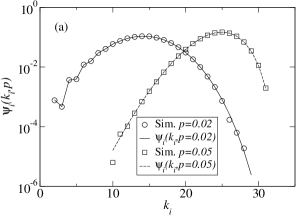
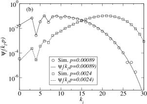
Figure 3: $\psi_{i}(k_{i},p)$ vs. $k_{i}$ calculated both from theory Eq. (6) (curves) and simulations (symbols): (a) $N=32$, $r=3$, and $p\approx 0.02~{}(\bigcirc),0.05~{}(\square)$ with $10^{5}$ realizations per simulation. (b) $N=32$, $r=4$, and $p\approx 0.00089~{}(\bigcirc),0.0024~{}(\square)$ with $10^{4}$ realizations per simulation.

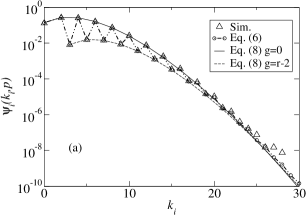
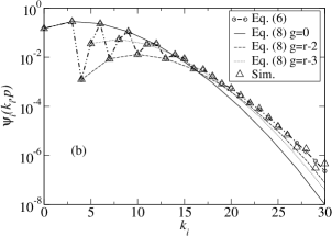
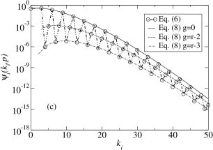
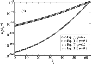
Figure 4: $\psi_{i}(k_{i},p)$ vs. $k_{i}$ from Eq. (6) in the sparse limit (close to percolation), and the sparse approximations $\psi_{i}(k_{i},p,g)$ given in Eq. (8): (a) $N=128,r=3$ and $p$ is adjusted to $\langle k\rangle=4$ (simulations have $10^{6}$ realizations), (b) $N=64,r=4$ and $p$ is adjusted to $\langle k\rangle=6$ ($10^{5}$ realizations), and (c) $N=2048,r=4$ and $p$ is adjusted to $\langle k\rangle=3.5$ (all curves are theoretical). In all plots, the values from Eq. (6) are represented by ($\bigcirc$) connected with the double dot-dashed line, simulations by ($\triangle$), and the approximations $\psi_{i}(k_{i},p,g)$ by thin continuous line for $g=0$, dashed line for $g=r-2$, and dot-dashed line for $g=r-3$. For small systems such as (a) and (b), it is better to use Eq. (7) for $\psi_{i}(k_{i},p,g)$, since the asymptotic limit is still not fully expressed. However, in (c) the size is large enough and displays good asymptotics, given by Eq. (8). (d) $\psi_{i}(k_{i},p)$ vs. $k_{i}$ in the dense limit for $N=64,r=3$ and $p=0.1,0.2$ from Eq. (6) ($\bigcirc$) and the dense approximation Eq. (11)($\square$) (all theoretical results). As $p$ increases the agreement improves.

Figure 3 shows examples of $\psi_{i}(k_{i},p)$ from analytics and simulations, for the general case (“intermediate” $p$), and $r=3,4$; Fig. 4 does the same for the sparse and dense cases (small and large $p$).

In the sparse case, close to the percolation threshold of the hypergraphs, large fluctuations appear in the distribution at relatively small $k_{i}$. This behavior emerges because, at small $p$, the likelihood that hyperedges share multiple nodes (node overlaps) is low, which occurs when $k_{i}$ is not a multiple of $r-1$. To explain this, consider the low density regime when $p\sim\alpha p_{c}$ with $\alpha$ a constant of order $\gtrsim 1$ ($\alpha=1$ is the percolation threshold as derived in Ref. Lopez-projections , with $p_{c}=\left(N\frac{\partial^{2}}{\partial N^{2}}{N\choose r}\right)^{-1}$). In this regime, $\psi_{i}(k_{i},p)$ can in fact be well approximated by using only $\ell=\lceil k_{i}/(r-1)\rceil$, i.e.

$$\psi_{i}(k_{i},p)\approx{N-1\choose k_{i}}Q_{r-1}\left(k_{i},\left\lceil\frac{k_{i}}{r-1}\right\rceil\right)p^{\left\lceil\frac{k_{i}}{r-1}\right\rceil}(1-p)^{{N-1\choose r-1}-\left\lceil\frac{k_{i}}{r-1}\right\rceil};\qquad[p\sim\alpha p_{c}].$$ (7)

The direct calculation of $Q_{r-1}(k_{i},\lceil k_{i}/(r-1)\rceil)$ is addressed in Sec. IV.2. To track whether $k_{i}$ is a multiple of $r-1$, one can introduce $g\equiv\text{mod}(k_{i},r-1)$, where $0\leq g\leq r-2$. If $g=0$, $k_{i}$ is a multiple of $r-1$. On the other hand, when $g\neq 0$, there are $r-1-g$ node overlaps. For very large $N$, $p_{c}\sim\alpha(r-2)!/N^{r-1}$, which together with Stirling’s approximation and $Q(k_{i},\lceil k_{i}/(r-1)\rceil)$ from Sec. IV.2, lead to $\psi_{i}(k_{i},p)\to\psi_{i}(k_{i},p,g)$ in the sparse limit

$$\psi_{i}(k_{i},p,g)\approx N^{g-(r-1)}\frac{e^{-\alpha/(r-1)}}{\left(\left\lceil\frac{k_{i}}{r-1}\right\rceil\right)!}\left(\frac{\alpha}{r-1}\right)^{\lceil k_{i}/(r-1)\rceil}X_{g}\left(r,\left\lceil\frac{k_{i}}{r-1}\right\rceil\right)\qquad\left[p\sim\frac{\alpha(r-2)!}{N^{r-1}}\right],$$ (8)

where

$$X_{g}\left(r,\left\lceil\frac{k_{i}}{r-1}\right\rceil\right)=\left\{\begin{array}[]{ll}1;&\qquad g=0\\ \frac{(r-1)^{2}}{2}\left\lceil\frac{k_{i}}{r-1}\right\rceil\left(\left\lceil\frac{k_{i}}{r-1}\right\rceil-1\right);&\qquad g=r-2\\ \vdots&\qquad\vdots\\ X_{1}\left(r,\left\lceil\frac{k_{i}}{r-1}\right\rceil\right);&\qquad g=1.\end{array}\right.$$ (9)

Also, for the purposes of these approximations, one takes

$$\left\lceil\frac{k_{i}}{r-1}\right\rceil=\left\{\begin{array}[]{ll}\frac{k_{i}}{r-1};&\qquad g=0\\ \frac{k_{i}+1}{r-1};&\qquad g=r-2\\ \vdots&\qquad\vdots\\ \frac{k_{i}+r-1-g}{r-1};&\qquad g=1,\end{array}\right.$$ (10)

which give the correct value of $\lceil k_{i}/(r-1)\rceil$ for the specific $g$ listed. Equation (8) is quite informative. When $g=0$, the degree distribution is strictly Poisson, but when $g\neq 0$, an asymptotic attenuation factor of the form $N^{g-(r-1)}$ appears, which indicates that the probability to observe a single node overlap ($1=r-1-g=r-1-(r-2)$) is reduced by a $1/N$ factor, a 2 node overlap ($2=r-1-g=r-1-(r-3)$) by $1/N^{2}$, etc. The qualitative relevance of this result is that approximations of hypergraphs that consider the hyperedges as non-overlapping when projected onto a graph (or made into a one-mode network of a bipartite network) incur an error of order $N^{-1}$ in $\psi_{i}(k_{i},p)$ in the sparse limit. In Fig. 4(a), (b) and (c), the actual distribution (as given by Eq. (6)) is plotted against simulations, and the curves of Eq. (8) are superimposed for confirmation; one plot is performed on a system size much larger than those available for Monte Carlo simulation, but shows the best adherence to asymptotics. The case $g=0$ is an envelope for the distributions when $N\to\infty$.

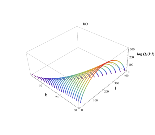
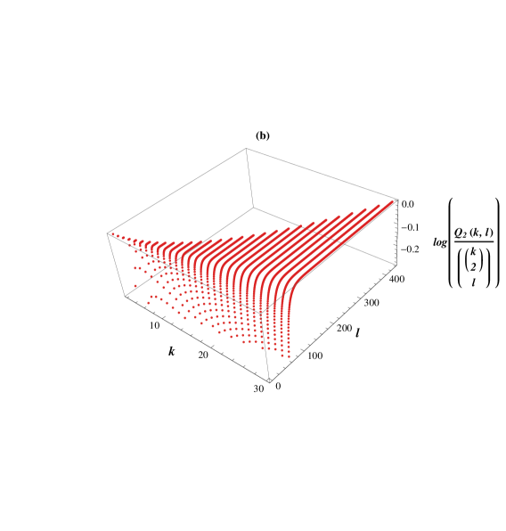
Figure 7: (color online) (a) $\ln Q_{2}(k,\ell)$ vs. $k,\ell$ and (b) $\ln[Q_{2}(k,\ell)/{{k\choose 2}\choose\ell}]$ vs. $k,\ell$. From (b) it is clear that as $\ell$ increases for any $k$, the ratio tends to 1 (with $\log$ going to 0).

In the dense limit, if overlaps are ignored when trying to estimate $\psi_{i}(k_{i},p)$, the error becomes overwhelming. To illustrate this, note that as $p\to 1$ the number of hyperedges visiting $i$ approaches ${N-1\choose r-1}$, and with no overlaps this would lead to a $k_{i}$ approaching $(r-1){N-1\choose r-1}$ which is clearly wrong as in reality $k_{i}$ can be at most $N-1$. With the results in Sec. III.2.4 and, in particular, the realization that for large $\ell_{i}$, $Q_{r-1}(k_{i},\ell_{i})$ can be approximated as ${{k_{i}\choose r-1}\choose\ell_{i}}$ (see Fig. 7(b)), the simple approximation

$$\psi_{i}(k_{i},p)\approx{N-1\choose k_{i}}(1-p)^{{N-1\choose r-1}-{k_{i}\choose r-1}}\qquad[\text{large }p]$$ (11)

for finite and relatively large $p$ becomes satisfactory. This can be obtained by algebraic manipulation and the use of the gaussian approximation for the summand of Eq. (6). Note that the limit $p\to 1$ is correctly obtained: for all $k_{i}<N-1$, the exponent of $1-p$ is positive, and as $p$ approaches 1, $\psi_{i}(k_{i},p)\to 0$; only $k_{i}=N-1$ makes the exponent of $1-p$ equal to zero, producing the result $\psi_{i}(k_{i}=N-1,p=1)\to{N-1\choose N-1}=1$. Figure 4(d) shows examples of the dense estimate Eq. (11) against Eq. (6), which agree well with each other.

To fully specify Eq. (6), it is necessary to determine $Q_{r-1}(k_{i},\ell_{i})$. In order to achieve this, it is important to develop some intuition about the meaning of $Q_{r-1}(k_{i},\ell_{i})$. The case $r=3$ is very useful. Each hyperedge (in this case a triplet) connects $i$ to two other nodes taken out of $\rho(k_{i})$, and clearly all nodes in $\rho(k_{i})$ are visited at least once so that the degree is equal to $k_{i}$. On any two nodes of $\rho(k_{i})$, say $a$ and $b$, the 3-hyperedge that connects them to $i$ acts as an edge between $a$ and $b$. Given that there are $\ell_{i}$ hyperedges available to achieve $k_{i}$, determining $Q_{2}(k_{i},\ell_{i})$ is equivalent to enumerating all distinct labelled graphs of $k_{i}$ nodes and $\ell_{i}$ edges, in which all nodes have degree at least one; there are no isolated nodes. Henceforth, I refer to these graphs as conditioned graphs. In the examples in Fig. 2, the cases contributing to $k_{i}=3$ and $\ell_{i}=2$ are: i) $(a,b)$ and $(b,c)$, ii) $(a,b)$ and $(a,c)$, and iii) $(a,c)$ and $(b,c)$, and to $k_{i}=3$ and $\ell_{i}=3$ is $(a,b)$, $(a,c)$ and $(b,c)$. When the problem is generalized, $Q_{r-1}(k_{i},\ell_{i})$ corresponds to the number of distinct labelled hypergraphs with $k_{i}$ nodes and $\ell_{i}$ hyperedges of rank $r-1$ such that all nodes belong to at least one hyperedge fn-I . In the next section, the calculation of $Q_{2}(k_{i},\ell_{i})$ is tackled through different techniques, leading to the two formulas (Eqns. (17) and (35) where the first one is valid for all $r$).

To conclude this section and relate the model to some concrete applications, I determine $\langle k_{i}\rangle$ and explain its significance in a practical example, which also highlights the importance of the exact results derived here. One can calculate $\langle k_{i}\rangle$ using $P(\boldsymbol{\sigma})$ (later on, this calculation is repeated using $\psi_{i}(k_{i},p)$ and identities relevant to $Q_{r-1}(k_{i},\ell_{i})$). By definition

$$\langle k_{i}\rangle=\sum_{\boldsymbol{\sigma}\in\{\boldsymbol{\sigma}\}_{\rm conf}}k_{i}(\boldsymbol{\sigma})P(\boldsymbol{\sigma})=\sum_{\boldsymbol{\sigma}\in\{\boldsymbol{\sigma}\}_{\rm conf}}\sum_{j=1;j\neq i}^{N}\theta(o_{ij}(\boldsymbol{\sigma}))P(\boldsymbol{\sigma})=\sum_{j=1;j\neq i}^{N}\sum_{\boldsymbol{\sigma}\in\{\boldsymbol{\sigma}\}_{\rm conf}}\theta(o_{ij}(\boldsymbol{\sigma}))P(\boldsymbol{\sigma}).$$ (12)

Concentrating on the sum over $\boldsymbol{\sigma}$

$$\sum_{\boldsymbol{\sigma}\in\{\boldsymbol{\sigma}\}_{\rm conf}}\theta(o_{ij}(\boldsymbol{\sigma}))P(\boldsymbol{\sigma})=\sum_{\boldsymbol{\sigma}\in\{\boldsymbol{\sigma}\}_{\rm conf}}P(\boldsymbol{\sigma})-\sum_{o_{ij}(\boldsymbol{\sigma})=0}P(\boldsymbol{\sigma})=1-\sum_{o_{ij}(\boldsymbol{\sigma})=0}P(\boldsymbol{\sigma}),$$ (13)

where one uses the realization that $\theta(o_{ij}(\boldsymbol{\sigma}))=1$ in all hypergraphs where $o_{ij}\geq 1$, and 0 if $o_{ij}=0$. To determine the last sum, one uses the independence of the hyperedges in Eq. (2), and therefore

$$\sum_{o_{ij}(\boldsymbol{\sigma})=0}P(\boldsymbol{\sigma})=\sum_{\sigma_{1,\dots,r}=0}^{1}p^{\sigma_{1,\dots,r}}(1-p)^{1-\sigma_{1,\dots,r}}\dots\sum_{\sigma_{N-r+1,\dots,N}=0}^{1}p^{\sigma_{N-r+1,\dots,N}}(1-p)^{1-\sigma_{N-r+1,\dots,N}}\\ =(1-p)^{N-2\choose r-2},$$ (14)

where all hyperedges $\sigma_{i_{1},\dots,i_{r}}=0$ when both $i$ and $j$ are among the indices so that $o_{ij}=0$ (there are ${N-2\choose r-2}$ such hyperedges), and the sums over all other $\sigma_{i_{1},\dots,i_{r}}$ produce factors of 1. Since this result is independent of $j$,

$$\langle k_{i}\rangle=\sum_{j=1;j\neq i}^{N}\left[1-(1-p)^{N-2\choose r-2}\right]=(N-1)\left[1-(1-p)^{N-2\choose r-2}\right].$$ (15)

Higher moments can also be calculated this way, but they introduce couplings among indices, and the previous approach becomes much harder. In Sec. IV.1, a more powerful approach is developed making more straightforward the calculation of higher moments. Note that the low density regime $p=\alpha p_{c}$ corresponds to $\langle k_{i}\rangle\sim\alpha$.

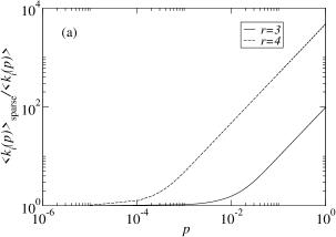
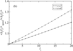
Figure 5: (a) Ratio $\langle k_{i}(p)\rangle_{\rm sparse}/\langle k_{i}(p)\rangle$ versus $p$ calculated via the sparse approximation Eq. (8) with $g=0$ and Eq. (15) for $N=100$. One can quickly see the two quantities deviate considerably even for small $p$. (b) Ratio $\langle k_{i}(\ell_{i})\rangle_{\rm sparse}/\langle k_{i}(\ell_{i})\rangle$ versus $\ell_{i}$ for $N=100$ and $r=3$ and 4, which also shows how rapidly the sparse approximation and the exact results deviate from one another.

To illustrate the relevance of the model in practice, consider the determination of quarantine levels necessary to isolate an individual with an infectious disease. To a first approximation, the quantity of interest here is $\langle k_{i}\rangle$. In a traditional approach with sparse approximate mathematical models, there would be considerable overestimations of quarantine levels because node overlaps are ignored, and thus a friend or colleague that is part of two communities at the same time would be counted twice. When the correct approach is taken, quarantine levels are estimated in a more realistic way. In Fig. 5(a), I present the exact value of the ratio $\langle k_{i}(p)\rangle_{\rm sparse}/\langle k_{i}(p)\rangle$ where $\langle k_{i}(p)\rangle$ is given by Eq. (15) and $\langle k_{i}(p)\rangle_{\rm sparse}=(r-1){N-1\choose r-1}p$ which is the average number of hyperedges connected to node $i$ times the $r-1$ neighbors that each edge contributes. This ratio of averages, which is a measure of how much the sparse approximation differs from the correct value, deviates from 1 very rapidly even for a very small $p$. For a ratio $\langle k_{i}(p)\rangle_{\rm sparse}/\langle k_{i}(p)\rangle$ equal to 2, with $N=100$, $p\approx 0.016$ for $r=3$ and $\approx 3.35\times 10^{-4}$ for $r=4$, which corresponds to an expected number of hyperedges $\langle\ell\rangle\approx 79.3$ for $r=3$ and 52.60 for $r=4$. On a social network this is a very small number of hyperedges, and thus in a quarantine situation, even at this sparse density, the sparse approximation fails suggesting twice as many individuals need to be quarantined than when overlaps are considered. Another way to measure the discrepancy in quarantine levels is to calculate $\langle k_{i}(\ell_{i})\rangle_{\rm sparse}/\langle k_{i}(\ell_{i})\rangle$, which compares for a given node the number of neighbors $k_{i}$ expected in the sparse approximation and in our calculations when the number of hyperedges $\ell_{i}$ connected to the node is given; $\langle k_{i}(\ell_{i})\rangle_{\rm sparse}=(r-1)\ell_{i}$ whereas $\langle k_{i}(\ell_{i})\rangle=(N-1)\left(1-{{N-2\choose r-1}\choose\ell_{i}}/{{N-1\choose r-1}\choose\ell_{i}}\right)$ which can be calculated from the ratio between Eqs. (45) and (55) in Sec. IV.1. Here (see Fig. 5(b)), the ratio also moves away from 1 quickly, and by $\ell_{i}=20$ it overestimates the number of neighbors by $20\%$ for $r=3$ and $32\%$ for $r=4$. These examples show that, essentially, in order to properly account for node neighbors in systems with group structure, node overlaps can hardly be ignored, and the approach presented here becomes necessary.

Our random hypergraph model (considering also results in Ref. Lopez-projections ) has other domains of application, such as being a source of random null models for studies of data-constructed networks. To take an example, if one considers a network structure given directly by data, such as a metabolic network, certain structural features of the network can be compared to random null models of the network to determine if they are statistically rare. If so, such features are potentially relevant biologically and may warrant further study. Furthermore, if the data-constructed model has a one-mode network representation believed to be a useful simplification of the full hypergraph or bipertite network model (e.g., because it lends itself to the use of some technique best defined only on graphs), our framework provides the most complete way to determine the statistics of the associated one-mode random null model, and hence would prove useful for intepretation and analysis in this approach.

III Calculations of $Q_{r-1}(k,\ell)$

To determine $Q_{r-1}(k_{i},\ell_{i})$, I proceed by focusing on the enumeration of the conditioned graphs/hypergraphs mentioned above. To avoid confusion, it is important to emphasize that the graphs and hypergraphs considered in this section are not those in $\{\boldsymbol{\sigma}\}_{\rm conf}$, but instead are tools to determine $Q_{r-1}$ and, if desired, can be interepreted directly in the context of $\{\boldsymbol{\sigma}\}_{\rm conf}$ fn-I , but it is not necessary. The nodes are labelled, consistent with the selection of sets $\rho(k_{i})$ which are also composed of labelled nodes. In the calculations of this section, given a choice $\rho(k_{i})$ with $k_{i}$ nodes and $\ell_{i}$ hyperedges of rank $r-1$, the node $i$ is irrelevant and therefore the subindex $i$ is dropped.

III.1 Inclusion-Exclusion formula

The combinatorial coefficient $Q_{r-1}(k,\ell)$ can be determined via the inclusion-exclusion principle of combinatorics Riordan . The idea behind this principle is to count the number of elements in a set that satisfies certain conditions through a series of alternative overcounts and undercounts. Focusing on $Q_{2}(k,\ell)$ as the enumeration of conditioned graphs, a simple overcount of the conditioned graphs is ${{k\choose 2}\choose\ell}$, the number of graphs with $k$ nodes and $\ell$ edges, where there are ${k\choose 2}$ places to locate $\ell$ edges. This overcounts $Q_{2}(k,\ell)$ because it ignores the condition of all nodes being connected to at least one edge. If the configurations in which at least one node is not connected are taken away from the previous enumeration, the correct result is obtained. To approach this, one makes a first correction by taking away ${k\choose k-1}{{k-1\choose 2}\choose\ell}$, which counts all choices of $k-1$ nodes picked out of $k$ multiplied by the number graphs formed with $k-1$ nodes and $\ell$ edges. This step has now eliminated all configurations that have nodes disconnected, but has eliminated multiple times all graphs in which two or more nodes are not connected to an edge. To correct for this, it is necessary to add ${k\choose k-2}{{k-2\choose 2}\choose\ell}$. Once again there are unwanted graphs in this count which require further correction. It is straightforward to continue this until the point when the choice of $m$ nodes chosen out of $k$ is small enough that ${m\choose 2}<\ell$, at which point the sequence stops. These considerations lead to the expression

$$Q_{2}(k,\ell)=\sum_{m=0}^{k}(-1)^{k-m}{k\choose m}{{m\choose 2}\choose\ell}.$$ (16)

The extension to arbitrary $r$ is direct, producing

$$Q_{r-1}(k,\ell)=\sum_{m=0}^{k}(-1)^{k-m}{k\choose m}{{m\choose r-1}\choose\ell}.$$ (17)

In terms of direct calculation, this formula is useful in producing an exact numerical result, but it is not so easy to interpret on the basis of $k$ and $\ell$, and some calculations that depend on it become difficult due to the alternating signs (e.g. asymptotics).

III.2 Assembly of $Q_{2}(k,\ell)$

An alternative to inclusion-exclusion is that of graph assembly. In this section, I explain how to compute $Q_{r-1}(k,\ell)$ with $r=3$ through assembly. The extension to arbitrary $r$ is explained in Sec. III.3, and though it is straightforward, it is admittedly cumbersome. Nevertheless, the picture developed here is more intuitive than inclusion-exclusion, and opens the possibility to study the properties of $Q_{r-1}(k,\ell)$ further. To develop the procedure to count assemblies leading to the conditioned graphs, small examples are presented where $\ell$ is close to its minimum possible value for given $k$. These examples exhibit all the aspects necessary to deal with the general $Q_{2}(k,\ell)$ case, which is studied in Sec. III.2.4.

III.2.1 Preliminaries and simple examples. Types of edges

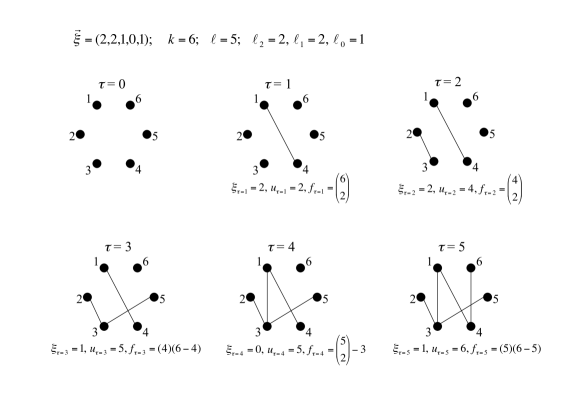
Figure 6: Assembly of a conditioned graph contributing to $Q_{2}(k,\ell)$ for $k=6,\ell=5$. In this example, the assembly history is given by $\vec{\xi}=(2,2,1,0,1)$, representing the fact that the edges added are, in order of appearance, of types $\ell_{2},\ell_{2},\ell_{1},\ell_{0},\ell_{1}$. At each assembly step $\tau$, the type of edge $\xi_{\tau}$, total number of used (discovered) nodes $u_{\tau}$, and combinatorial factor $f_{\tau}$ are given. The total combinatorics of assemblies with this same history $\vec{\xi}=(2,2,1,0,1)$ is given by Eq. (24).

In order to determine $Q_{2}(k,\ell)$ via assembly, one begins with $k$ isolated nodes and adds edges, totalling $\ell$, so that every node is connected to an edge. Once two nodes have been connected by an edge, they cannot be connected again (i.e., multigraphs are not allowed). To find all distinct graphs that contribute to $Q_{2}(k,\ell)$, one first needs to determine all possible ways to assemble those graphs. The number of distinct assemblies is larger than $Q_{2}(k,\ell)$, but is trivially corrected to yield $Q_{2}(k,\ell)$, as explained below. For the assembly process, the critical ingredient is knowledge of the number of distinct ways in which a given edge can enter into the graph. I now proceed to describe this enumeration (refer throughout this section to Fig. 6 for a specific example of assembly, along with the relevant notation).

Consider the initial state of $k$ isolated nodes. At this initial step of the process, there are ${k\choose 2}$ possible pairs of nodes in which an edge can be placed. After the first step of edge addition, 2 nodes become used (or discovered). Let us define the vector $\vec{\xi}$ which characterizes the edge addition process. This vector has length $\ell$ (i.e. its dimension $\dim\vec{\xi}=\ell$). The $\tau$-th component of the vector, $\xi_{\tau}$, is the number of nodes that are discovered by the addition of the $\tau$-th edge in the assembly; for the first step, $\xi_{\tau=1}=2$. Another useful definition is $u_{\tau}$, the number of nodes discovered up to step $\tau$. In all assemblies, $\xi_{\tau=1}=2$ and $u_{\tau=1}=2$. After the first edge is added in one of the possible ${k\choose 2}$ places on the graph, there are in total ${k\choose 2}$ possible distinct graphs.

Each additional added edge generates an enumeration depending on the nodes that are involved in that edge. To illustrate this, consider the possibilities when adding the second edge, i.e. $\tau=2$. The first possibility corresponds to edge $\tau=2$ being used to discover two new nodes out of the remaining $k-2$ undiscovered nodes, among which there are ${k-2\choose 2}$ possible node pairs. This leads to a total of ${k\choose 2}{k-2\choose 2}$ distinct graph assemblies, where $u_{\tau=2}=4$. In $\vec{\xi}$, component $\xi_{\tau=2}=2$ because the second edge discovers 2 new nodes. The second possibility for $\tau=2$ corresponds to adding an edge that connects one of the two nodes already in use to one of the $k-2$ undiscovered nodes. This leads to ${k\choose 2}(2(k-2))$ distinct graph assemblies because the second edge has 2 choices among discovered nodes and $k-2$ choices among undiscovered nodes; in this case $u_{\tau=2}=3$ and $\xi_{\tau=2}=1$.

The condition of visiting all $k$ nodes at least once imposes in turn conditions of the numbers of edges with $\xi_{\tau}$ equal to 1 or 2. It is convenient to introduce notation for these edges. If the addition of an edge at a given step $\tau$ discovers two unused nodes, this edge is counted into $\ell_{2}$ and is described as being a type $\ell_{2}$ edge. On the other hand, if at $\tau$ an edge connects a node already discovered in a step $<\tau$ to an undiscovered node, it counts into $\ell_{1}$ and is referred to as a type $\ell_{1}$ edge. For an arbitrary step $\tau$ in the assembly, type $\ell_{2}$ edges are associated with a factor ${k-u_{\tau-1}\choose 2}$ in the enumeration because they connect 2 out of the remaining $k-u_{\tau-1}$ undiscovered nodes; type $\ell_{1}$ edges are associated with a factor $u_{\tau-1}(k-u_{\tau-1})$ because they connect one of the $u_{\tau-1}$ discovered nodes to one of the $k-u_{\tau-1}$ undiscovered nodes. The counts $\ell_{1}$ and $\ell_{2}$ are part of the total number of edges $\ell$. Another kind of edge is possible, which connects two nodes already discovered; these edges are counted by $\ell_{0}$ and referred to as type $\ell_{0}$ edges (the 0 refers to the fact that their introduction does not contribute to $k$ because they do not discover new nodes). Below, I will give examples of the enumeration for type $\ell_{0}$ edges. The relation between $\ell_{2},\ell_{1},\ell_{0}$ and $k,\ell$ is summarized in the equations

$$\ell = \ell_{2}+\ell_{1}+\ell_{0}$$ (18)

$$k = 2\ell_{2}+\ell_{1},$$ (19)

where only integer non-negative solutions are allowed.

At this point, it is useful to make a few simple calculations that illustrate the ideas just described. First, consider $k$ even, and let us assemble a conditioned graph with the minimum number of edges possible. Clearly, $\ell=k/2$, where each edge must connect a new pair of undiscovered nodes until all nodes are discovered, and therefore $\ell=\ell_{2}=k/2$. Hence, there are $\prod_{a=1}^{k/2}{k-2(a-1)\choose 2}$ distinct assemblies and

$$Q_{2}(k,\ell=k/2)=\frac{1}{\left(\frac{k}{2}\right)!}\prod_{a=1}^{k/2}{k-2(a-1)\choose 2}=\frac{k!}{2^{k/2}(k/2)!}\qquad[\text{$k$ even}]$$ (20)

distinct conditioned graphs. The $(k/2)!$ in the denominator comes from the fact that the order in which the $\ell=k/2$ edges are chosen is irrelevant to the assembled graph, and thus their permutations must be taken away. In $\vec{\xi}$ notation, $\vec{\xi}=(2,\dots,2)$, i.e., $\xi_{\tau}=2$ for all $\tau$, and $\dim\vec{\xi}=\ell_{2}=k/2$. In this example, $\vec{\xi}$ is unique.

The next example to consider is when $k$ is an odd number and $\ell$ is minimal ($\ell=\lceil k/2\rceil=(k+1)/2$ in this case). To assemble such conditioned graphs, any one of the $k$ nodes must be reused exactly once to achieve the condition of all nodes being connected to at least one edge, and thus $\ell_{1}=1$ and $\ell_{2}=(k-1)/2$. As before, one chooses the first edge out of ${k\choose 2}$ possibilities, and from $\tau=2$ and beyond the possibility to add the single edge of type $\ell_{1}$ is available. If this edge is added in step $\tau=b$, and summing over all possible values of $b$, the enumeration becomes

$$Q_{2}(k,\ell=(k+1)/2)=\\ \frac{1}{\left(\frac{k+1}{2}\right)!}\sum_{b=2}^{(k+1)/2}(2(b-1))(k-2(b-1))\prod_{a_{1}=1}^{b-1}{k-2(a_{1}-1)\choose 2}\prod_{a_{2}=b+1}^{(k+1)/2}{k-2(a_{2}-1)+1\choose 2}\\ =\frac{k!}{2^{(k-1)/2}\left(\frac{k-3}{2}\right)!}\qquad[\text{$k$ odd}],$$ (21)

because for given $b$ there are ${k\choose 2}{k-2\choose 2}\dots k-2(b-2)\choose 2$ ways to assemble the first $2(b-1)$ nodes using type $\ell_{2}$ edges, $(2(b-1))(k-2(b-1))$ possible ways to introduce the type $\ell_{1}$ edge, and after that, there are still $k-2(b-1)-1$ remaining nodes that are connected in ${k-2(b-1)-1\choose 2}\dots 2\choose 2$ possible ways ($k-2(b-1)-1$ is even). The denominator $\left(\frac{k+1}{2}\right)!$ corrects for order in the permutations of the edge addition. In $\vec{\xi}$ notation, each value of $b$ is associated with a $\vec{\xi}$ in which $\xi_{\tau=b}=1$ and $\xi_{\tau\neq b}=2$, and $\dim\vec{\xi}=(k+1)/2$. In this example, unlike before, $\vec{\xi}$ is not unique; there are $(k-1)/2$ different $\vec{\xi}$, one for each choice of $b$ between 2 and $(k+1)/2$.

For the last example, consider $k$ even and $\ell=k/2+1$ (no longer minimal). In this situation, one can either: i) connect all pairs of nodes by use of $\ell_{2}=k/2$ edges while at some step $\tau=c$ use a single type $\ell_{0}$ edge to connect two nodes of the $u_{\tau-1=c-1}$ that have already been discovered up to step $\tau-1=c-1$, or ii) connect $k-2$ nodes via $\ell_{2}=(k-2)/2$ edges, and also use $\ell_{1}=2$ edges at steps $\tau=b_{1}$ and $\tau=b_{2}$ to connect the remaining 2 nodes; the two cases are mutually exclusive. Therefore, considering all possible $b_{1},b_{2},c$,

$$Q_{2}\left(k,\ell=\frac{k}{2}+1\right)=\frac{1}{\left(\frac{k}{2}+1\right)!}\\ \left[\sum_{b_{1}=2}^{k/2}(2(b_{1}-1))(k-2(b_{1}-1))\sum_{b_{2}=b_{1}+1}^{k/2+1}(2(b_{2}-1)-1)(k-2(b_{2}-1)+1)\right.\\ \prod_{a_{1}=1}^{b_{1}-1}{k-2(a_{1}-1)\choose 2}\prod_{a_{2}=b_{1}+1}^{b_{2}-1}{k-2(a_{2}-1)+1\choose 2}\prod_{a_{3}=b_{2}+1}^{k/2+1}{k-2(a_{3}-1)+2\choose 2}\\ \left.+\sum_{c=2}^{k/2}\left({2c\choose 2}-c\right)\prod_{a_{1}=2}^{k/2}{k-2(a_{1}-1)\choose 2}\right]=\frac{k!}{2^{k/2}\left(\frac{k}{2}-2\right)!}\left(\frac{3k+4}{6}\right)\qquad[\text{$k$ even}].$$ (22)

The first set of sums in the square brackets enumerate the cases of two separate instances of visiting one used node ($\ell_{2}=(k-2)/2,\ell_{1}=2,\ell_{0}=0$), and the second sum enumerates the cases when one edge is placed between two previously used nodes ($\ell_{2}=k/2,\ell_{1}=0,\ell_{0}=1$). For the second sum, note that any type $\ell_{0}$ edge placed between two nodes already present occurs when 4 or 6 or … $k$ nodes have been used for the first time. At each of these steps, the number of choices is ${4\choose 2}-2,{6\choose 2}-3,\dots,{k\choose 2}-k/2$, which account for the number of possible edges between the nodes present minus the edges that have been placed. Generally, for a type $\ell_{0}$ edge introduced at step $\tau$, the factor associated with its enumeration is ${u_{\tau-1}\choose 2}-(\tau-1)$. Note that for such an edge $u_{\tau}=u_{\tau-1}$. Once again, the prefactor $1/(1+k/2)!$ accounts for eliminating the permutations among overall edge placement order. In $\vec{\xi}$ notation, there are now two kinds of vectors: for $\ell_{2}=(k-2)/2,\ell_{1}=2,\ell_{0}=0$, there are ${(k-1)/2\choose 2}$ distinct $\vec{\xi}$, one for each $\xi_{\tau=b_{1}}=1,\xi_{\tau=b_{2}}=1,\xi_{\tau\neq b_{1},b_{2}}=2$; for $\ell_{2}=k/2,\ell_{1}=0,\ell_{0}=1$ there are $(k-2)/2$ vectors $\vec{\xi}$, one for each case of $\xi_{\tau=c}=0,\xi_{\tau\neq c}=2$, where $c\geq 2$ because in this example there must be at least 2 edges (and 4 nodes) before any type $\ell_{0}$ can be introduced.

It is clear that in all examples above, one can use a shorthand to represent the sums for the assemblies by using $\vec{\xi}$. Thus, $Q_{2}(k,\ell)=(\ell!)^{-1}\sum_{\vec{\xi}}C(\vec{\xi})$ where $C(\vec{\xi})$ is the combinatorial factor associated with an assembly history $\vec{\xi}$, and the $\vec{\xi}$ are chosen to satisfy the given $k$ and $\ell$.

III.2.2 Setup of the $Q_{2}(k,\ell)$ calculation

The three calculations above exhibit all types of edges in the assembly process: edges that visit two new nodes, edges that visit one new node and a previously visited node, and edges that visit two already visited nodes. Clearly, the kinds and numbers of edges used are constrained to satisfy the definition of $Q_{2}(k,\ell)$ as explained below. The function that each edge performs (type $\ell_{2},\ell_{1}$ or $\ell_{0}$) depends on the step at which it is added, which is equivalent to assuming that edges are distinguishable. The advantage of making this distinguishability available is that it converts the counting of $Q_{2}(k,\ell)$ into a process that is tractable, i.e., it provides rules to count all possibilities. However, if one looks at the final product of the assembly, the relevant conditioned graphs of $Q_{2}(k,\ell)$, it would be impossible to determine which edge came first or what function it performed (this is the reason why one divides $\sum_{\vec{\xi}}C(\vec{\xi})$ by $\ell!$). Essentially, $Q_{2}(k,\ell)$ is calculated by first enumerating all possible assemblies that lead to the conditioned graphs, and then taking away the edge permutations.

As it was shown in Eq. (22), there are multiple choices of $\ell_{0},\ell_{1},\ell_{2}$ for given $k$ and $\ell$. Given that in $Q_{2}(k,\ell)$, $k$ and $\ell$ are specified, it is necessary to express the conditions on $\ell_{0},\ell_{1},\ell_{2}$ as functions of $k$ and $\ell$. But one cannot solve for all three $\ell_{0},\ell_{1},\ell_{2}$ from Eqs. (18) and (19). However, it is possible to solve for $\ell_{1},\ell_{2}$ by focusing on $\ell-\ell_{0}$ and $k$. The solution is $\ell_{2}=k-(\ell-\ell_{0})$ and $\ell_{1}=2(\ell-\ell_{0})-k$. By taking $\ell_{0}$ as a free parameter, and running over all its possible values, all triplets $\ell_{0},\ell_{1},\ell_{2}$ are uniquely specified. All that remains is to determine the allowed range for $\ell_{0}$ which emerges from determining the minimum and maximum $\ell_{1}+\ell_{2}$ ($=\ell-\ell_{0}$) necessary to visit $k$ nodes, while keeping in mind that $\ell_{2}\geq 1$ since the first edge is always type $\ell_{2}$: the minimum occurs when $\ell_{2}=\left\lfloor\frac{k}{2}\right\rfloor$ and $\ell_{1}=k-2\left\lfloor\frac{k}{2}\right\rfloor$ (which gives $\ell_{1}=0$ or 1) so $\ell_{1}+\ell_{2}=\left\lceil\frac{k}{2}\right\rceil$; the maximum occurs for $\ell_{2}=1$ and $\ell_{1}=k-2$ with $\ell_{1}+\ell_{2}=k-1$. Therefore, $\left\lceil\frac{k}{2}\right\rceil\leq\ell_{1}+\ell_{2}\leq k-1$ leading to $\ell-\left\lceil\frac{k}{2}\right\rceil\geq\ell_{0}\geq\ell-(k-1)$. For each unique triplet $\ell_{0},\ell_{1},\ell_{2}$, one can define the number of conditioned graph assemblies $F(\ell_{2},\ell_{1},\ell_{0})$, and

$$Q_{2}(k,\ell)=\sum_{\ell_{0}=\ell-(k-1)}^{\ell-\left\lceil\frac{k}{2}\right\rceil}F(\ell_{2},\ell_{1},\ell_{0})=\sum_{\ell_{0}=\ell-(k-1)}^{\ell-\left\lceil\frac{k}{2}\right\rceil}\sum_{\vec{\xi}\in\{\vec{\xi}(\ell_{2},\ell_{1},\ell_{0})\}_{\rm conf}}F(\vec{\xi}),$$ (23)

where $\{\vec{\xi}(\ell_{2},\ell_{1},\ell_{0})\}_{\rm conf}=\{\vec{\xi}\}_{\rm conf}$ corresponds to the set of all allowed histories $\vec{\xi}$ consistent with $\ell_{0},\ell_{1},\ell_{2}$. Each $F(\vec{\xi})$ has the form

$$F(\vec{\xi})=(\ell!)^{-1}C(\vec{\xi})=(\ell!)^{-1}\prod_{\tau=1}^{\ell}f_{\tau}(u_{\tau-1},\xi_{\tau})$$ (24)

where $f_{\tau}(u_{\tau-1},\xi_{\tau})$ corresponds to the combinatorial assembly factor associated with the addition of the edge of type $\xi_{\tau}$ at step $\tau$, at which point the number of discovered nodes is $u_{\tau-1}$. As stated before, $f_{\tau}(u_{\tau-1},\xi_{\tau}=2)={k-u_{\tau-1}\choose 2}$, $f_{\tau}(u_{\tau-1},\xi_{\tau}=1)=u_{u_{\tau-1}}(k-u_{\tau-1})$, and $f_{\tau}(u_{\tau-1},\xi_{\tau}=0)={u_{\tau-1}\choose 2}-(\tau-1)$. The number of used nodes up to step $\tau$ is given by

$$u_{\tau-1}=\sum_{\tau^{\prime}=1}^{\tau-1}\xi_{\tau^{\prime}},$$ (25)

which completes the calculation.

However, given that calculating $Q_{2}(k,\ell)$ involves summing over all possible $\vec{\xi}$, further specification is possible with more concrete results. Below, the calculation of $F(\ell_{2},\ell_{1},\ell_{0})$ is tackled in steps by first addressing $F(\ell_{2},\ell_{1},\ell_{0}=0)$ and then using this result to introduce $\ell_{0}$ edges and complete the calculation of $Q_{2}(k,\ell)$.

III.2.3 Calculation of $F(\ell_{2},\ell_{1},\ell_{0}=0)$

When $\ell_{0}=0$, only the combinatorics of $\ell_{1}$ and $\ell_{2}$ edges are needed. It is useful to introduce the redefinition $(\vec{\xi},\tau)\to(\vec{h},t)$ in this case (the reason becomes clear in the next Sec.). In this notation $\dim\vec{h}=\ell_{2}+\ell_{1}$, and each component $h_{t}$ can only be 1 or 2. The difference between two histories $\vec{h}$ and $\vec{h}^{\prime}$ with equal $\ell_{1}$ and $\ell_{2}$ is found in the specific steps $t$ in which $h_{t}=1$, i.e., the steps in which the type $\ell_{1}$ edges are introduced. It is then convenient to define a set $\{b_{1},\dots,b_{\ell_{1}}\}$ corresponding to the steps $t$ of the first, second, …, $\ell_{1}$ introductions of type $\ell_{1}$ edges, and a counter $\lambda$ from 0 to $\ell_{1}$. For a concrete $\vec{h}$, for $\lambda=1$ there is an associated step $t=b_{1}$. The conditioned graph enumeration due to type $\ell_{2}$ edges up to $t=b_{1}-1$ is $\prod_{a_{1}=1}^{b_{1}-1}{k-2(a_{1}-1)\choose 2}$ and at $t=b_{1}$ the new factor $2(b_{1}-1)(k-2(b_{1}-1))$ comes in. Between the $\lambda-1$ and $\lambda$ edges of type $\ell_{1}$, that is steps $b_{\lambda-1}+1\leq t\leq b_{\lambda}-1$, enumeration due to type $\ell_{2}$ edges is $\prod_{a_{\lambda}=b_{\lambda-1}+1}^{b_{\lambda}-1}{k-2(a_{\lambda}-1)+(\lambda-1)\choose 2}$, and at $t=b_{\lambda}$ there is a new factor $(2(b_{\lambda}-1)-(\lambda-1))(k-2(b_{\lambda}-1)+(\lambda-1))$. These considerations lead to the expression

$$F(\ell_{2},\ell_{1},\ell_{0}=0)=\equiv F^{(0)}(\ell_{2},\ell_{1})=\frac{1}{(\ell_{2}+\ell_{1})!}\sum_{b_{1}=2}^{\ell_{2}+1}[2(b_{1}-1)][k-2(b_{1}-1)]\prod_{a_{1}=1}^{b_{1}-1}{k-2(a_{1}-1)\choose 2}\dots{\\ }\sum_{b_{\lambda}=t_{\lambda-1}+1}^{\ell_{2}+\lambda}[2(b_{\lambda}-1)-(\lambda-1)][k-2(b_{\lambda}-1)+(\lambda-1)]\prod_{a_{\lambda}=b_{\lambda-1}+1}^{b_{\lambda}-1}{k-2(a_{\lambda}-1)+(\lambda-1)\choose 2}\dots{\\ }\sum_{b_{\ell_{1}}=b_{\ell_{1}-1}+1}^{\ell_{2}+\ell_{1}}[2(b_{\ell_{1}}-1)-(\ell_{1}-1)][k-2(b_{\ell_{1}}-1)+(\ell_{1}-1)]\prod_{a_{\ell_{1}}=b_{\ell_{1}-1}+1}^{b_{\ell_{1}}-1}{k-2(a_{\ell_{1}}-1)+(\ell_{1}-1)\choose 2}\\ \prod_{a_{\ell_{1}+1}=b_{\ell_{1}}+1}^{\ell_{2}+\ell_{1}}{k-2(a_{\ell_{1}+1}-1)+\ell_{1}\choose 2},$$ (26)

where the sums in Eq. (26) reflect all possible ways to choose the set of $b_{\lambda}$.

Equation (26) can be evaluated by noting that the factors due to $\ell_{2}$ edges together with the factors of form $[k-2(b_{\lambda}-1)+(\lambda-1)]$ within the type $\ell_{1}$ enumeration combine to the factorial $k!=(2\ell_{2}+\ell_{1})!$. The denominators coming from the $\ell_{2}$ factors produce $2^{\ell_{2}}$. What remains is the sum of products of the form $[2(b_{\lambda}-1)-(\lambda-1)]$ which come from type $\ell_{1}$ edges, and counts the ways to pick nodes from those that have been discovered in steps previous to $t=b_{\lambda}$, for all $\lambda\leq\ell_{1}$. Hence, one can write

$$F^{(0)}(\ell_{2},\ell_{1})=\frac{k!}{2^{\ell_{2}}(\ell_{2}+\ell_{1})!}A_{1}(\ell_{2},\ell_{1})$$ (27)

where

$$A_{1}(\ell_{2},\ell_{1})\equiv\sum_{b_{1}=2}^{\ell_{2}+1}\sum_{b_{2}=b_{1}+1}^{\ell_{2}+2}\dots\sum_{b_{\ell_{1}}=b_{\ell_{1}-1}+1}^{\ell_{2}+\ell_{1}}[2(b_{1}-1)][2(b_{2}-1)-1]\dots[2(b_{\ell_{1}}-1)-(\ell_{1}-1)].$$ (28)

Equation (27) states that the number of ways to assemble the $k$ nodes when $\ell_{0}=0$ is proportional to the permutations of the nodes and the number of choices in which single previously used nodes can be picked (as $\ell_{1}$ edges are introduced). In $\vec{h}$ notation, $A_{1}(\ell_{2},\ell_{1})$ can be written as

$$A_{1}(\ell_{2},\ell_{1})=\sum_{\vec{h}\in\{\vec{h}(\ell_{2},\ell_{1})\}_{\rm conf}}A_{1}(\vec{h})=\sum_{\vec{h}\in\{\vec{h}(\ell_{2},\ell_{1})\}_{\rm conf}}\prod_{b\in\{t|h_{t}=1\}}u_{b},$$ (29)

where (with a slight abuse of notation) $b$ is an element of $\{t|h_{t}=1\}$, the set of all steps in assembly $\vec{h}$ at which a type $\ell_{1}$ edge is added. In $\vec{h}$ notation,

$$F^{(0)}(\ell_{2},\ell_{1})=\sum_{\vec{h}\in\{\vec{h}\}_{\rm conf}}F^{(0)}(\vec{h})=\frac{k!}{2^{\ell_{2}}(\ell_{2}+\ell_{1})!}\sum_{\vec{h}\in\{\vec{h}\}_{\rm conf}}A_{1}(\vec{h}).$$ (30)

To develop some intuition about $F^{(0)}(\ell_{2},\ell_{1})$, it is useful to make reference to a few examples: if $\ell_{2}=1$ and thus $\ell_{1}=k-2$, $F^{(0)}(\ell_{2},\ell_{1})$ is the number of distinct realizations of invasion percolation without trapping, where the initial seed is an edge (of indistinguishable nodes). For $\ell_{2}>1$, $F^{(0)}(\ell_{2},\ell_{1})$ counts a forest of $\ell_{2}$ of these invasion percolation trees (the trees never coalesce).

III.2.4 Introducing $\ell_{0}>0$ and full $Q_{2}(k,\ell)$

To introduce an edge of type $\ell_{0}$, there must be nodes already used and, in addition, pairs of them that have not been directly connected by another edge. These unconnected node pairs are vacancies. The combinatorics of type $\ell_{0}$ edges require counting the vacancies available as the conditioned graph assembly progresses. The availability of vacancies is restricted by the assembly sequence $\vec{h}$. For instance, consider the first two steps of any assembly. After the first edge of type $\ell_{2}$, the second edge can only be type $\ell_{1}$ or $\ell_{2}$, but not type $\ell_{0}$ because there are no vacancies in the graph yet. Using the notation for steps applied when $\ell_{0}$, the first step at which a type $\ell_{0}$ edge can be introduced is right before $t=3$ since there would be four vacancies if the second edge is type $\ell_{2}$ or one vacancy if it is type $\ell_{1}$ (the distinction between $\vec{h},t$ and $\vec{\xi},\tau$ becomes more evident in this section, where $t$ can be used to describe the equations for the full assembly including type $\ell_{0}$ edges, even though $t$ only counts steps that add nodes, whereas $\tau$ counts every edge addition).

Edges of type $\ell_{0}$ can be placed in any step $t$ of the sequence $\vec{h}$ where there are available vacancies, and to obtain the full enumeration, all possible placings must be counted. Fortunately, even though placing a type $\ell_{0}$ edge is conditional on the vacancies created by $\ell_{2}$ and $\ell_{1}$, the opposite is not true, i.e., placings of $\ell_{1}$ and $\ell_{2}$ are unaffected by $\ell_{0}$, and thus the results of $F^{(0)}(\ell_{2},\ell_{1})$ can be used here. This is because the combinatorics of type $\ell_{1},\ell_{2}$ edges only depend on the numbers of used and unused nodes, and type $\ell_{0}$ edges have no effect on those.

Following the previous description, it makes sense to introduce $\vec{v}=(v_{1},v_{2},\dots,v_{\ell_{1}+\ell_{2}})$, the vacancies available due to the addition of type $\ell_{1}$ and $\ell_{2}$ edges, at the respective steps $t=1,2,\dots,\ell_{1}+\ell_{2}$ of $\vec{h}$ (clearly $\vec{v}$ is a function of $\vec{h}$). These are the vacancies where type $\ell_{0}$ edges can be placed. The values of $v_{t}$ are defined such that they are not affected by the addition of type $\ell_{0}$ edges. To track type $\ell_{0}$ edges, one defines $\vec{n}=(n_{1},n_{2},n_{3},\dots,n_{\ell_{1}+\ell_{2}})$, the number of edges type $\ell_{0}$ placed, respectively, immediately after $t=1,2,3,\dots,\ell_{1}+\ell_{2}$ edges of type $\ell_{1}$ and $\ell_{2}$ have been added (to be clear, at step $t$, an edge of type $\ell_{2}$ or $\ell_{1}$ is added, leading to $v_{t}$, and before the next step $t+1$, $n_{t}$ edges of type $\ell_{0}$ are added). Both $v_{1}$ and $n_{1}$ are equal to zero because there are no vacancies created with the first edge addition and thus it is valid to omit them from $\vec{n}$ and $\vec{v}$ if desired. To determine the combinatorial weight of any particular sequence of $\ell_{0}$ placings, edges can choose among the available vacancies: at step $t=2$, there are $v_{2}$ vacancies, and so $0\leq n_{2}\leq v_{2}$, which can be done in $\frac{v_{2}!}{(v_{2}-n_{2})!}$ ways (keeping in mind the edges are considered distinguishable while being assembled); at $t=3$, there are $v_{3}-n_{2}$ vacancies, and $0\leq n_{3}\leq v_{3}-n_{2}$, with combinatorial weight $(v_{3}-n_{2})!/(v_{3}-n_{2}-n_{3})!$; etc. Therefore, the number of combinations for the sequences $\vec{v}$ and $\vec{n}$ are

$$A_{0}(\vec{n},\vec{v}(\vec{h}))=\prod_{t=2}^{\ell_{1}+\ell_{2}}\frac{\left(v_{t}-\sum_{t^{\prime}=2}^{t-1}n_{t^{\prime}}\right)!}{\left(v_{t}-\sum_{t^{\prime}=2}^{t}n_{t^{\prime}}\right)!};\qquad\left[\text{constrained to }\ell_{0}=\sum_{t=2}^{\ell_{1}+\ell_{2}}n_{t}\right].$$ (31)

For a given sequence $\vec{v}$, all allowed $\vec{n}$ contribute to $Q_{2}(k,\ell)$, and therefore it is necessary to sum over all $\vec{n}$ subject to the condition in the brackets. Thus, to each term $A_{1}(\vec{h})$, one multiplies the factor

$$\sum_{\vec{n}}A_{0}(\vec{n},\vec{v}(\vec{h}))=\sum_{[n_{2}+\dots+n_{\ell_{1}+\ell_{2}}=\ell_{0}]}\prod_{t=2}^{\ell_{1}+\ell_{2}}\frac{\left(v_{t}-\sum_{t^{\prime}=2}^{t-1}n_{t^{\prime}}\right)!}{\left(v_{t}-\sum_{t^{\prime}=2}^{t}n_{t^{\prime}}\right)!},$$ (32)

where the notation of the sum implies summing over all combinations of $n_{t}$ that satisfy the constraint $n_{2}+\dots+n_{\ell_{1}+\ell_{2}}=\ell_{0}$. To fully specify the previous, and recalling Eq. (25), $v_{t}$ is given by

$$v_{t}={u_{t}\choose 2}-t,$$ (33)

which has already been mentioned in the discussions of Eqs. (22) and (24).

These results can now be put together in a single expression. From Eqns. (30) and (32)

$$F(\ell_{2},\ell_{1},\ell_{0})=\frac{k!}{2^{\ell_{2}}(\ell_{2}+\ell_{1}+\ell_{0})!}\sum_{\vec{h}}A_{1}(\vec{h})\sum_{\vec{n}}A_{0}(\vec{n},\vec{v}(\vec{h})).$$ (34)

With the use of Eqn. (23) and the relations between $k,\ell$ and $\ell_{2},\ell_{1},\ell_{0}$, this translates into the final result

$$Q_{2}(k,\ell)=\sum_{\ell_{0}=\ell-(k-1)}^{\ell-\left\lceil\frac{k}{2}\right\rceil}F(k-(\ell-\ell_{0}),2(\ell-\ell_{0})-k,\ell_{0})\\ =\frac{k!}{2^{(k-\ell)}\ell!}\sum_{\ell_{0}=\ell-(k-1)}^{\ell-\left\lceil\frac{k}{2}\right\rceil}\frac{1}{2^{\ell_{0}}}\sum_{\vec{h}}A_{1}(\vec{h})\sum_{\vec{n}}A_{0}(\vec{n},\vec{v}(\vec{h})).$$ (35)

It is interesting to write down a few results for $Q_{2}(k,\ell)$ to gain some concrete intuition of how the numbers evolve as $k$ and $\ell$ change (see Table 1). Evidently, since the sums over $\vec{h}$ and $\vec{n}$ span all possible cases, the effect of specific assembly histories is summed away, and it is sensible to define a combinatorial coefficient dependent only on $k,\ell,\ell_{0}$. Thus

$$A(\ell_{2},\ell_{1},\ell_{0})=A(k-(\ell-\ell_{0}),2(\ell-\ell_{0})-k,\ell_{0})\equiv\sum_{\vec{h}}A_{1}(\vec{h})\sum_{\vec{n}}A_{0}(\vec{n},\vec{v}(\vec{h}))\\ =\sum_{t_{1}=2}^{\ell_{2}+1}\dots\sum_{t_{\ell_{1}}=t_{\ell_{1}-1}+1}^{\ell_{2}+\ell_{1}}\sum_{[n_{2}+\dots+n_{\ell_{1}+\ell_{2}}=\ell_{0}]}\prod_{l=1}^{\ell_{1}}[2(t_{l}-1)-(l-1)]\prod_{t=2}^{\ell_{1}+\ell_{2}}\frac{\left(v_{t}-\sum_{t^{\prime}=2}^{t-1}n_{t^{\prime}}\right)!}{\left(v_{t}-\sum_{t^{\prime}=2}^{t}n_{t^{\prime}}\right)!},$$ (36)

where $v_{t}$ is defined through Eqns. (25) and (33). The author is not aware of any combinatorial identity that allows the previous expression to be reduced further. Clearly, using the inclusion-exclusion principle, the left and right hand sides of Eq. (35) could be evaluated to write an alternating series for $A$, but this would defeat the purpose of having only additive terms. Multivariate asymptotics of the expressions inside the sums are in principle possible in the field of enumerative asymptotics Flajolet ; Odlyzko ; Pemantle but techniques are not well suited yet for arbitrary dimension calculations in cases such as $A$.

A straightforward characterization of $Q_{2}(k,\ell)$ is found in Fig. 7, where the plots show $\ln Q_{2}(k,\ell)$ and $\ln(Q_{2}(k,\ell)/{{k\choose 2}\choose\ell})$ as functions of $k$ and $\ell$. It is clear that to a large extent, $Q_{2}(k,\ell)\to{{k\choose 2}\choose\ell}$ for large enough $\ell$ with respect to $k$, but this behavior breaks down when $\ell\sim\left\lceil\frac{k}{2}\right\rceil$. This limit behavior is also valid for general $r$. Results for $Q_{2}(k,\left\lceil\frac{k}{2}\right\rceil)$ (and for general $r$ as well), where $\ell$ is at its minimum, are presented in Sec. IV.2. A full treatment of the asymptotics of $Q_{2}(k,\ell)$ is presented in Ref. Bender-Canfield-McKay ; Korshunov , and therefore will not be tackled here.

III.3 Extension to $Q_{r-1}(k,\ell)$

The treatment above can be extended to arbitrary $r$. A conditioned hypergraph with $\ell$ hyperedges, of uniform rank $r-1$, where all $k$ nodes are visited by at least one hyperedge, can be assembled via hyperedges that are differentiated in terms of the number of visited nodes. Each hyperedge can find $0,1,2,\dots,r-1$ nodes as it is placed, leading to the edge types counted by $\ell_{0},\ell_{1},\dots,\ell_{r-1}$. The inputs $k$ and $\ell$ satisfy

$$\ell = \ell_{0}+\ell_{1}+\ell_{2}+\dots+\ell_{r-1}$$ (37)

$$k = \ell_{1}+2\ell_{2}+\dots+(r-1)\ell_{r-1}.$$ (38)

As explained for the case of $Q_{2}(k,\ell)$ in Sec. III.2.2, (virtually) all possible non-negative integer solutions to the Eqns. (37) and (38) need to be used in order to enumerate all possible conditioned hypergraphs that contribute to $Q_{r-1}(k,\ell)$. In the present case, it is less straightforward to determine the number of solutions to Eqns. (37) and (38) than in the $r=3$ case. However, it only requires calling upon the definition of integer partitions to give an answer.

Recall that integer Eq. (38) on its own is in fact the condition satisfied by integer partitions of $k$ in which the largest part is at most $r-1$ Riordan ; Flajolet . The number of integer partitions of $x$ with maximum part $y$ ($x,y$ both integers), expressed here as $\wp(x,y)$, has been well studied, and is known to satisfy certain asymptotic formulas and recurrence relations. To use this definition in the present case, a few details need to be dealt with because aside from Eq. (38), both Eq. (37) and $\ell_{r-1}\geq 1$ (first edge is always type $\ell_{r-1}$) also need to satisfied. First, one can reduce Eq. (37) by subtracting $\ell_{0}$ from $\ell$ because the former hyperedge type has no effect on $k$. Then, eliminating $\ell_{1}$ between $\ell-\ell_{0}$ and $k$ yields $k-(\ell-\ell_{0})=\ell_{2}+2\ell_{3}+\dots+(r-2)\ell_{r-1}$. In this form, almost all restrictions have been absorbed, except for $\ell_{r-1}\geq 1$. Making the change of variables $\ell_{r-1}^{\prime}\equiv\ell_{r-1}-1$, one can finally write the relation

$$k-(\ell-\ell_{0})-(r-2)=\ell_{2}+2\ell_{3}+\dots+(r-2)\ell_{r-1}^{\prime}.$$ (39)

Now the variables $\ell_{2},\dots,\ell_{r-2},\ell_{r-1}^{\prime}$ only need to be non-negative integers. Therefore, the number of solutions is equal to $\wp(k-(\ell-\ell_{0})-(r-2),r-2)$, as by Eq. (39) $k-(\ell-\ell_{0})-(r-2)$ can be partitioned by any valid combination of $\ell_{2}$ times 1, $\ell_{3}$ times 2, …, $\ell_{r-1}^{\prime}$ times $r-2$. Note that for $r=3$, one obtains $\wp(k-(\ell-\ell_{0})-1,1)=1$, i.e., the solutions are unique for given $k,\ell,\ell_{0}$. For arbitrary $r$, the number of values for $\ell_{0}$ is determined from the limits of $\ell-\ell_{0}=\ell_{1}+\ell_{2}+\dots+\ell_{r-1}$. The smallest value, called $(\ell_{1}+\dots+\ell_{r-1})_{\rm min}$ occurs when $\ell_{r-1}=\lfloor k/(r-1)\rfloor$ and there is a single additional hyperedge of type $\ell_{m}$, where $m=k-(r-1)\lfloor k/(r-1)\rfloor$ (if $m=0$ then exactly $\lfloor k/(r-1)\rfloor$ hyperedges are needed); altogether, $(\ell_{1}+\dots+\ell_{r-1})_{\rm min}=\lceil k/(r-1)\rceil$. On the other hand, $(\ell_{1}+\dots+\ell_{r-1})_{\rm max}=k-(r-2)$ due to $\ell_{r-1}=1$ and all other hyperedges finding one node at a time, i.e. $\ell_{1}=k-(r-1)$. Therefore, $\lceil k/(r-1)\rceil\leq\ell-\ell_{0}\leq 1+k-(r-1)$ which means $\ell-(k-r+2)\leq\ell_{0}\leq\ell-\lceil k/(r-1)\rceil$. With these considerations, the number of solutions to Eqns. (37) and (38) is

$$\sum_{\ell_{0}=\ell-(k-r+2)}^{\ell-\lfloor k/(r-1)\rfloor}\wp(k-(\ell-\ell_{0})-(r-2),r-2)\\ =\sum_{\ell_{0}=\ell-(k-r+2)}^{\ell-(k-2(r-2))}\wp(k-(\ell-\ell_{0})-(r-2))+\sum_{\ell_{0}=\ell-(k-2(r-2))+1}^{\ell-\lfloor k/(r-1)\rfloor}\wp(k-(\ell-\ell_{0})-(r-2),r-2)$$ (40)

where $\wp(k-(\ell-\ell_{0})-(r-2))$ is the number of integer partitions with no restriction. The second sum in the last equality occurs because the restriction of the largest number to be $r-2$ begins to apply for $\ell_{0}\geq\ell-k+2(r-2)+1$; if $k\leq 2(r-1)$ this term drops out. For small $r$ such as 3,4,5, these expressions can be studied exactly, by obtaining expressions for restricted $\wp(x,y)$ from recurrence relations, and maybe using tables for unrestricted $\wp(x)$. For instance, with the recurrence relation $\wp(x,y)=\wp(x,y-1)+\wp(x-y,y)$ and boundary conditions $\wp(x,0)=0$, $\wp(1,y)=1$, and $\wp(x,y\geq x)=\wp(x)$ Andrews , one obtains $\wp(x,1)=1$ and $\wp(x,2)=\lceil x/2\rceil$. As $r$ increases, asymptotics become necessary. Classic results are available in this area such as the Hardy-Ramanujan asymptotics $\wp(x)\sim\exp(\pi\sqrt{2x/3})/(4x\sqrt{3})$ and the asymptotics of restricted partitions $\wp(x,y)\sim x^{y-1}/[y!(y-1)!]$ Flajolet .

To complete this section, I describe the combinatorics of the placing of hyperedges in the assembly process that leads to $Q_{r-1}(k,\ell)$. In the general case, a hyperedge of type $\ell_{m}$ (with $1\leq m\leq r-1$) chooses $m$ unused nodes and $r-1-m$ used nodes. At any given step $\tau$ of the assembly, there are $u_{\tau-1}$ nodes that have been used, and $k-u_{\tau-1}$ that are yet to be used. The hyperedge at step $\tau$ has a combinatorial factor ${u_{\tau-1}\choose r-1-m}{k-u_{\tau-1}\choose m}$. Type $\ell_{0}$ hyperedges are added in the vacancies that other hyperedges provide, and their combinatorics are no different qualitatively than in the case $r=3$: for $u_{\tau-1}$ used nodes, there are ${u_{\tau-1}\choose r-1}-(\tau-1)$ vacancies. The combinatorial contribution of each assembly history $\vec{\xi}$ is given by Eq. (24) with

$$f_{\tau}(u_{\tau-1},\xi_{\tau})=\left\{\begin{array}[]{lc}{u_{\tau-1}\choose r-1-\xi_{\tau}}{k-u_{\tau-1}\choose\xi_{\tau}};&\qquad[1\leq\xi_{\tau}\leq r-1]\\ {u_{\tau-1}\choose r-1}-(\tau-1);&\qquad[\xi_{\tau}=0],\end{array}\right.$$ (41)

and $u_{\tau}=\sum_{\tau^{\prime}=1}^{\tau}\xi_{\tau}$. Although it is possible to write down the expression for $Q_{r-1}(k,\ell)$, its cumbersome nature would not add much new intuition. However, the combinatorial rules in Eq. (41) are used in Sec. IV.2 to calculate $Q_{r-1}(k,\ell)$ when $\ell$ is at its minimum value $\lceil k/(r-1)\rceil$.

IV Useful results concerning $Q_{r-1}(k,\ell)$

IV.1 Some identities of $Q_{r-1}(k,\ell)$, normalization of $\psi_{i}(k_{i},p)$, and moments $\langle k^{q}_{i}\rangle$

The calculation of $\langle k_{i}\rangle$ for arbitrary $r$ boils down to

$$\langle k_{i}\rangle=\sum_{k_{i}=0}^{N-1}k_{i}\psi_{i}(k_{i},p)\\ =\sum_{k_{i}=0}^{N-1}k_{i}{N-1\choose k_{i}}\sum_{\ell_{i}=\lceil k_{i}/(r-1)\rceil}^{{k_{i}\choose r-1}}Q_{r-1}(k_{i},\ell_{i})p^{\ell_{i}}(1-p)^{{N-1\choose r-1}-\ell_{i}}\\ =\sum_{\ell_{i}=0}^{{N-1\choose r-1}}p^{\ell_{i}}(1-p)^{{N-1\choose r-1}-\ell_{i}}\sum_{k_{i}}k_{i}{N-1\choose k_{i}}Q_{r-1}(k_{i},\ell_{i}),$$ (42)

This calculation requires solving the sum $\sum_{k_{i}}k_{i}{N-1\choose k_{i}}Q_{r-1}(k_{i},\ell_{i})$ for all allowed values of $k_{i}$. This evaluation can be done by reinserting the inclusion-exclusion expression for $Q_{r-1}$ and using a generating function approach on the key sum. To be specific,

$$\sum_{k_{i}}k_{i}{N-1\choose k_{i}}Q_{r-1}(k_{i},\ell_{i})=\sum_{k_{i}}k_{i}{N-1\choose k_{i}}\sum_{m=0}^{k_{i}}(-1)^{k_{i}-m}{k_{i}\choose m}{{m\choose r-1}\choose\ell_{i}}\\ =\sum_{m}(-1)^{-m}{{m\choose r-1}\choose\ell_{i}}\sum_{k_{i}}(-1)^{k_{i}}k_{i}{k_{i}\choose m}{N-1\choose k_{i}},$$ (43)

where again $i$ is dropped when appropriate because it is irrelevant for these identities. One can then show, using generating functions (below), that

$$\sum_{k}(-1)^{k}k{k\choose m}{N-1\choose k}\\ =(-1)^{N-1}(N-1)\left[{N-2\choose m}\delta_{m,N-2}+{N-1\choose m}\delta_{m,N-1}\right]=(-1)^{N-1}(N-1)\left[\delta_{m,N-2}+\delta_{m,N-1}\right],$$ (44)

leading to

$$\sum_{k_{i}}k_{i}{N-1\choose k_{i}}Q_{r-1}(k_{i},\ell_{i})=\sum_{k_{i}}k_{i}{N-1\choose k_{i}}\sum_{m=0}^{k_{i}}(-1)^{k_{i}-m}{k_{i}\choose m}{{m\choose r-1}\choose\ell_{i}}\\ =\sum_{m}(-1)^{-m}{{m\choose r-1}\choose\ell_{i}}(-1)^{N-1}(N-1)\left[{N-2\choose m}\delta_{m,N-2}+{N-1\choose m}\delta_{m,N-1}\right]\\ =(N-1){{N-1\choose r-1}\choose\ell_{i}}-(N-1){{N-2\choose r-1}\choose\ell_{i}}.$$ (45)

Therefore, $\langle k_{i}\rangle$ becomes

$$\langle k_{i}\rangle=\sum_{\ell_{i}=0}^{{N-1\choose r-1}}p^{\ell_{i}}(1-p)^{{N-1\choose r-1}-\ell_{i}}\left[(N-1){{N-1\choose r-1}\choose\ell_{i}}-(N-1){{N-2\choose r-1}\choose\ell_{i}}\right]\\ =(N-1)\left[1-(1-p)^{{N-2\choose r-2}}\right],$$ (46)

where ${N-1\choose r-1}={N-2\choose r-1}+{N-2\choose r-2}$ has been used in $(1-p)^{{N-1\choose r-1}-\ell_{i}}=(1-p)^{{N-2\choose r-1}+{N-2\choose r-2}-\ell_{i}}$.

To show Eq. (44), let us define

$$b_{N-1,m}\equiv\sum_{k}(-1)^{k}k{k\choose m}{N-1\choose k}$$ (47)

and associate to it the generating function Riordan ; Flajolet ; Wilf

$$b_{N-1}(z)=\sum_{m}z^{m}b_{N-1,m}=\sum_{m}z^{m}\sum_{k}(-1)^{k}k{k\choose m}{N-1\choose k}\\ =\sum_{k}(-1)^{k}k{N-1\choose k}\sum_{m}{k\choose m}z^{m}\\ =\sum_{k}(-1)^{k}k{N-1\choose k}(1+z)^{k}.$$ (48)

Noting that

$$(1+z)\frac{d}{dz}\sum_{k}(-1)^{k}{N-1\choose k}(1+z)^{k}=\sum_{k}(-1)^{k}k{N-1\choose k}(1+z)^{k},$$ (49)

and using

$$\sum_{k}(-1)^{k}{N-1\choose k}(1+z)^{k}=(-z)^{N-1},$$ (50)

one obtains

$$b_{N-1}(z)=\sum_{k}(-1)^{k}k{N-1\choose k}(1+z)^{k}=(1+z)\frac{d}{dz}(-z)^{N-1}=(N-1)(-1)^{N-1}(1+z)z^{N-2}.$$ (51)

To obtain the $m$-th coefficient of $b_{N-1}(z)$, one can apply

$$b_{N-1,m}=\frac{1}{m!}\left.\frac{d^{m}}{dz^{m}}b_{N-1}(z)\right|_{z=0}=(-1)^{N-1}(N-1)\left[{N-2\choose m}\delta_{m,N-2}+{N-1\choose m}\delta_{m,N-1}\right]\\ =(-1)^{N-1}(N-1)\left[\delta_{m,N-2}+\delta_{m,N-1}\right]$$ (52)

confirming Eq. (44).

Higher moments $\langle k^{q}_{i}\rangle$ can be calculated through a generalization of the previous result, namely

$$\sum_{k}(-1)^{k}k^{q}{k\choose m}{N-1\choose k}=\frac{(-1)^{N-1}}{m!}\frac{d^{m}}{dz^{m}}\left.\left[\left(\frac{d}{dz}+z\frac{d}{dz}\right)^{q}z^{N-1}\right]\right|_{z=0},$$ (53)

where the parenthesis to the power $q$ is to be looked at as an operator that needs to be expanded for specific $q$. For instance, for $q=2$, this identity leads to

$$\langle k_{i}^{2}\rangle=(N-1)^{2}-(N-1)(2N-3)(1-p)^{N-2\choose r-2}+(N-1)(N-2)(1-p)^{{N-2\choose r-2}+{N-3\choose r-2}}.$$ (54)

The normalization of $\psi_{i}(k_{i},p)$ can be confirmed by using

$${{N-1\choose r-1}\choose\ell}=\sum_{k}{N-1\choose k}Q_{r-1}(k,\ell)$$ (55)

which simply states that the number of ways in which to choose $\ell$ distinct hyperedges of rank $r-1$ out of a total of ${N-1\choose r-1}$ possibilities is equal to the sum of taking $k$ elements out of $N-1$, weighted by the number of ways in which those $k$ elements form $\ell$ groups of size $r-1$ such that no element goes unused ($Q_{r-1}(k,\ell)$). The expression can be shown algebraically via generating functions, in the same kind of approach as above. Also, it can be obtained by direct application of Eq. (53) with $q=0$.

IV.2 $Q_{r-1}(k,\ell=\ell)$ for minimum $\ell=\lceil k/(r-1)\rceil$

Given that in the sparse regime $\psi_{i}(k_{i},p)$ is dominated by the contribution of the minimum number of hyperedges $\ell_{i}=\lceil k_{i}/(r-1)\rceil$ necessary to visit $k_{i}$ neighbors, Eq. (8) requires calculating $Q_{r-1}(k_{i},\lceil k_{i}/(r-1)\rceil)$. The case for $r=3$ was derived in Eqns. (20) and (21), giving

$$Q_{2}\left(k,\left\lceil\frac{k}{2}\right\rceil\right)=\left\{\begin{array}[]{ll}\frac{k!}{2^{k/2}\left(\frac{k}{2}\right)!}&\qquad;k\text{ even}\\ \frac{k!}{2^{(k-1)/2}\left(\frac{k-3}{2}\right)!}&\qquad;k\text{ odd}.\end{array}\right.$$ (56)

Extending this result to general $r$ is straightforward for the case when $k$ is an exact multiple of $r-1$, so that $k=j(r-1)$ with $j$ an integer. In this case, each node is part of a single $r-1$-clique, and no cliques overlap. The number $j$ is the exact number of cliques needed to visit the $k$ nodes. The first $r-1$ nodes are chosen from $k$ in ${k\choose r-1}$ ways, the next nodes are chosen in ${k-(r-1)\choose r-1}$ ways, etc. After $j$ steps, and recalling the need to compensate for the permutation of hyperedges (or cliques), one arrives at

$$Q_{r-1}\left(k,\left\lceil\frac{k}{r-1}\right\rceil\right)=\frac{1}{\left(\frac{k}{r-1}\right)!}{k\choose r-1}{k-(r-1)\choose r-1}\dots r-1\choose r-1\\ =\frac{1}{\left(\frac{k}{r-1}\right)!}\frac{k!}{\left[(r-1)!\right]^{k/(r-1)}}\qquad[k/(r-1)\text{ positive integer}].$$ (57)

The more complicated case emerges when $k=j(r-1)+g$, where both $j$ and $g$ are positive integers and $1\leq g\leq r-2$, because it means that the $k$ nodes have to be visited by a total of $\ell=j+1$ hyperedges ($\ell$ is minimum since $j+1=\lceil k/(r-1)\rceil$). This, however, allows considerable freedom. Let us enumerate the $j+1$ steps involved in visiting the $k$ nodes by the index $t$. For $t=1$, exactly $r-1$ nodes are visited. For $t=2$, the second hyperedge can visit in principle any number of new nodes between 1 and $r-1$. Let us define $d_{t}$ as the difference between $r-1$ and the number of new nodes visited in step $t$. Note that $d_{1}=0$ by definition. After $t=j$ steps have occurred, one finds

$$\sum_{t=1}^{j}d_{t}=\sum_{t=2}^{j}d_{t}=d.$$ (58)

At $t=j$, there are $g+d$ unvisited nodes which must satisfy $g\leq d+g\leq r-1$ (so the last hyperedge can visit the remaining unvisited nodes), leading to $0\leq d\leq r-1-g$. To make use of these facts, one must first calculate the combinatorial weight of a specific set of values for $d_{t}$, and then sum over all the choices. The calculation hinges on determining the combinatorial weight of a single step $t$. At this step, $(t-1)(r-1)-\sum_{t^{\prime}=2}^{t-1}d_{t^{\prime}}$ nodes have already been visited, $k-(t-1)(r-1)+\sum_{t^{\prime}=2}^{t-1}d_{t^{\prime}}$ remain unvisited, and the $t$-th hyperedge visits $r-1-d_{t}$ new nodes. This leads to the combinatorial factor

$$f_{t}={k-(t-1)(r-1)+\sum_{t^{\prime}=2}^{t-1}d_{t^{\prime}}\choose(r-1)-d_{t}}{(t-1)(r-1)-\sum_{t^{\prime}=2}^{t-1}d_{t^{\prime}}\choose d_{t}}.$$ (59)

The first of the two binomials counts the choices in picking unused nodes, and the second counts the choices of previously used nodes. After $j$ steps, the unused nodes equal $g+d$, and the used nodes are $k-g-d$, and the last hyperedge must pick $r-1-g-d$ from the later. Therefore, for given set $\{d_{t}\}_{1\leq t\leq j}$, the total number of choices is

$${k-g-d\choose r-1-g-d}{g+d\choose g+d}\prod_{t=1}^{j}{k-(t-1)(r-1)+\sum_{t^{\prime}=2}^{t-1}d_{t^{\prime}}\choose(r-1)-d_{t}}\prod_{t=1}^{j}{(t-1)(r-1)-\sum_{t^{\prime}=2}^{t-1}d_{t^{\prime}}\choose d_{t}}.$$ (60)

Since $0\leq d\leq r-1-g$, with $g=k-(r-1)\left\lfloor\frac{k}{r-1}\right\rfloor=\text{mod}(k,r-1)$, and dividing by the permutations over edges, the total number of choices becomes

$$Q_{r-1}\left(k,\left\lceil\frac{k}{r-1}\right\rceil\right)=\frac{1}{\left(\left\lceil\frac{k}{r-1}\right\rceil\right)!}\sum_{d=0}^{r-1-g}\sum_{[d_{2}+\dots+d_{j}=d]}{k-g-d\choose r-1-g-d}{g+d\choose g+d}\\ \prod_{t=1}^{\left\lfloor\frac{k}{r-1}\right\rfloor}{k-(t-1)(r-1)+\sum_{t^{\prime}=2}^{t-1}d_{t^{\prime}}\choose(r-1)-d_{t}}{(t-1)(r-1)-\sum_{t^{\prime}=2}^{t-1}d_{t^{\prime}}\choose d_{t}}.$$ (61)

Expansion of the binomials exposes a $k!$ in the numerator, but is also multiplied by a factor for all possible choices of visiting previously used nodes, leading to a combinatorial number qualitatively similar to $A_{1}$. One can rewrite the last expression slightly more compactly as

$$Q_{r-1}\left(k,\left\lceil\frac{k}{r-1}\right\rceil\right)=\frac{{k\choose r-1}}{\left(\left\lceil\frac{k}{r-1}\right\rceil\right)!}\sum_{d=0}^{r-1-g}{r-1\choose g+d}\\ \sum_{[d_{2}+\dots+d_{j}=d]}{k-g-d\choose r-1,r-1-d_{2},\dots,r-1-d_{j}}\prod_{t=1}^{\left\lfloor\frac{k}{r-1}\right\rfloor}{(t-1)(r-1)-\sum_{t^{\prime}=2}^{t-1}d_{t^{\prime}}\choose d_{t}},$$ (62)

where the multinomial notation

$${k-g-d\choose r-1,r-1-d_{2},\dots,r-1-d_{j}}=\frac{[k-g-d]!}{(r-1)!(r-1-d_{2})!\dots(r-1-d_{j})!}$$ (63)

has been used.

V Discussion and Conclusions

In this article, I calculate the node neighbor ensemble distribution for random homogeneous $r$-uniform hypergraphs, or the equivalent problem of the degree distribution in graph ensembles that originate as one-mode projections of such hypergraph ensembles, giving a precise characterization of the number of unique node neighbors that a given node possesses on these models. The relevant qualitative feature of this study is that node overlaps are properly accounted for, so that no overcounting of neighbors occurs in the distribution. The sparse and dense limit asymptotics of $\psi_{i}(k_{i},p)$ are also presented. These asymptotics provide a way to determine the errors made by ignoring overlaps when computing $\psi_{i}(k_{i},p)$, which prove to be asymptotically small in the sparse limit, but fully dominant in the dense limit. To perform the calculation of the neighbor distribution, the quantity $Q_{r-1}$ is introduced and studied for the first time, and its exact formula is provided. It is worth mentioning that the assembly procedure to calculate $Q_{r-1}$ can be generalized to address the full problem of mixed rank hypergraphs (or bipartite networks) by extending the combinatoric rules presented here in Sec. III.3, Eq. (41) to multiple $r$. It is the author’s believe that this work will prove useful in the analysis of theoretical and empirical problems of systems in which multiway interactions play a dominant role, thus requiring hypergraph or bipartite network representations.

The author thanks O. Riordan and A. Gerig for helpful discussions and TSB/EPSRC grant SATURN (TS/H001832/1), ICT eCollective EU project (238597), and the James Martin 21st Century Foundation Reference no: LC1213-006 for financial support.

$k$	$\ell_{\rm min}$	$\ell_{\rm max}$	$Q_{2}(k,\ell_{\rm min})$	$Q_{2}(,+1)$	$Q_{2}(,+2)$	$Q_{2}(,+3)$	$Q_{2}(,+4)$	$Q_{2}(,+5)$	$Q_{2}(,+6)$	$Q_{2}(,+7)$	$Q_{2}(,+8)$	$Q_{2}(,+9)$	$Q_{2}(,+10)$	$Q_{2}(,+11)$	$Q_{2}(,+12)$
2	1	1	1	-	-	-	-	-	-	-	-	-	-	-	-
3	2	3	3	1	-	-	-	-	-	-	-	-	-	-	-
4	2	6	3	16	15	6	1	-	-	-	-	-	-	-	-
5	3	10	30	135	222	205	120	45	10	1	-	-	-	-	-
6	3	15	15	330	1581	3760	5715	6165	4945	2997	1365	455	105	15	1

Table 1: A few values of $Q_{2}(k,\ell)$ with $\ell_{\rm min}=\left\lceil\frac{k}{2}\right\rceil$ and $\ell_{\rm max}={k\choose 2}$. The notation $Q_{2}(,+x)\equiv Q_{2}(k,\ell_{\rm min}+x)$.

Figure 1: Illustration for the projection $\mathcal{P}(o_{ij})=o_{ij}$ from hypergraphs $r=3$ to networks. On the left, the hypergraph is composed of hyperedges $\sigma_{a,c,b}=1$ and $\sigma_{a,b,d}=1$. The projected network (right) has a link between $i$ and $j$ of weight $w_{ij}$ if there are $w_{ij}$ hyperedges that contain both nodes $i$ and $j$. In this example, $a$ and $b$ belong to two hyperedges, and thus $w_{a,b}=2$; all other node pairs belong in a single hyperedge, and thus their weights are equal to 1. Note that $k_{a}=k_{b}=3$ instead of 4 because 3 is the number of unique neighbors each of those nodes is connected to.

Figure 2: Illustration ($r=3$) of the emergence of degree $k_{i}$ as a consequence of various possible hyperedge configurations. The figure also illustrates $Q_{r-1}(k_{i},\ell_{i})$. For $\rho(k_{i})=\{a,b,c\}$ (left and top right panels), node $i$ can be connected to nodes $a,b,c$ in several ways. Hypergraphs $\boldsymbol{\sigma}_{1},\boldsymbol{\sigma}_{2},\boldsymbol{\sigma}_{3}$ exhibit the three ways in which $\ell_{i}=2$ hyperedges can produce the connection between $i$ and all nodes of $\rho(k_{i})$; $\boldsymbol{\sigma}_{4}$ represents the single possibility of $\ell_{i}=3$ to connected $i$ to all nodes in $\rho(k_{i})$. The successive dots represent other hyperedges not connected to $i$, and hence irrelevant to $i$. From this example, $Q_{r-1=2}(k_{i}=3,\ell_{i}=2)=3$ and $Q_{r-1=2}(k_{i}=3,\ell_{i}=3)=1$. Note that in all hypergraphs $\boldsymbol{\sigma}_{1},\boldsymbol{\sigma}_{2},\boldsymbol{\sigma}_{3}$ one node overlaps in two hyperedges and in $\boldsymbol{\sigma}_{4}$ all three nodes are overlapping in the appropriate pair of hyperedges. For $\rho(k_{i})=\{a,b,c,d\}$ the degree is $k_{i}=4$, and if $\ell_{i}=2$ as in the bottom right panel, one deduces that $Q_{r-1=2}(k_{i}=4,\ell_{i}=2)=3$ (the three hypergraphs $\boldsymbol{\sigma}_{5},\boldsymbol{\sigma}_{6},\boldsymbol{\sigma}_{7}$).

References

- (1) Albert R and Barabási A -L 2002 Rev. Mod. Phys. 74, 47; Pastor-Satorras R and Vespignani A 2004 Structure and Evolution of the Internet: A Statistical Physics Approach (Cambridge University Press, Cambridge); Dorogovtsev S N and Mendes J F F 2003, Evolution of Networks: From Biological Nets to the Internet and WWW (Oxford University Press, Oxford).
- (2) Onnela J -P, Saramäki J, Hyvönen J, Szabo G, Lazer D, Kaski K, Kertész J, and Barabási A -L 2007 Proc. Nat. Acad. Sci. USA 104, 7332
- (3) Crucitti P, Latora V, and Marchiori M 2004 Phys. Rev. E 69, 045104(R)
- (4) Colizza V, Barrat A, Barthélemy M, and Vespignani A 2006 Proc. Nat. Acad. Sci. USA 103, 2015
- (5) Milgram S 1967 Psychology Today 2, 60
- (6) Watts D J and Strogratz S H 1998 Nature 393, 440
- (7) Fortunato S 2010 Phys. Rep. 486, 75
- (8) Porter M, Onnela J -P, and Mucha P J 2009 Notices of the AMS 56, 1082
- (9) Berger C 1989 Hypergraphs: Combinatorics of Finite Sets 3rd ed. (North Holland, Amsterdam, New York)
- (10) Ghoshal G, Zlatić V, Caldarelli G, and Newman M E J 2009 Phys. Rev. E 79, 066118
- (11) Bradde S and Bianconi G 2009 J. Phys. A: Math. Theor. 42, 195007; Bradde S and Bianconi G 2009 J. Stat. Mech. P07028
- (12) Newman M E J 2009 Phys. Rev. Lett. 103, 058701
- (13) Wang B, Cao L, Suzuki H, and Aihara K 2012 J. Theo. Bio. 304, 121
- (14) This article serves as a complement to Lopez-projections in which a more complete study of projections of hypergraphs onto networks is undertaken, but only the most basic facts are provided about the distribution of degree of the projected graphs.
- (15) López E 2013 Phys. Rev. E 87 052813
- (16) Wasserman S and Faust K 2005 Social Network Analysis (Cambridge University Press, Cambridge)
- (17) Newman M E J, Strogatz S H, and Watts D J 2001 Phys. Rev. E 64, 026118
- (18) Ramasco J J, Dorogovtsev S N, and Pastor-Satorras R 2004 Phys. Rev. E 70, 036106
- (19) Nacher J C and Akutsu T 2011 Physica A 390, 4636
- (20) Bender E A, Canfield E R, and McKay B D 1997 J. Comb. Theo. A 80, 124
- (21) Korshunov A D 1995 Siberian Adv. Math. 5, 50
- (22) The sequence for has been identified in The Online Encyclopedia for Integer Sequences (OEIS), sequence A054548.
- (23) One additional definition of can be given, visibly relevant in our context: is the cardinality of the set of hyperedges of rank connected to that visit exactly nodes. In Ref. Lopez-projections , such sets where named .
- (24) Riordan J 1958 Introduction to Combinatorial Analysis (John Wiley & Sons., New York)
- (25) Flajolet P and Sedgewick R 2009 Analytic Combinatorics (Cambridge Univ. Press, Cambridge)
- (26) Odlyzko A M 1995 Asymptotic Enumeration Handbook of Combinatorics (vol. 2), ed Graham R L et al. (Elsevier) p 1063-1229
- (27) Pemantle R and Wilson M C 2008 SIAM Review 50, 199
- (28) Andrews G E 1984 The Theory of Partitions (Cambridge University Press, Cambridge)
- (29) Wilf H S 2005 generatingfunctionology 3rd ed (A. K. Peters/CRC Press).