Transient growth mechanisms of low Reynolds number flow over a low pressure turbine blade

Abstract

A direct transient growth analysis for two dimensional, three component perturbations to flow past a periodic array of T-106/300 low pressure turbine fan blades is presented. The methodology is based on a singular value decomposition of the flow evolution operator, linearised about a steady or periodic base flow. This analysis yields the optimal growth modes. Previous work on global mode stability analysis of this flow geometry showed the flow is asymptotically stable, indicating a non-modal explanation of transition may be more appropriate. The present work extends previous investigations into the transient growth around a steady base flow, to higher Reynolds numbers and periodic base flows. It is found that the notable transient growth of the optimal modes suggests a plausible route to transition in comparison to modal growth for this configuration. The spatial extent and localisation of the optimal modes is examined and possible physical triggering mechanisms are discussed. It is found that for longer times and longer spanwise wavelengths, a separation in the shear layer excites the wake mode. For shorter times and spanwise wavelengths, smaller growth associated with excitation of the near wake are observed.

1 Introduction

Hydrodynamic stability is typically studied by the method of linearisation and subsequent modal analysis DrazinReid . This approach considers the asymptotic behaviour of small perturbations to a steady or time-periodic base flow. Such asymptotic behaviour is determined by the eigenvalues of a linear operator arising from the analysis, describing the time-evolution of the eigenmodes.

Many canonical problems, such as flow in a channel, permit such stability analysis to be performed about a velocity field which depends on a single coordinate. However in more complex geometries we can extend the classical hydrodynamic stability analysis to use fully resolved computational stability analysis of the flow field BarkleyHenderson ; Tuckerman . This is referred to as biglobal stability analysis TheofilisPrAeS2003 or direct linear stability analysis in analogy to direct numerical simulation (DNS). This approach is able to resolve fully the base flow in two or three dimensions and to perform a stability analysis with respect to perturbations in two or three dimensions. This methodology does not need to resort to any approximations beyond the initial linearisation and the imposition of inflow and outflow conditions.

In particular the biglobal stability analysis method allows us to consider flows with rapid streamwise variation in two spatial dimensions such as the case of interest, flow over a low pressure turbine blade. By postulating spanwise homogeneous modal instabilities of the form: ${{\mathbf{u}}^{\prime}}(x,y,z,t)=\tilde{{\mathbf{u}}}(x,y)\exp(i\beta z+\lambda t)$, asymptotic instability analysis becomes a large scale eigenvalue problem for the modal shape $\tilde{{\mathbf{u}}}$ and eigenvalue $\lambda$. This permits use of algorithms and numerical techniques which provide the leading eigenvalues and eigenmodes for the resulting large problems, typically through iterative techniques such as the Arnoldi method Tuckerman . This approach is extremely effective at determining absolute instabilities in many complex geometry flows, both open and closed BarkleyHenderson ; EhrensteinPF1996 ; DingKawaharaJCP1998 ; hmb02a ; TheofilisFedorovObristDallmannJFM2003 ; TheofilisDuckOwen ; shbl05 ; GonzalezTheofilisGomezBlanco ; blsh07 ; TheofilisHeinDallmann including weakly nonlinear stability Tuckerman ; HendersonBarkley .

Direct linear stability analysis has not been routinely applied to convective instabilities that commonly arise in open domain problems with inflow and outflow conditions. One reason is that such flows are not typically dominated by modal behaviour, but rather by significant growth of transients that can arise owing to the non-normality of the eigenmodes. A large-scale eigenvalue analysis is not designed to detect such behaviour, although for streamwise-periodic flow, it is possible to analyse convective instability through direct linear stability analysis sbs95 .

To examine this situation, hydrodynamic stability analysis has been extended to cover non-modal stability analysis or transient growth analysis ButlerFarrell ; Trefethenetal ; SchmidHenningson ; Schmid07 . This approach poses an initial value problem to find the linear growth of infinitesimal perturbations over a prescribed finite time interval. Much of the initial focus in this area has been on large linear transient amplification and the relationship of this to subcritical transition to turbulence in plane shear flows farrell88 ; ButlerFarrell .

This approach was recently employed in backward-facing-step flows msj06 ; blbash08 . With different emphasis from the present approach, Ehrenstein & Gallaire ehrenstein05 have directly computed modes in boundary-layer flow to analyze transient growth associated with convective instability and Hœpffner et al hbh05 investigated the transient growth of boundary layer streaks. A comparable study to the present work Abdessemed09 , studied steady and periodic flows past a cylinder. A preliminary study along the lines of the current work, concentrating on a steady base flow, is described in shabshth06 .

Methods developed for direct linear stability analysis of the Navier–Stokes equations in general geometries have been previously described in detail Tuckerman , and extensively applied BarkleyHenderson ; bgh02 ; shbl05 ; hmb02a ; bllo03a ; blsh07 ; ebs06 . Subsequently, large-scale techniques have been extended to the transient growth problem. In bablsh08 a method suitable for such direct optimal growth computations for the linearized Navier–Stokes equations in general geometries was described in detail. The extension to periodic base flows was presented in BlackburnSherwinBarkley07 , for the case of a stenotic/constricted pipe flow. The approach has been applied to steady flows past a low pressure turbine blades shabshth06 , a backward facing step blbash08 and a cylinder, Abdessemed09 , and is the method adopted in this study.

Recent work AbdessemedSherwinTheofilis2004 ; AbdessemedSherwinTheofilis2006 ; Abdessemed09-1 on the flow past the same T-106/300 low-pressure turbine blade (LPT) as used in this study, concentrated on a biglobal stability analysis in order to understand the instability mechanisms in this class of flows. At a Reynolds number of 2000, the base flow displays periodic shedding. The work imposed periodic boundary conditions which imply synchronous shedding from all blades. Relevant to the current study, the work found that these periodic boundary conditions caused the marginally stable flow to go very marginally unstable (Floquet multiplier $\mu$ just over $1$) at a Reynolds number of 2000 and spanwise wavelengths $L_{z}$ of approximately $L_{z}=3c$ to $L_{z}=12c$, where $c$ is the projection of the chord length on the streamwise axis. This instability is understood to be due to strict enforcement of the periodic boundary conditions, which is arguably not physical. Relaxing the strict periodicity by using a double-bladed mesh resulted in stable eigenmodes ($\mu<1$) for all Reynold numbers explored, presumably because small subharmonic effects were sufficient to supress synchronous shedding and allow asynchronous shedding. The same geometry is analysed here. For our purposes, the flow is best characterised as marginally unstable with Floquet multiplier ($\mu=1.00$). This work highlights that modal analysis with secondary instabilities does not explain transition in this flow.

Abdessemed et al AbdessemedSherwinTheofilis2004 ; AbdessemedSherwinTheofilis2006 ; Abdessemed09-1 also considered the transient growth problem using a steady base flow at a Reynolds number of 895, where significant transient growth up to order $10^{5}$ was observed. The present study extends this to periodic base flow at a higher Reynolds number of 2000, where the base flow is periodic.

The paper is outlined as follows. In Section 2 we outline the direct stability analysis method and the direct transient growth analysis needed to determine the peak growth and the associated perturbations. In Section 3 we present results for transient growth about a periodic base flow, considering in turn variation by spanwise wavelength, period and starting point in the base flow phase.

2 Methodology

The flow over the blade is governed by the incompressible Navier–Stokes equations, written in non-dimensional form as

$$\partial_{t}{\mathbf{u}}=-({\mathbf{u}}{\mathbf{\cdot}\nabla}){\mathbf{u}}-{\mathbf{\nabla}}p+\mbox{{Re}}^{-1}\nabla^{2}{\mathbf{u}}\quad\hbox{in $\varOmega$},$$ (1a)

$${\mathbf{\nabla}\cdot}{\mathbf{u}}=0\quad\hbox{in $\varOmega$},$$ (1b)

where ${\mathbf{u}}({\mathbf{x}},t)=[u,v,w](x,y,z,t)$ is the velocity field, $p({\mathbf{x}},t)$ is the kinematic (or modified) pressure field and $\varOmega$ is the flow domain illustrated in Figure 1. In what follows we define Reynolds number as $\mbox{{Re}}=U_{\infty}c/\nu$, with $U_{\infty}$ being the inflow velocity magnitude, $c$ the projection of the axial blade chord on the streamwise axis, and $\nu$ the kinematic viscosity. Thus, we non-dimensionalise using $c$ as the length scale, $U_{\infty}$ as a velocity scale, so the time scale is then $c/U_{\infty}$. In the present work all numerical computations of the base flows, whose two and three-dimensional energy growth characteristics we are interested in, will exploit the homogeneity in $z$ and require only a two-dimensional computational domain.

We first consider a base flow about which we wish to study the linear stability. The base flows for this problem are two-dimensional, time-dependent flows that obey Equations 1 with ${\mathbf{u}}={{\mathbf{U}}}$ and $P$ is defined as the associated base-flow pressure. The boundary conditions imposed on $\Omega$ in the base flow equations are uniform velocity $U_{\infty}$ at the inflow, fully developed ($\partial_{n}{\mathbf{u}}=p=0$) at the outflow, periodic connectivity at the lower and upper boundaries and no-slip conditions at the blade surface.

Our interest is in the evolution of infinitesimal perturbations ${{\mathbf{u}}^{\prime}}$ to the base flows. The linearized Navier–Stokes equations governing these perturbations are found by substituting

$${\mathbf{u}}={{\mathbf{U}}}+\epsilon{{\mathbf{u}}^{\prime}}\mbox{ \, and \, }p=P+\epsilon{p}^{\prime},$$ (2)

where ${p}^{\prime}$ is the pressure perturbation, into the Navier–Stokes equations and keeping the lowest order (linear) terms in $\epsilon$. The resulting equations are

$$\partial_{t}{{\mathbf{u}}^{\prime}}=-({{\mathbf{U}}}{\mathbf{\cdot}\nabla}){{\mathbf{u}}^{\prime}}-({{\mathbf{u}}^{\prime}}{\mathbf{\cdot}\nabla}){{\mathbf{U}}}-{\mathbf{\nabla}}{p}^{\prime}+\mbox{{Re}}^{-1}\nabla^{2}{{{\mathbf{u}}^{\prime}}}\quad\hbox{in $\varOmega$},$$ (3a)

$${\mathbf{\nabla}\cdot}{{{\mathbf{u}}^{\prime}}}=0\quad\hbox{in $\varOmega$}.$$ (3b)

These equations are to be solved subject to appropriate initial conditions and the boundary conditions. The initial condition is an arbitrary incompressible flow which we denote by ${\mathbf{u}}_{0}$, i.e. ${{\mathbf{u}}^{\prime}}({\mathbf{x}},t=t_{0})={\mathbf{u}}_{0}({\mathbf{x}})$. The boundary conditions we consider are homogeneous Dirichlet on all boundaries, i.e. ${{\mathbf{u}}^{\prime}}({\partial\varOmega},t)={\mathbf{0}}$. As discussed in blbash08 ; bablsh08 , such homogeneous Dirichlet boundary conditions simplify the treatment of the adjoint problem because they lead to corresponding homogeneous Dirichlet boundary conditions on the adjoint fields.

We note that the action of Equations (3) (a) and (b) on an initial perturbation ${{\mathbf{u}}^{\prime}}({\mathbf{x}},t_{0})$ over time interval $\tau$ may be stated as

$${{\mathbf{u}}^{\prime}}({\mathbf{x}},\tau)={\cal A}(\tau){{\mathbf{u}}^{\prime}}({\mathbf{x}},t_{0}).$$ (4)

2.1 Linear asymptotic stability analysis

The modal decomposition of this forward evolution operator ${\cal A}(\tau)$ determines the asymptotic stability of the base flow ${{\mathbf{U}}}$. In this case the solution is proposed to be the sum of eigenmodes,

$${{\mathbf{u}}^{\prime}}({\mathbf{x}},t)=\sum_{j}\exp(\lambda_{j}t)\tilde{{\mathbf{u}}}_{j}({\mathbf{x}})+\text{c.c.},$$

and we obtain the eigenvalue problem

$${\cal A}(\tau)\tilde{{\mathbf{u}}}_{j}=\mu_{j}\tilde{{\mathbf{u}}}_{j},\quad\mu_{j}\equiv\exp(\lambda_{j}\tau).$$ (5)

Since for the case of interest ${{\mathbf{U}}}$ is $T$-periodic, we set $\tau=T$ and consider this as a temporal Floquet problem, in which case the $\mu_{i}$ are Floquet multipliers and the eigenmodes of ${\cal A}(\tau)$ are the $T$-periodic Floquet modes $\tilde{{\mathbf{u}}}_{j}({\mathbf{x}},t+T)=\tilde{{\mathbf{u}}}_{j}({\mathbf{x}},t)$ evaluated at a specific temporal phase.

2.2 Optimal transient growth/ Singular value decomposition

Our primary interest is in the energy growth of perturbations over an arbitrary time interval, $\tau$. We treat $\tau$ and $t_{0}$ as parameters to be varied in this study. As is conventional SchmidHenningson we define transient growth with respect to the energy norm of the perturbation flow, derived from the $L_{2}$ inner product

$$2E({{\mathbf{u}}^{\prime}})=({{\mathbf{u}}^{\prime}},{{\mathbf{u}}^{\prime}})\equiv\int_{\varOmega}{{\mathbf{u}}^{\prime}}{\mathbf{\cdot}}{{\mathbf{u}}^{\prime}}~{}\mathrm{d}V,$$

where $E$ is the kinetic energy per unit mass of a perturbation, integrated over the full domain. The transient energy growth over interval $\tau$ is

$$E(\tau)/E_{0} = \left({{\mathbf{u}}^{\prime}}(\tau),{{\mathbf{u}}^{\prime}}(\tau)\right)$$

$$= \left({\cal A}(\tau){{\mathbf{u}}^{\prime}}(t_{0}),{\cal A}(\tau){{\mathbf{u}}^{\prime}}(t_{0})\right)$$

$$= \left({{\mathbf{u}}^{\prime}}(t_{0}),{\cal A^{*}}(\tau){\cal A}(\tau){{\mathbf{u}}^{\prime}}(t_{0})\right),$$

where we introduce ${\cal A^{*}}(\tau)$, the adjoint of the forward evolution operator in (4). The action of ${\cal A^{*}}(\tau)$ is obtained by integrating the adjoint linearized Navier–Stokes equations

$$-\partial_{t}{\mathbf{u}}^{*}=-({{\mathbf{U}}}{\mathbf{\cdot}\nabla}){\mathbf{u}}^{*}+({\mathbf{\nabla}}{{\mathbf{U}}})^{\text{T}}{\mathbf{\cdot}}{\mathbf{u}}^{*}-{\mathbf{\nabla}}p^{*}+\mbox{{Re}}^{-1}\nabla^{2}{{\mathbf{u}}^{*}},$$ (6a)

$${\mathbf{\nabla}\cdot}{{\mathbf{u}}^{*}}=0\quad\mbox{in $\varOmega$}$$ (6b)

backwards in time over interval $\tau$. The action of the symmetric component operator ${\cal A^{*}}(\tau){\cal A}(\tau)$ on ${{\mathbf{u}}^{\prime}}$ is obtained by serial time integration of ${\cal A}(\tau)$ and ${\cal A^{*}}(\tau)$, i.e. we first use ${{\mathbf{u}}^{\prime}}(0)$ to initialise the integration of (3) forwards in time over interval $\tau$, then use the outcome to initialise the integration of (6) backwards in time over the same interval.

The optimal perturbation is the eigenfunction of ${\cal A^{*}}(\tau){\cal A}(\tau)$ corresponding to the compound operator’s dominant eigenvalue, and so we seek the dominant eigenvalues $\lambda_{j}$ and eigenmodes ${\mathbf{v}}_{j}$ of the problem

$${\cal A^{*}}(\tau){\cal A}(\tau){\mathbf{v}}_{j}=\lambda_{j}{\mathbf{v}}_{j}.$$

We use $G(\tau,t_{0})$ to denote the maximum energy growth obtainable at time $\tau$ from initial time $t_{0}$, while the global maximum is denoted by ${G_{\textrm{max}}}(t_{0})=\max_{\tau}G(\tau,t_{0})$.

Specifically,

$$G(\tau,t_{0})=\max_{j}(\lambda_{j})=\max_{{{\mathbf{u}}^{\prime}}(0)}\frac{\left({{\mathbf{u}}^{\prime}}(\tau),{{\mathbf{u}}^{\prime}}(\tau)\right)}{\left({{\mathbf{u}}^{\prime}}(t_{0}),{{\mathbf{u}}^{\prime}}(t_{0})\right)}$$ (7)

We note that the eigenfunctions ${\mathbf{v}}_{j}$ correspond to right singular vectors of operator ${\cal A}(\tau)$, while their ($L_{2}$-normalised) outcomes ${\mathbf{u}}_{j}$ under the action of ${\cal A}(\tau)$ are the left singular vectors, i.e.

$${\cal A}(\tau){\mathbf{v}}_{j}=\sigma_{j}{\mathbf{u}}_{j},$$ (8)

where the sets of vectors ${\mathbf{u}}_{j}$ and ${\mathbf{v}}_{j}$ are each orthonormal. The singular values of ${\cal A}(\tau)$ are $\sigma_{j}=\lambda_{j}^{1/2}$, where both $\sigma_{j}$ and $\lambda_{j}$ are real and non-negative.

While long-time asymptotic growth is determined from the eigenvalue decomposition (5), optimal transient growth is described in terms of the singular value decomposition (8). Specifically, the optimal initial condition and its (normalised) outcome after evolution over time $\tau$ are respectively the right and left singular vectors of the forward operator ${\cal A}(\tau)$ corresponding to the largest singular value. The square of that singular value is the largest eigenvalue of ${\cal A^{*}}{\cal A}$ and is the optimal energy growth $G(\tau,t_{0})$.

As already mentioned for an open flow, the most straightforward perturbation velocity boundary conditions to apply on both the inflow and outflow are homogeneous Dirichlet, i.e. ${{\mathbf{u}}^{\prime}}=0$, for both the forward and adjoint linearized Navier–Stokes equations. The primitive variable, optimal growth formulation adopted in this work is discussed in further detail in blbash08 ; bablsh08 and follows almost directly from the treatments given by cobo00 ; luchini00 ; hbh05 for strictly parallel or weakly non-parallel basic states.

2.3 Time integration and spatial discretisation

\psfrag{inflow}{inflow}\psfrag{outflow}{outflow}\psfrag{periodic}{periodic boundary}\psfrag{boundary}{}\includegraphics[bb=20 20 500 550,clip,width=433.62pt]{mesh_inset.eps}

\psfrag{x/c}{x/c}\psfrag{y/c}{y/c}\includegraphics[bb=10 10 550 550,clip,width=433.62pt]{mesh_double.eps}

Figure 1: Hybrid spectral/$hp$ macro element mesh made up of approximately 2000 elements (left) full mesh, (inset) enlarged view around the blade and (right) the double blade configuration. Within each element drawn, a polynomial expansion of order $p=6$ is applied

Spectral/$hp$ elements KarniadakisSherwin are used for spatial discretisation, coupled with a Fourier decomposition in the homogeneous direction. Time integration is carried out using a velocity-correction scheme Karniadakisetal ; GuermondShen . The same discretisation and time integration schemes are used to compute base flows, and the actions of the forward and adjoint linearised Navier–Stokes operators. The base flows are pre-computed and stored as data for the transient growth analysis in the form of $32$ time-slices. The base flow over one period of the evolution is reconstructed as required using Fourier interpolation. As a check, the results for $\tau/T=4$ and $\beta=0$ were repeated with 16 time slices and found to differ by under $0.1\%$.

Figure 1 shows the computational domain for the T-106/300 low pressure turbine blade. The blade geometry is approximated by a cubic B-spline interpolation over 200 points to give a smooth flow surface. The hybrid mesh consists of approximately 2000 elements, 270 structured elements for the boundary layer around the blade surface and an unstructured mesh for the remainder of the field. The elements each have a polynomial order $p$ of $p=6$, with $(p+1)^{2}$ degrees of freedom for the quadrilateral elements and $(p+1)(p+2)/2$ for the triangular elements. Comparison with higher polynomial-order results showed that computations at the chosen polynomial order are sufficient to resolve the eigenvalue to about $0.2\%$.

$t$

$t+T/4$

$t+2T/4$

$t+3T/4$

Figure 2: View of the periodic base flow at (uppermost) the beginning, (second) a quarter of the way through, (third) halfway through, (last) three quarters of the way through one base flow period. The figures show spanwise vorticity.

To calculate the base flow around which we apply perturbations, a two-dimensional DNS was performed. The two-dimensional periodic base flow is calculated at a Reynolds number $Re=2000$. The present study considers two and three-dimensional linear perturbations to this base flow.

Spatial periodicity between the planes has been assumed when computing the flow around one single blade. The imposition of zero Dirichlet boundary conditions on the outflow for all perturbation computations implies a natural limit to the integration period. Care was therefore be taken that the solution does not depend on the boundary conditions, in particular the outflow conditions. This was ensured by comparing results using an extended domain of twice the length to ensure independence of boundary conditions and solution for the cases under study. Doubling the domain length (for the $\beta=0$ case) changed the result for $\tau/T=4$ by less than $0.2\%$, for $\tau/T=8$ by less than $2\%$ and for $\tau/T=16$ by less than $8\%$. All these results are within plotting accuracy where presented. In the case of $T=16$, the results for the extended domain were presented.

3 Behaviour of perturbations to a periodic base flow

Throughout the study the Reynolds number is fixed at 2000, corresponding to a periodic base flow (after the first Hopf bifurcation at Re=905). The shedding period of the base flow is $T=0.2676$ and the phase of the initial condition in the base flow shedding cycle is fixed at $t_{0}=0$ as depicted in Figure 2 and as defined in the previous section, unless otherwise specified. As indicated in the introduction, the flow is best characterised as marginally unstable with Floquet multiplier ($\mu=1.00$).

The dependence of growth on $\tau$ and $L_{z}$ is shown in Figure 4 and the same data is shown for $\beta=2\pi/L_{z}$ in Figure 4. We find that, while for spanwise wavelengths above about $10c$, the growth achievable depends little on spanwise wavelength $L_{z}$, below $L_{z}\sim 10c$, the optimal growth in a given $\tau$ is limited, particularly for longer times. As $L_{z}$ tending to infinity represents a purely two-dimensional problem, it appears that it is the two-dimensional perturbations that dominate potential instabilities at this Reynolds number. Growth of about over $10^{4}$ is achievable for $\tau\sim 10T$. For longer times the disturbance has convected too far downstream to be of interest.

\psfragscanon\psfrag{s01}[t][t]{\color[rgb]{0,0,0}\begin{tabular}[]{c}$log_{10}(\tau/T)$\end{tabular}}\psfrag{s02}[b][b]{\color[rgb]{0,0,0}\begin{tabular}[]{c}$log_{10}(L_{z}/c)$\end{tabular}}\psfrag{s03}{\color[rgb]{0,0,0}\begin{tabular}[]{c}1.5\end{tabular}}\psfrag{s04}{\color[rgb]{0,0,0}\begin{tabular}[]{c}1.5\end{tabular}}\psfrag{s05}{\color[rgb]{0,0,0}\begin{tabular}[]{c}1.5\end{tabular}}\psfrag{s06}{\color[rgb]{0,0,0}\begin{tabular}[]{c}2\end{tabular}}\psfrag{s07}{\color[rgb]{0,0,0}\begin{tabular}[]{c}2\end{tabular}}\psfrag{s08}{\color[rgb]{0,0,0}\begin{tabular}[]{c}2\end{tabular}}\psfrag{s09}{\color[rgb]{0,0,0}\begin{tabular}[]{c}2.5\end{tabular}}\psfrag{s10}{\color[rgb]{0,0,0}\begin{tabular}[]{c}2.5\end{tabular}}\psfrag{s11}{\color[rgb]{0,0,0}\begin{tabular}[]{c}3\end{tabular}}\psfrag{s12}{\color[rgb]{0,0,0}\begin{tabular}[]{c}3\end{tabular}}\psfrag{s13}{\color[rgb]{0,0,0}\begin{tabular}[]{c}3\end{tabular}}\psfrag{s14}{\color[rgb]{0,0,0}\begin{tabular}[]{c}3.5\end{tabular}}\psfrag{s15}{\color[rgb]{0,0,0}\begin{tabular}[]{c}3.5\end{tabular}}\psfrag{s16}{\color[rgb]{0,0,0}\begin{tabular}[]{c}4\end{tabular}}\psfrag{s17}{\color[rgb]{0,0,0}\begin{tabular}[]{c}4\end{tabular}}\psfrag{x01}[t][t]{-0.2}\psfrag{x02}[t][t]{0}\psfrag{x03}[t][t]{0.2}\psfrag{x04}[t][t]{0.4}\psfrag{x05}[t][t]{0.6}\psfrag{x06}[t][t]{0.8}\psfrag{x07}[t][t]{1}\psfrag{x08}[t][t]{1.2}\psfrag{v01}[r][r]{-0.5}\psfrag{v02}[r][r]{0}\psfrag{v03}[r][r]{0.5}\psfrag{v04}[r][r]{1}\psfrag{v05}[r][r]{1.5}\psfrag{v06}[r][r]{2}\psfrag{v07}[r][r]{2.5}\psfrag{v08}[r][r]{3}\includegraphics{T_LZ_logsurf.eps}

Figure 3: Iso-curves showing transient growth in terms of $log_{10}(G)$ with varying $\tau$ and $L_{z}$, with fixed $t_{0}=0$.

\psfragscanon\psfrag{s01}[t][t]{\color[rgb]{0,0,0}\begin{tabular}[]{c}$log_{10}(\tau/T)$\end{tabular}}\psfrag{s02}[b][b]{\color[rgb]{0,0,0}\begin{tabular}[]{c}$\beta c$\end{tabular}}\psfrag{s03}{\color[rgb]{0,0,0}\begin{tabular}[]{c}1.5\end{tabular}}\psfrag{s04}{\color[rgb]{0,0,0}\begin{tabular}[]{c}1.5\end{tabular}}\psfrag{s05}{\color[rgb]{0,0,0}\begin{tabular}[]{c}1.5\end{tabular}}\psfrag{s06}{\color[rgb]{0,0,0}\begin{tabular}[]{c}2\end{tabular}}\psfrag{s07}{\color[rgb]{0,0,0}\begin{tabular}[]{c}2\end{tabular}}\psfrag{s08}{\color[rgb]{0,0,0}\begin{tabular}[]{c}2\end{tabular}}\psfrag{s09}{\color[rgb]{0,0,0}\begin{tabular}[]{c}2.5\end{tabular}}\psfrag{s10}{\color[rgb]{0,0,0}\begin{tabular}[]{c}2.5\end{tabular}}\psfrag{s11}{\color[rgb]{0,0,0}\begin{tabular}[]{c}2.5\end{tabular}}\psfrag{s12}{\color[rgb]{0,0,0}\begin{tabular}[]{c}3\end{tabular}}\psfrag{s13}{\color[rgb]{0,0,0}\begin{tabular}[]{c}3\end{tabular}}\psfrag{s14}{\color[rgb]{0,0,0}\begin{tabular}[]{c}3\end{tabular}}\psfrag{s15}{\color[rgb]{0,0,0}\begin{tabular}[]{c}3.5\end{tabular}}\psfrag{s16}{\color[rgb]{0,0,0}\begin{tabular}[]{c}3.5\end{tabular}}\psfrag{s17}{\color[rgb]{0,0,0}\begin{tabular}[]{c}4\end{tabular}}\psfrag{x01}[t][t]{-0.2}\psfrag{x02}[t][t]{0}\psfrag{x03}[t][t]{0.2}\psfrag{x04}[t][t]{0.4}\psfrag{x05}[t][t]{0.6}\psfrag{x06}[t][t]{0.8}\psfrag{x07}[t][t]{1}\psfrag{x08}[t][t]{1.2}\psfrag{v01}[r][r]{0}\psfrag{v02}[r][r]{1}\psfrag{v03}[r][r]{2}\psfrag{v04}[r][r]{3}\psfrag{v05}[r][r]{4}\includegraphics{T_beta_logsurf.eps}

Figure 4: Iso-curves showing transient growth in terms of $log_{10}(G)$ with varying $\tau$ and $\beta$, with fixed $t_{0}=0$.

To examine the case of shorter $\tau$ optimal disturbances we take $\tau=0.25T$ and vary $L_{z}$ as a parameter. Figure 6 shows the first two leading growth values associated to the two most significant optimum modes. It can be seen that the growth is moderate and concentrated at short $L_{z}$. The maximum occurs at $Lz=0.125c$ for this integration time. For slightly longer times ($\tau=T$ and above) the growth rises with $L_{z}$ and then flattens out, as shown in figure 6. This effect is also evident in figure 8.

\psfragscanon\psfrag{s01}[t][t]{\color[rgb]{0,0,0}\begin{tabular}[]{c}$L_{z}/c$\end{tabular}}\psfrag{s02}[b][b]{\color[rgb]{0,0,0}\begin{tabular}[]{c}$G_{\tau}$\end{tabular}}\psfrag{x01}[t][t]{$10^{-2}$}\psfrag{x02}[t][t]{$10^{0}$}\psfrag{x03}[t][t]{$10^{2}$}\psfrag{x04}[t][t]{$10^{4}$}\psfrag{v01}[r][r]{3}\psfrag{v02}[r][r]{4}\psfrag{v03}[r][r]{5}\psfrag{v04}[r][r]{6}\psfrag{v05}[r][r]{7}\includegraphics{Lz_T=00_25_t0=0.eps}

Figure 5: Maximum growth as a function of $L_{z}$ for $\tau=0.25T$, $t_{0}=0$. The first and second singular values (squared) are shown.

\psfragscanon\psfrag{s01}[t][t]{\color[rgb]{0,0,0}\begin{tabular}[]{c}$L_{z}/c$\end{tabular}}\psfrag{s02}[b][b]{\color[rgb]{0,0,0}\begin{tabular}[]{c}$G_{\tau}$\end{tabular}}\psfrag{x01}[t][t]{$10^{-1}$}\psfrag{x02}[t][t]{$10^{0}$}\psfrag{x03}[t][t]{$10^{1}$}\psfrag{x04}[t][t]{$10^{2}$}\psfrag{x05}[t][t]{$10^{3}$}\psfrag{v01}[r][r]{30}\psfrag{v02}[r][r]{40}\psfrag{v03}[r][r]{50}\psfrag{v04}[r][r]{60}\psfrag{v05}[r][r]{70}\includegraphics{Lz_T=1_t0=0.eps}

Figure 6: Maximum growth as a function of $L_{z}$ for $\tau=T$, $t_{0}=0$

\psfragscanon\psfrag{s01}[t][t]{\color[rgb]{0,0,0}\begin{tabular}[]{c}$L_{z}/c$\end{tabular}}\psfrag{s02}[b][b]{\color[rgb]{0,0,0}\begin{tabular}[]{c}$G_{\tau}$\end{tabular}}\psfrag{x01}[t][t]{$10^{-1}$}\psfrag{x02}[t][t]{$10^{0}$}\psfrag{x03}[t][t]{$10^{1}$}\psfrag{x04}[t][t]{$10^{2}$}\psfrag{x05}[t][t]{$10^{3}$}\psfrag{v01}[r][r]{0}\psfrag{v02}[r][r]{0.5}\psfrag{v03}[r][r]{1}\psfrag{v04}[r][r]{1.5}\psfrag{v05}[r][r]{2}\psfrag{ypower1}[Bl][Bl]{$\times 10^{4}$}\includegraphics{Lz_T=16_t0=0.eps}

Figure 7: Maximum growth as a function of $L_{z}$ for $\tau=16T$, $t_{0}=0$

\psfragscanon\psfrag{s01}[t][t]{\color[rgb]{0,0,0}\begin{tabular}[]{c}$\tau/T$\end{tabular}}\psfrag{s02}[b][b]{\color[rgb]{0,0,0}\begin{tabular}[]{c}$G_{\tau}$\end{tabular}}\psfrag{x01}[t][t]{0}\psfrag{x02}[t][t]{5}\psfrag{x03}[t][t]{10}\psfrag{x04}[t][t]{15}\psfrag{x05}[t][t]{20}\psfrag{v01}[r][r]{$10^{0}$}\psfrag{v02}[r][r]{$10^{2}$}\psfrag{v03}[r][r]{$10^{4}$}\includegraphics{T_LZ=001.95_t0=0.eps}

Figure 8: Maximum growth as a function of $\tau$ for $L_{z}=1.95c$, $t_{0}=0$

Taking the peak of the first mode at $\tau=T$ (see Figure 6) and varying $\tau$ produces the results shown in Figure 8. Again, strong growth is seen up to $\tau\sim 4T$ after which a plateauing is observed as the disturbance aligns to the least stable eigenmode (nearly marginally stable). The optimal mode for $\tau=T$ and $L_{z}=1.95c$ is shown in Figure 9, which shows a disturbance beginning at the trailing edge and the shear layer exciting the near wake. The spanwise constant optimal mode for $\tau=8T$ is shown in Figure 11. In contrast to the short $\tau$ mode shown in the left panel of figure 9, the wake mode is excited some distance downstream. Although the initial disturbance also involves separation at the shear layer and a disturbance at the trailing edge, the initial disturbance extends further up the blade surface. Figure 10 shows iso-surfaces of streamwise vorticity at $\omega_{x}=0.6$ of the same mode combined with $10\times$ the base flow.

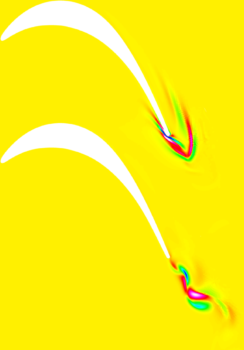
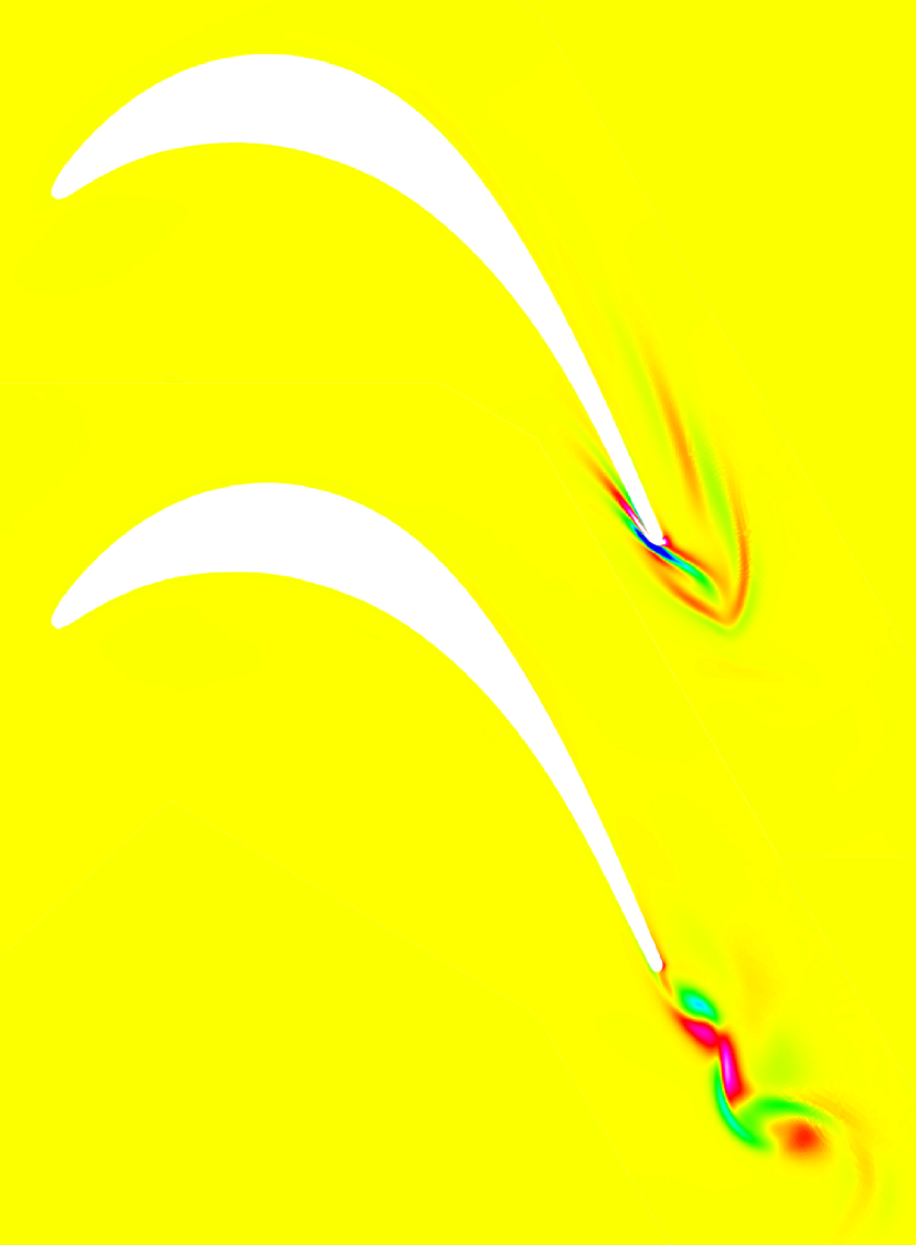
Figure 9: Normalised leading mode initial condition (left upper) and final state (left lower) at $L_{z}=1.95c$, for $\tau=T$, at zero initial phase, showing spanwise vorticity. The right-hand plot shows the same for the mode associated with the second singular value.

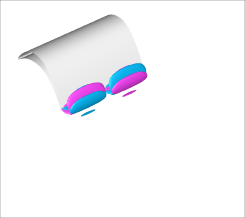
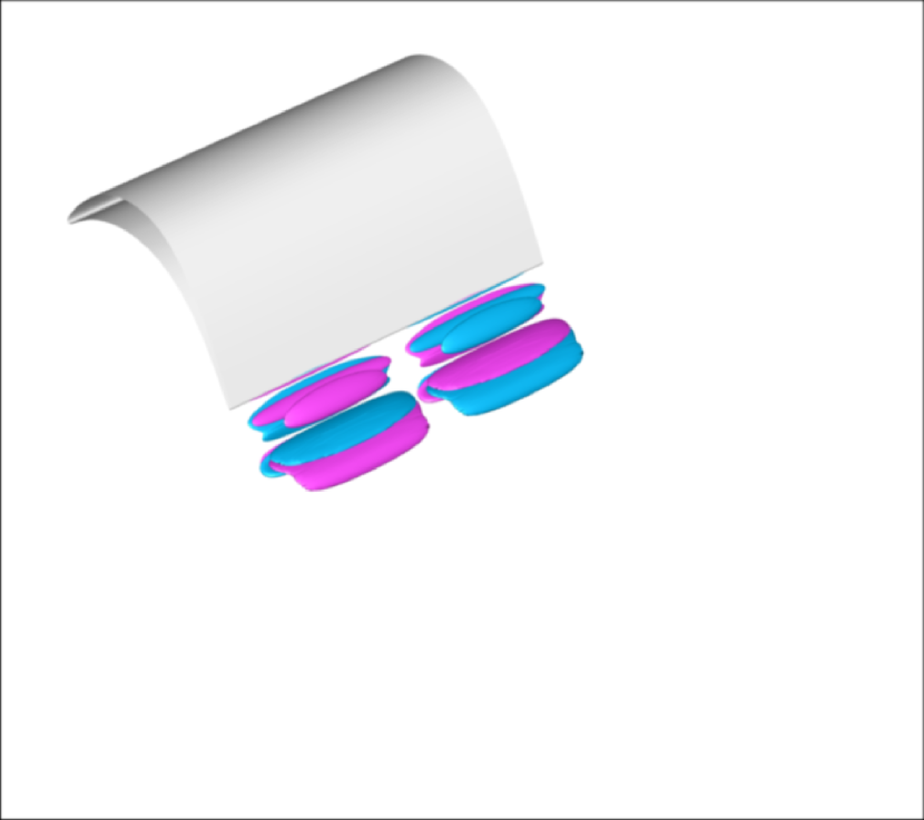
Figure 10: Normalised leading mode initial condition (left) and final state (right) at $L_{z}=1.95c$, for $\tau=T$, at zero initial phase. The mode has been combined with $10\times$ the base flow and the plots show iso-surfaces of streamwise vorticity at $\omega_{x}=\pm 0.6$

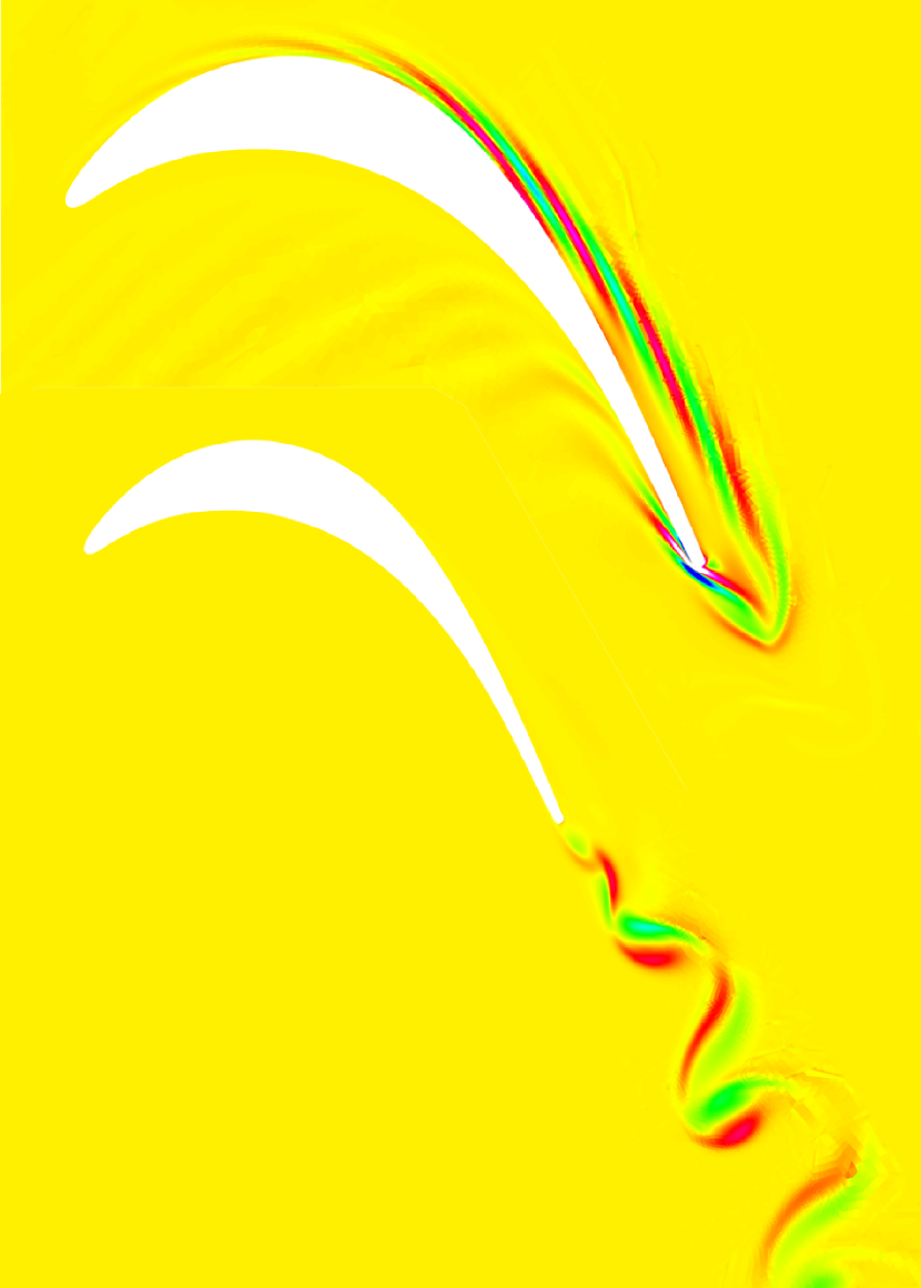
Figure 11: Normalised leading mode initial condition (upper) and final state (lower) at $\beta=0$ (2D case), for $\tau=8T$, at zero initial phase, showing spanwise vorticity

The preceding discussion has assumed an initial phase of $t_{0}=0$ (relating to the point in the shedding cycle) at $t=0$ as defined in figure 2. An investigation was also carried out to find the effects on the maximum attainable growth of varying this initial phase. At short growth horizons $\tau$, the growth achieved is only weakly dependent on $L_{z}$ and is achieved just before $t_{0}\sim 0.2$ as can be seen in figure 12. Furthermore the figure also shows the dependence on initial phase remains weak over a range of integration times $\tau$. We conclude from the figure that the dependence of growth on the initial phase $t_{0}$ is relatively unimportant.

\psfragscanon\psfrag{s01}[b][b]{\color[rgb]{0,0,0}\begin{tabular}[]{c}$\beta c$\end{tabular}}\psfrag{s02}[t][t]{\color[rgb]{0,0,0}\begin{tabular}[]{c}$t_{0}/T$\end{tabular}}\psfrag{s03}{\color[rgb]{0,0,0}\begin{tabular}[]{c}4.6\end{tabular}}\psfrag{s04}{\color[rgb]{0,0,0}\begin{tabular}[]{c}4.6\end{tabular}}\psfrag{s05}{\color[rgb]{0,0,0}\begin{tabular}[]{c}4.6\end{tabular}}\psfrag{s06}{\color[rgb]{0,0,0}\begin{tabular}[]{c}4.6\end{tabular}}\psfrag{s07}{\color[rgb]{0,0,0}\begin{tabular}[]{c}4.6\end{tabular}}\psfrag{s08}{\color[rgb]{0,0,0}\begin{tabular}[]{c}4.6\end{tabular}}\psfrag{s09}{\color[rgb]{0,0,0}\begin{tabular}[]{c}4.8\end{tabular}}\psfrag{s10}{\color[rgb]{0,0,0}\begin{tabular}[]{c}4.8\end{tabular}}\psfrag{s11}{\color[rgb]{0,0,0}\begin{tabular}[]{c}4.8\end{tabular}}\psfrag{s12}{\color[rgb]{0,0,0}\begin{tabular}[]{c}4.8\end{tabular}}\psfrag{s13}{\color[rgb]{0,0,0}\begin{tabular}[]{c}4.8\end{tabular}}\psfrag{s14}{\color[rgb]{0,0,0}\begin{tabular}[]{c}4.8\end{tabular}}\psfrag{s15}{\color[rgb]{0,0,0}\begin{tabular}[]{c}5\end{tabular}}\psfrag{s16}{\color[rgb]{0,0,0}\begin{tabular}[]{c}5\end{tabular}}\psfrag{s17}{\color[rgb]{0,0,0}\begin{tabular}[]{c}5\end{tabular}}\psfrag{s18}{\color[rgb]{0,0,0}\begin{tabular}[]{c}5.2\end{tabular}}\psfrag{s19}{\color[rgb]{0,0,0}\begin{tabular}[]{c}5.2\end{tabular}}\psfrag{s20}{\color[rgb]{0,0,0}\begin{tabular}[]{c}5.2\end{tabular}}\psfrag{s21}{\color[rgb]{0,0,0}\begin{tabular}[]{c}5.2\end{tabular}}\psfrag{s22}{\color[rgb]{0,0,0}\begin{tabular}[]{c}5.2\end{tabular}}\psfrag{s23}{\color[rgb]{0,0,0}\begin{tabular}[]{c}5.2\end{tabular}}\psfrag{s24}{\color[rgb]{0,0,0}\begin{tabular}[]{c}5.4\end{tabular}}\psfrag{s25}{\color[rgb]{0,0,0}\begin{tabular}[]{c}5.4\end{tabular}}\psfrag{s26}{\color[rgb]{0,0,0}\begin{tabular}[]{c}5.4\end{tabular}}\psfrag{s27}{\color[rgb]{0,0,0}\begin{tabular}[]{c}5.4\end{tabular}}\psfrag{s28}{\color[rgb]{0,0,0}\begin{tabular}[]{c}5.4\end{tabular}}\psfrag{s29}{\color[rgb]{0,0,0}\begin{tabular}[]{c}5.4\end{tabular}}\psfrag{x01}[t][t]{0}\psfrag{x02}[t][t]{0.2}\psfrag{x03}[t][t]{0.4}\psfrag{x04}[t][t]{0.6}\psfrag{x05}[t][t]{0.8}\psfrag{v01}[r][r]{0}\psfrag{v02}[r][r]{1}\psfrag{v03}[r][r]{2}\psfrag{v04}[r][r]{3}\psfrag{v05}[r][r]{4}\includegraphics{beta_t0_T00.25.eps}

\psfragscanon\psfrag{s01}[b][b]{\color[rgb]{0,0,0}\begin{tabular}[]{c}$\tau/T$\end{tabular}}\psfrag{s02}[t][t]{\color[rgb]{0,0,0}\begin{tabular}[]{c}$t_{0}/T$\end{tabular}}\psfrag{s03}{\color[rgb]{0,0,0}\begin{tabular}[]{c}1\end{tabular}}\psfrag{s04}{\color[rgb]{0,0,0}\begin{tabular}[]{c}1\end{tabular}}\psfrag{s05}{\color[rgb]{0,0,0}\begin{tabular}[]{c}1\end{tabular}}\psfrag{s06}{\color[rgb]{0,0,0}\begin{tabular}[]{c}1\end{tabular}}\psfrag{s07}{\color[rgb]{0,0,0}\begin{tabular}[]{c}1.5\end{tabular}}\psfrag{s08}{\color[rgb]{0,0,0}\begin{tabular}[]{c}1.5\end{tabular}}\psfrag{s09}{\color[rgb]{0,0,0}\begin{tabular}[]{c}1.5\end{tabular}}\psfrag{s10}{\color[rgb]{0,0,0}\begin{tabular}[]{c}2\end{tabular}}\psfrag{s11}{\color[rgb]{0,0,0}\begin{tabular}[]{c}2\end{tabular}}\psfrag{s12}{\color[rgb]{0,0,0}\begin{tabular}[]{c}2\end{tabular}}\psfrag{s13}{\color[rgb]{0,0,0}\begin{tabular}[]{c}2\end{tabular}}\psfrag{s14}{\color[rgb]{0,0,0}\begin{tabular}[]{c}2.5\end{tabular}}\psfrag{s15}{\color[rgb]{0,0,0}\begin{tabular}[]{c}2.5\end{tabular}}\psfrag{s16}{\color[rgb]{0,0,0}\begin{tabular}[]{c}2.5\end{tabular}}\psfrag{s17}{\color[rgb]{0,0,0}\begin{tabular}[]{c}3\end{tabular}}\psfrag{s18}{\color[rgb]{0,0,0}\begin{tabular}[]{c}3\end{tabular}}\psfrag{s19}{\color[rgb]{0,0,0}\begin{tabular}[]{c}3\end{tabular}}\psfrag{s20}{\color[rgb]{0,0,0}\begin{tabular}[]{c}3\end{tabular}}\psfrag{s21}{\color[rgb]{0,0,0}\begin{tabular}[]{c}3.5\end{tabular}}\psfrag{s22}{\color[rgb]{0,0,0}\begin{tabular}[]{c}3.5\end{tabular}}\psfrag{s23}{\color[rgb]{0,0,0}\begin{tabular}[]{c}3.5\end{tabular}}\psfrag{x01}[t][t]{0}\psfrag{x02}[t][t]{0.2}\psfrag{x03}[t][t]{0.4}\psfrag{x04}[t][t]{0.6}\psfrag{x05}[t][t]{0.8}\psfrag{v01}[r][r]{1}\psfrag{v02}[r][r]{2}\psfrag{v03}[r][r]{3}\psfrag{v04}[r][r]{4}\psfrag{v05}[r][r]{5}\includegraphics{t0_T_beta0.eps}

Figure 12: (left) $G_{\tau}$ with varying $t_{0}$ and $\beta$, $\tau=0.25T$; (right) $log_{10}(G(\tau))$ with varying $\tau$ and $t_{0}$, $\beta=0$

The relevant previous study Abdessemed09-1 demonstrated that although subharmonic effects were small, they were sufficient to induce asynchronous shedding and prevented the flow from going unstable. For the present problem we do not consider the asymptotic or long-time behaviour of perturbations but their behaviour over a shorter time horizon.

Results for the double-bladed mesh were tested for times up to eight shedding periods and agree well with the single blade situation. At these longer times, consideration of the least stable eigenmode would be more suitable. This leads to the conclusion that subharmonic effects are relatively unimportant in the transient growth problem and the assumed periodic boundary condition is a valid means to reduce the computational domain for the problem under study.

4 Discussion and conclusion

The transient behaviour of perturbations to linearised flow past a periodic array of T-106/300 low pressure turbine fan blade was investigated. The analysis was carried out at a Reynolds number of 2000 associated with periodic vortex shedding, used as a periodic base flow.

It is known from asymptotic analysis Abdessemed09-1 , the flow past an array of these turbine blades is marginally stable. The current analysis shows that long wavelength optimal perturbations associated with long time integration periods convect far downstream and eventually align with the asymtotically least stable eigenmode. The discovery of converging optimum growth for long integration times confirms the lack of a strong asymptotic instability.

It is found that the long-wavelength perturbations tend toward a purely two-dimensional case and that these perturbations are associated to maximum optimum growth in the asymptotic case approached by long time-integration. However, as we already know from two-dimensional DNS, the two-dimensional baseflow is stable for nonlinear flows and therefore also stable in a linear sense. It therefore may be assumed that the identified optimum growth associated to long wavelength perturbations is less significant than perturbations that are limited in spanwise wavelength. When considering short integration times it is indeed found that short-wavelength perturbations are of higher significance.

Short integration times have maximum optimal growth at shorter spanwise wavelengths and convect only a short distance downstream, exciting the near wake. We might hypothesise that in the presence of the neglected nonlinearity, the associated optimum modes cause shear layer separation, triggering wake instability. This would have to be demonstrated in a full nonlinear DNS. Furthermore, the spanwise length of a real LPT blade is naturally limited, giving an additional reason why short wavelength perturbation are more important than long wavelength disturbances of theoretical spanwise extent.

Our results are consistent with the understanding that transient growth mechanisms are associated with shear in the base flow feeding the perturbation energy growth. The results presented are consistent therefore with the cylinder results reported in the literature (both on transient growth mechanisms Abdessemed09 ; shabshth06 and on receptivity via the adjoint Luchini07 ) and with the previous work on the LPT fan blade used in this study Abdessemed09-1 .

It is hoped that the understanding developed will prove useful in controlling laminar boundary layer separation with a view to improving performance. For instance, the spatially periodic pattern in the shear layer can be quantified in the time-domain indicating disturbance frequencies susceptible to optimum amplification.

- (1) Abdessemed, N., Sharma, A.S., Sherwin, S.J., Theofilis, V.: Transient growth analysis of the flow past a circular cylinder. Phys. Fluids 21(4) (2009)
- (2) Abdessemed, N., Sherwin, S., Theofilis, V.: On unstable 2d basic states in low pressure turbine flows at moderate reynolds numbers. AIAA Paper 2004-2541 (2004)
- (3) Abdessemed, N., Sherwin, S., Theofilis, V.: Linear stability of the flow past a low pressure turbine blade. AIAA Paper 2006-3530 (2006)
- (4) Abdessemed, N., Sherwin, S.J., Theofilis, V.: Linear instability analysis of low pressure turbine flows. J. Fluid Mech. In press (2009)
- (5) Barkley, D., Blackburn, H.M., Sherwin, S.J.: Direct optimal growth analysis for timesteppers. Intnl J. Num. Meth. Fluids 57, 1435 (2008)
- (6) Barkley, D., Gomes, M.G.M., Henderson, R.D.: Three-dimensional instability in flow over a backward-facing step. J. Fluid Mech. 473, 167–190 (2002)
- (7) Barkley, D., Henderson, R.: Three-dimensional floquet stability analysis of the wake of a circular cylinder. J. Fluid Mech. 322, 215 – 241 (1996)
- (8) Blackburn, H., Sherwin, S.J., Barkley, D.: Convective instability and transient growth in steady and pulsatile stenotic flows. J. Fluid Mech. 607, 267–277 (2008)
- (9) Blackburn, H.M.: Three-dimensional instability and state selection in an oscillatory axisymmetric swirling flow. Phys. Fluids 14(11), 3983–3996 (2002)
- (10) Blackburn, H.M., Barkley, D., Sherwin, S.J.: Convective instability and transient growth in flow over a backward-facing step. J. Fluid Mech. 603, 271–304 (2008)
- (11) Blackburn, H.M., Lopez, J.M.: The onset of three-dimensional standing and modulated travelling waves in a periodically driven cavity flow. J. Fluid Mech. 497, 289–317 (2003)
- (12) Blackburn, H.M., Sherwin, S.J.: Instability modes and transition of pulsatile stenotic flow: pulse-period dependence. J. Fluid Mech. 573, 57–88 (2007)
- (13) Butler, K.M., Farrell, B.F.: Three-dimensional optimal perturbations in viscous shear flow. Physics of Fluids A: Fluid Dynamics 4, issue 8, 1637–1650 (1992)
- (14) Corbett, P., Bottaro, A.: Optimal perturbations for boundary layers subject to stream-wise pressure gradient. Phys. Fluids 12(1), 120–130 (2000)
- (15) Ding, Y., Kawahara, M.: Linear stability of incompressible flow using a mixed finite element method. J. Comput. Phys. 139, 243–273 (1998)
- (16) Drazin, P., Reid, W.: Hydrodynamic stability. Cambridge University Press (1981)
- (17) Ehrenstein, U.: On the linear stability of channel flows over riblets. Phys. Fluids 8, 3194–3196 (1996)
- (18) Ehrenstein, U., Gallaire, F.: On two-dimensional temporal modes in spatially evolving open flows: the flat-plate boundary layer. J. Fluid Mech. 536, 209–218 (2005)
- (19) Elston, J.R., Blackburn, H.M., Sheridan, J.: The primary and secondary instabilities of flow generated by an oscillating circular cylinder. J. Fluid Mech. 550, 359–389 (2006)
- (20) Farrell, B.F.: Optimal excitation of perturbations in viscous shear flow. Phys. Fluids 31(8), 2093–2102 (1988)
- (21) Giannetti, F., Luchini, P.: Structural receptivity of the first instability of the cylinder wake. J. Fluid Mech. 581, 167–197 (2007)
- (22) González, L., Theofilis, V., Gómez-Blanco, R.: Finite element methods for viscous incompressible biglobal instability analysis on unstructured meshes. AIAA J. 45(4), 840–854 (2007)
- (23) Henderson, R., Barkley, D.: Secondary instability in the wake of a circular cylinder. Phys. Fluids 6, No. 8, 1683 – 1685 (1996)
- (24) Hœpffner, J., Brandt, L., Henningson, D.S.: Transient growth on boundary layer streaks. J. Fluid Mech. 537, 91–100 (2005)
- (25) J. L. Guermond, J.S.: A new class of truly consistent splitting schemes for incompressible flows. Journal of Computational Physics 192 (1), 262–276 (2003)
- (26) Karniadakis, G., Israeli, M., Orszag, S.: High-order splitting methods for the incompressible Navier-Stokes equations. Journal of Computational Physics 97, 414–443 (1991)
- (27) Karniadakis, G.E., Sherwin, S.J.: Spectral/ element methods for CFD. OUP (1999)
- (28) Luchini, P.: Reynolds-number-independent instability of the boundary layer over a flat surface: optimal perturbations. J. Fluid Mech. 404, 289–309 (2000)
- (29) Marquet, O., Sipp, D., Jacquin, L.: Global optimal perturbations in a separated flow over a backward-rounded-step. In: 36th AIAA Fluid Dyn. Conf. and Exhibit. San Francisco (2006). Paper no. 2006-2879
- (30) Schatz, M., Barkley, D., Swinney, H.: Instabilities in spatially periodic channel flow. Phys. Fluids 7, 344–358 (1995)
- (31) Schmid, P., Henningson, D.: Stability and transition in shear flows. Springer (2001)
- (32) Schmid, P.J.: Nonmodal stability theory. Ann. Rev. Fluid Mech. (39), 129–162 (2007)
- (33) Sharma, A., Abdessemed, N., Sherwin, S., Theofilis, V.: Optimal growth modes of flows in complex geometries. In: IUTAM Symposium on Flow Control and MEMS, London, UK (2006)
- (34) Sherwin, S.J., Blackburn, H.M.: Three-dimensional instabilities and transition of steady and pulsatile flows in an axisymmetric stenotic tube. J. Fluid Mech. 533, 297–327 (2005)
- (35) Theofilis, V.: Advances in global linear instability of nonparallel and three-dimensional flows. Prog. Aero. Sciences 39 (4), 249–315 (2003)
- (36) Theofilis, V., Duck, P.W., Owen, J.: Viscous linear stability analysis of rectangular duct and cavity flows. J. Fluid Mech. 505, 249–286 (2004)
- (37) Theofilis, V., Fedorov, A., Obrist, D., Dallmann, U.C.: The extended Görtler-Hämmerlin model for linear instability of three-dimensional incompressible swept attachment-line boundary layer flow. J. Fluid Mech. 487, 271–313 (2003)
- (38) Theofilis, V., Hein, S., Dallmann, U.: On the origins of unsteadiness and three-dimensionality in a laminar separation bubble. Phil. Trans. Roy. Soc. London (A) 358, 3229–3246 (2000)
- (39) Trefethen, L.N., Trefethen, A.E., Reddy, S.C., Driscoll, T.: Hydrodynamic stability without eigenvalues. Science 261, 578–584 (1993)
- (40) Tuckerman, L., Barkley, D.: Bifurcation analysis for timesteppers. In: E. Doedel, L. Tuckerman (eds.) Numerical Methods for Bifurcation Problems and Large-Scale Dynamical Systems, vol. 119, pp. 543–466. Springer, New York (2000)