Population genetics of neutral mutations in exponentially growing cancer cell populations

Abstract

In order to analyze data from cancer genome sequencing projects, we need to be able to distinguish causative, or “driver,” mutations from “passenger” mutations that have no selective effect. Toward this end, we prove results concerning the frequency of neutural mutations in exponentially growing multitype branching processes that have been widely used in cancer modeling. Our results yield a simple new population genetics result for the site frequency spectrum of a sample from an exponentially growing population.

t1Supported by NSF Grant DMS-10-05470 from the probability program and NIH Grant R01-GM096190-02.

1 Introduction

It is widely accepted that cancers result from an accumulation of mutations that increase the fitness of tumor cells compared to the cells that surround them. A number of studies [Sjöblom et al. (2006), Wood et al. (2007), Parsons et al. (2008), The Cancer Genome Atlas (2008) and Jones et al. (2008, 2010)] have sequenced the genomes of tumors in order to find the causative or “driver” mutations. However, due to the large number of genes being sequenced, one also finds a large number of “passenger” mutations that are genetically neutral and hence have no role in the disease.

Table 1: Colorectal cancer data from Wood et al. (2007)

	NS mutations		Passenger probability
Gene	Discovery	Validation	External	SNP	NS/S
APC	$171$	$138$	0.00	0.00	0.00
KRAS	$79$	$62$	0.00	0.00	0.00
TP53	$79$	$61$	0.00	0.00	0.00
PIK3CA	$28$	$23$	0.00	0.00	0.00
FBXW7	$14$	$9$	0.00	0.00	0.00
EPHA3	$10$	$6$	0.00	0.00	0.00
TCF7L2	$10$	$7$	0.00	0.00	0.01
ADAMTSL3	$9$	$5$	0.00	0.00	0.03
NAV3	$8$	$3$	0.00	0.01	0.64
GUCY1A2	$7$	$4$	0.00	0.00	0.01
MAP2K7	$6$	$3$	0.00	0.00	0.02
PRKD1	$5$	$3$	0.00	0.00	0.39
MMP2	$5$	$2$	0.00	0.02	0.61
SEC8L1	$5$	$2$	0.00	0.03	0.63
GNAS	$5$	$2$	0.00	0.04	0.67
ADAMTS18	$5$	$2$	0.00	0.07	0.82
RET	$5$	$2$	0.01	0.17	0.89
TNN	$5$	$0$	0.00	0.11	0.81

To explain the issues involved in distinguishing the two types of mutations, it is useful to take a look at a data set. Wood et al. (2007) did a “discovery” screen in which 18,191 genes were sequenced in 11 colorectal cancers, and then a “validation” screen in which the top candidates were sequenced in 96 additional tumors. The 18 genes that were mutated five or more times mutated in the discovery screen are given in Table 1. Here NS is short for nonsynonymous mutation, a nucleotide substitution that changes the amino acid in the corresponding protein. The top four genes in the list are well known to be associated with cancer.

• Adenomatous polyposis coli (APC) is a tumor suppressor gene. That is, when both copies of the gene are knocked out in a cell, uncontrolled growth results. It is widely accepted that the first stages of colon cancer are the loss of both copies of the APC gene from some cell, see, e.g., Figure 4 in Luebeck and Moolgavkar (2002).

• Kras is an oncogene, i.e., one which causes trouble when a mutation increases its expression level. Once Kras is turned on it recruits and activates proteins necessary for the propagation of growth factors.

• TP53 which produces the protein $p53$ (named for its 53 kiloDalton size) is loved by those who study “complex networks,” since it is known to be important and appears with very high degree in protein interaction networks. $p53$ regulates the cell cycle and has been called the “master watchman” referring to its role in conserving stability by preventing genome mutation.

• The protein kinase PIK3CA is not as famous as the other three genes (e.g., it does not yet have its own Wikipedia page) but it is known to be associated with breast cancer. In a study of eight ovarian cancer tumors in Jones et al. (2010), an $A\to G$ mutation was found at base 180,434,779 on chromosome 3 in six tumors.

The next three genes on the list with the unromantic names FBXW7, EPHA3, and TCF7L2 are all either known to be implicated in cancer or are likely suspects because of the genetic pathways they are involved in. Use google if you want to learn more about them.

The methodology that Wood et al. (2007) used for assessing passenger probabilities is explained in detail in Parmigiani et al. (2007). In principle this is straightforward: one calculates the probability that the observed number of mutations would be seen if all mutations were neutral. The first problem is to estimate the neutral mutation rate. In the column labeled “external” this estimate comes from experimentally observed rates, while in the column labeled “SNP” they used the mutations observed in the study, with the genes declared to be under selection excluded. The estimation problem is made more complicated by the fact that DNA mutation rates are context dependent. The two nucleotides in what geneticists call a CpG (the p refers to the phosphodiester bond between the adjacent cytosine and the guanine nucleotides) each mutate at roughly 10 times the rate of a thymine.

The third method for estimating passenger probabilities, inspired by population genetics, is to look at the ratio of nonsynonymous to synonymous mutations after these numbers have been scaled by dividing by the number of opportunities for the two types of mutations. While the top dozen genes show strong signals of not being neutral, as one moves down the list the situation becomes less clear, and the probabilities reported in the last three columns sometimes give conflicting messages. The passenger probabilities in the last column are in most cases higher and in some cases such as NAV3 and tthe last three genes in the table are radically different. My personal feeling is that in this context the NS/S test does not have enough mutations to give it power to detect selection, but perhaps it is the other two methods that are being fooled.

To investigate the number and frequency of neutral mutations observed in cancer sequencing studies, we will use a well-studied framework in which an exponentially growing cancer cell population is modeled as a multi-type branching process. Cells of type $i\geq 0$ give birth at rate $a_{i}$ and die at rate $b_{i}$, where the growth rate $\lambda_{i}=a_{i}-b_{i}>0$. Thinking of cancer we will restrict our attention to the case in which $i\to\lambda_{i}$ is increasing. To take care of mutations, we suppose that individuals of type $i$ also give birth at rate $u_{i+1}$ to individuals of type $i+1$ that have one more mutation. This is slightly different from the approach of having mutations with probability $u_{i+1}$ at birth, which translates into a mutation rate of $a_{i}u_{i+1}$, and this must be kept in mind when comparing with other results.

Let $\tau_{k}$ be the time of the first type $k$ mutation and let $\sigma_{k}$ be the time of the first type $k$ mutation that gives rise to a family that lives forever. Following up on initial studies by Iwasa, Nowak and Michor (2006), and Haeno, Iwasa and Michor (2007), Durrett and Moseley (2010) have obtained results for $\tau_{k}$ and limit theorems for the growth of $Z_{k}(t)$, the number of type $k$’s at time $t$. These authors did not consider $\sigma_{k}$, but the extension is trivial: each type $k$ mutation gives rise to a family that lives forever with probability $\lambda_{k}/a_{k}$, so all we have to do is to replace $u_{k}$ in the limit theorem for $\tau_{k}$ by $u_{k}\lambda_{k}/a_{k}$.

1.1 Wave 0 results

To begin to understand the behavior of neutral mutations in our cancer model, we first consider those that occur to type 0’s, which are a branching process $Z_{0}(t)$ in which individuals give birth at rate $a_{0}$ and die at rate $b_{0}<a_{0}$. It is well-known, see O’Connell (1993), that if we condition $Z_{0}(t)$ to not die out, and let $Y_{0}(t)$ be the number of individuals at time $t$ whose families do not die out, then $Y_{0}(t)$ is a Yule process in which births occur at rate $\gamma=\lambda_{0}/a_{0}$. Our first problem is to investigate the population site frequency spectrum,

$$F(x)=\lim_{t\to\infty}F_{t}(x),$$ (1)

where $F_{t}(x)$ is the expected number of neutral “passenger” mutations present in more than a fraction $x$ of the individuals at time $t$. To begin to compute $F(x)$, we note that

$$Y_{0}(t)/Z_{0}(t)\to\gamma\qquad\mbox{in probability,}$$ (2)

since each of the $Z_{0}(t)$ individuals at time $t$ has a probability $\gamma$ of starting a family that does not die out, and the events are independent for different individuals.

It follows from (2) that it is enough to investigate the frequencies of neutral mutations within $Y_{0}$. If we take the viewpoint of the infinite alleles model, where each mutation is to a type not seen before, then results can be obtained from Durrett and Schweinsberg’s (2005) study of a gene duplication model. In their system there is initially a single individual of type 1. No individual dies and each individual independently gives birth to a new individual at rate 1. When a new individual is born it has the same type as its parent with probability $1-r$ and with probability $r$ is a new type which is different from all previously observed types.

Let $T_{N}$ be the first time there are $N$ individuals and let $F_{S,N}$ be the number of families of size $>S$ at time $T_{N}$. Omitting the precise error bounds given in Theorem 1.3 of Durrett and Schweinsberg (2005), that result says

$$F_{S,N}\approx r\Gamma\biggl{(}\frac{2-r}{1-r}\biggr{)}NS^{-1/(1-r)}\qquad\mbox{for $1\ll S\ll N^{1-r}$}.$$ (3)

The upper cutoff on $S$ is needed for the result to hold. When $S\gg N^{1-r}$, $EF_{S,N}$ decays exponentially fast.

As mentioned above, the last conclusion gives a result for a branching process with mutations according to the infinite alleles model, a subject first investigated by Griffiths and Pakes (1988). To study DNA sequence data, we are more interested in the frequencies of individual mutations. Using ideas from Durrett and Schweinsberg (2004) it is easy to show:

Theorem 1

If passenger mutations occur at rate $\nu$ then $F(x)=\nu/\gamma x$.

This theorem describes the population site frequency spectrum. As in Section 1.5 of Durrett (2008), this can be used to derive the site frequency spectrum for a sample of size $n$. Let $\eta_{n,m}$ be the number of sites in a sample of size $n$ where $m$ individuals in the sample have the mutant nucleotide. If one considers the Moran model in a population of constant size $N$ then

$$E\eta_{n,m}=\frac{2N\nu}{m}\qquad\mbox{for $1\leq m<n$.}$$ (4)

Using Theorem 1 now, we get a new result concerning the population genetics of exponentially growing populations. Here we are considering a Moran model in an exponentially growing population, see, e.g., Section 4.2 of Durrett (2008), rather than a branching process.

Theorem 2

Suppose that the mutation rate is $\nu$ and the population size $t$ units before the present is $N(t)=Ne^{-\gamma t}$ then as $N\to\infty$

$$E\eta_{n,m}\cases{\displaystyle\to\frac{n\nu}{\gamma}\cdot\frac{1}{m(m-1)},&\quad$2\leq m<n,$\vspace*{2pt}\cr\displaystyle\sim\frac{n\nu}{\gamma}\cdot\log(N\gamma),&\quad$m=1,$}$$ (5)

where $a_{N}\sim b_{N}$ means $a_{N}/b_{N}\to 1$.

To explain the result for $m=1$, we note that, as Slatkin and Hudson (1991) observed, genealogies in exponentially growing population tend to be star-shaped. The time required for $Y_{0}(t)$ to reach size $N\gamma$ (and hence roughly the time for $Z_{0}(t)$ to reach size $N$) is $\sim(1/\gamma)\log(N\gamma)$, so the number of mutations on our $n$ lineages is roughly $n\nu$ times this. Note that, (i) for a fixed sample size, $E\eta_{n,m}$, $2\leq m<n$ are bounded independent of the final population size, and (ii) in contrast to (4), the sample size replaces the population size in formula (5).

The result in Theorem 2 is considerably simpler than previous formulas. Let $L(t)$ be the number of lineages $t$ units of time before the present. For $2\leq k\leq n$ let $T_{k}=\sup\{t\dvtx L(t)\geq k\}$ be the first time at which the number of lineages is reduced to $k-1$, and let $S_{k}=T_{k}-T_{k+1}$ where $T_{n+1}=0$. Griffiths and Tavaré (1998) have shown that under some mild assumptions (coalescent times have continuous distributions, only two lineages coalesce at once, all coalescence events have equal probability, Poisson process of mutations) the probability that a segregating site has $b$ mutant bases is

$$q_{n,b}=\frac{(n-b-1)!(b-1)!\sum_{k=2}^{n}k(k-1){{n-k}\choose{b-1}}ES_{k}}{(n-1)!\sum_{k=2}^{n}kES_{k}}.$$ (6)

To apply this result to the coalescent with population size $N(t)=Ne^{-\gamma t}$, one needs formulas for $ES_{k}$. See for example (52) in Polanski, Bobrowski, and Kimmel (2003). However, these formulas are complicated and difficult to evaluate numerically, since they involve large terms of alternating size. To connect (6) with the result in Theorem 2, we write

$$q_{n,1}=1-\frac{\sum_{k=2}^{n-1}k(n-k)ES_{k}}{(n-1)\sum_{k=2}^{n}kES_{k}}.$$

Equation (3) below will show that $ES_{n}\sim\log N$ while for $2\leq k<n$, $ES_{k}=O(1)$ so we have $1-q_{n,1}=O(1/\log N)$ in agreement with (5).

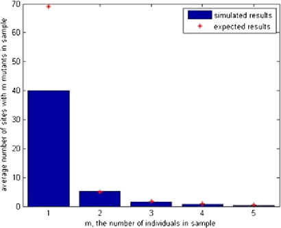
Figure 1: Simulated site frequency spectrum when $\nu=\gamma$, sample size $n=10$, and population size $N=100\mbox{,}000$.

To check (5) Yifei Chen, a participant in a summer REU associated with Duke’s math biology Research Training Grant, performed simulations. Figure 1 gives results for the average of 100 simulations with the indicated parameters. The agreement is almost perfect for $m\geq 2$ but the formula considerably over estimates the number of singletons with (5), predicting 69.07 versus an observed value of about 40. Given the approximations used in the proof of Theorem 2 in Section 2 for the case $m=1$, this is not surprising. The next result derives a much better result for $E\eta_{n,1}$ which gives a value of 36.66. See (27) for details of the numerical calculation.

Theorem 3

$$E\eta_{n,1}\approx\frac{\nu}{\gamma}\sum_{k=1}^{N\gamma}\frac{n}{n+k}\cdot\frac{k}{n+k-1}.$$

Here $\approx$ means simply that this is an approximation which is better for finite $N$. As $N\to\infty$ the right-hand side $\sim(n\nu/\gamma)\log(N\gamma)$ the answer in Theorem 2.

The results for $E\eta_{n,m}$ are useful for population genetics, but are not really relevant to cancer modeling. To investigate genetic diversity in the exponentially growing population of humans, you would sequence the DNA of a sample of individuals from the population. However, in the study of cancer each patient has their own exponentially growing cell population, so it is more interesting to have the information provided by Theorem 1 about the fraction of cells in the population with a given mutation.

To illustrate the use of Theorem 1 suppose $\gamma=\lambda_{0}/a_{0}=0.01$ and $\nu=10^{-5}$. In support of the numbers we note that Bozic et al. (2010) estimate that the selective advantage provided by a typical cancer driver mutation is $0.004\pm 0.0004$. As for the second, if the per nucleotide mutation rate is $10^{-8}$ and there are 1000 nucleotides in a gene then a mutation rate of $10^{-5}$ per gene results. In this case Theorem 1 predicts if we focus only on one gene then the expected number of mutations with frequency $>0.1$ is

$$F(0.1)=10^{-5+2+1}=0.01$$ (7)

so, to a good first approximation, no particular neutral mutation occurs with an appreciable frequency. Of course, if we are sequencing 20,000 genes then there will be a few hundred passenger mutations seen in a given individual. On the other hand there will be very few specific neutral mutations that will appear multiple times in the sample.

1.2 Wave 1 results

We refer to the collection of type $k$ individuals as wave $k$. In order to analyze the cancer data, we also need results for neutral mutations in waves $k>0$ of the multitype branching process. We begin by recalling results from Durrett and Moseley (2010) for type 1 individuals in the process with $Z_{0}(0)=1$ when we condition the event $\Omega^{0}_{\infty}$ that the type 0’s do not die out. Let $\sigma_{1}$ be the time of the first “successful” type 1 mutation that gives rise to family that does not die out. Then $\sigma_{1}$ has median

$$s^{1}_{1/2}=\frac{1}{\lambda_{0}}\log\biggl{(}\frac{\lambda_{0}^{2}a_{1}}{a_{0}u_{1}\lambda_{1}}\biggr{)}$$ (8)

and as $u_{1}\to 0$

$$P(\sigma_{1}>s^{1}_{1/2}+x/\lambda_{0})\to(1+e^{x})^{-1}.$$ (9)

For (8) see (7) in Durrett and Moseley (2010) and drop the $1$ inside the logarithm. The second result follows from the reasoning for (6) there.

In investigating the growth of type 1’s, it is convenient mathematically to assume that $Z^{*}_{0}(t)=V_{0}e^{\lambda_{0}t}$ for $t\in(-\infty,\infty)$ and to let $Z_{k}^{*}(t)$ be the number of type $k$’s at time $t$ in this system. Here the star is to remind us that we have extended $Z_{0}$ to negative times. The probability of a mutation to type 1 at times $t\leq 0$ is $\leq V_{0}u_{1}/\lambda_{0}$. In the concrete example $u_{1}/\lambda_{0}=10^{-3}$, so this is likely to have no effect. The last calculation omits two details that almost cancel out. When we condition on survival of the type 0’s, $EV_{0}=a_{0}/\lambda_{0}$, but the probability a type 1 mutation survives for all time is $\lambda_{1}/a_{1}$. Since $a_{0}\approx a_{1}$ we are too low by a factor of $\lambda_{1}/\lambda_{0}=2$.

Durrett and Moseley (2010) have shown:

Theorem 4

If we regard $V_{0}$ as a fixed constant then as $t\to\infty$, $e^{-\lambda_{1}t}\times Z_{1}^{*}(t)\to V_{1}$ where $V_{1}$ is the sum of the points in a Poisson process with mean measure $\mu(x,\infty)=c_{\mu,1}u_{1}V_{0}x^{-\alpha}$ with $\alpha=\lambda_{0}/\lambda_{1}$ and

$$c_{\mu,1}=\frac{1}{a_{1}}\biggl{(}\frac{a_{1}}{\lambda_{1}}\biggr{)}^{\alpha}\Gamma(\alpha).$$ (10)

The Laplace transform $E(e^{-\theta V_{1}}|V_{0})=\exp(-c_{h,1}u_{1}V_{0}\theta^{\alpha})$ where $c_{h,1}=\break c_{\mu,1}\Gamma(1-\alpha)$. If $V_{0}$ is $\operatorname{exponential}(\lambda_{0}/a_{0})$ then

$$E\exp(-\theta V_{1})=\bigl{(}1+c_{h,1}u_{1}(a_{0}/\lambda_{0})\theta^{\alpha}\bigr{)}^{-1}.$$ (11)

Here, and in what follows, constants like $c_{\mu,1}$, $c_{h,1}$, and $c_{\theta,1}$ will depend on the branching process parameters $a_{i}$ and $b_{i}$, but not on the mutation rates $u_{i}$. The constant here is equal to, but written differently from, the one in Durrett and Moseley

$$c_{h,1}=\frac{1}{\lambda_{0}}\biggl{(}\frac{a_{1}}{\lambda_{1}}\biggr{)}^{\alpha-1}\Gamma(1+\alpha)\Gamma(1-\alpha)=\frac{1}{a_{1}}\frac{\lambda_{1}}{\lambda_{0}}\biggl{(}\frac{a_{1}}{\lambda_{1}}\biggr{)}^{\alpha}\alpha\Gamma(\alpha)\Gamma(1-\alpha).$$

To prepare for later results note that the formula for the Laplace transform shows that conditional on $V_{0}$, $V_{1}$ has a one sided stable distribution with index $\alpha$.

The point process in Theorem 4 describes the contributions of the successful type 1 mutations to $Z_{1}(t)$. The first such mutation occurs at time $\sigma_{1}$, which has median $s^{1}_{1/2}$. The derivation of Theorem 4 is based on the observation that a mutation at time $s$ will grow to size $\approx e^{\lambda_{1}(t-s)}W_{1}$ by time $t$, where $W_{1}$ has distribution

$$W_{1}=_{d}\frac{b_{1}}{a_{1}}\delta_{0}+\frac{\lambda_{1}}{a_{1}}\operatorname{exponential}(\lambda_{1}/a_{1})$$

and hence make a contribution of $e^{-\lambda_{1}(s-s^{1}_{1/2})}$ to the limit $\bar{V}_{1}$. Thus we expect that most of the mutations that make a significant contribution will come within a time $O(1/\lambda_{1})$ of $s^{1}_{1/2}$.

The complicated constants in Theorem 4 can be simplified if we instead look at the limit

$$e^{-\lambda_{1}(t-s^{1}_{1/2})}Z_{1}^{*}(t)\to\bar{V}_{1}=_{d}V_{1}\exp(\lambda_{1}s^{1}_{1/2}).$$

Using the definition of $s^{1}_{1/2}$ in (8) and recalling $\alpha=\lambda_{0}/\lambda_{1}$ we see that

$$\exp(\lambda_{1}s^{1}_{1/2})=\biggl{(}\frac{\lambda_{0}a_{1}}{a_{0}u_{1}}\cdot\alpha\biggr{)}^{1/\alpha}$$

and hence using (11)

$$E\exp(-\theta\bar{V}_{1})=\biggl{(}1+\alpha\Gamma(\alpha)\Gamma(1-\alpha)\biggl{(}\frac{a_{1}\theta}{\lambda_{1}}\biggr{)}^{\alpha}\biggr{)}^{-1}.$$ (12)

The combination of Gamma functions is easy to evaluate, since Euler’s reflection function implies that

$$\alpha\Gamma(\alpha)\Gamma(1-\alpha)=\frac{\pi\alpha}{\sin(\pi\alpha)}>1.$$ (13)

A second look at (12) shows that $a_{1}\bar{V}_{1}/\lambda_{1}$ has a distribution that only depends on $\alpha$. For comparison, note that if $V_{0}$ is $\operatorname{exponential}(\lambda_{0}/a_{0})$ then $a_{0}V_{0}/\lambda_{0}$ is $\operatorname{exponential}(1)$.

Using results for one-sided stable laws, Durrett et al. (2011) were able to prove results about the genetic diversity of wave 1. Define Simpson’s index to be the limiting probability two randomly chosen individuals in wave 1 are descended from the same type 1 mutation. In symbols, it is the $p=2$ case of the following definition

$$R_{p}=\sum_{i=1}^{\infty}\frac{X_{i}^{p}}{V_{1}^{p}},$$

where $X_{1}>X_{2}>\cdots$ are points in the Poisson process and $V_{1}$ is the sum. The result for the mean, which comes from a result of Fuchs, Joffe and Teugels (2001), is much simpler than one could reasonably expect.

Theorem 5

$ER_{2}=1-\alpha$.

After this paper was written Jason Schweinsberg explained to me that the points $Y_{i}=X_{i}/V_{1}$ have the Poisson–Dirichlet distribution $\mathrm{PD}(\alpha,0)$, so Theorem 5 follows from (3.6) in Pitman (2006). For our purposes it is easier to refer to (6) in Pitman and Yor (1997) where it is shown that

$$E\sum_{i=1}^{\infty}f(Y_{i})=\frac{1}{\Gamma(\alpha)\Gamma(1-\alpha)}\int_{0}^{1}f(u)u^{-\alpha-1}(1-u)^{\alpha-1}.$$

Taking $f(x)=x^{p}$ we find that $R_{p}=\sum_{i}X_{i}^{p}/V_{k}^{p}$ has

$$ER_{p}=E\sum_{i}Y_{i}^{p}=\frac{\Gamma(p-\alpha)}{\Gamma(1-\alpha)\Gamma(p)}.$$

Using formulas in Logan et al. (1973) one can derive results for the distribution of $R_{2}^{-1/2}$. Work of Darling (1952) leads to information about the distribution of the fraction in the largest clone $X_{1}/V_{1}$. In particular,

Theorem 6

$V_{1}/X_{1}$ has mean $1/(1-\alpha)$.

Since $1/x$ is convex, $E(X_{1}/V_{1})>1/E(V_{1}/X_{1})=1-\alpha$.

Theorems 5 and 6 suggest that if we are interested in understanding neutral mutations in say 90% of the population when wave 1 is dominant, then we can restrict our attention to the families generated by a small number of the most prolific type 1 mutants. (The number we need to consider will be large if $\alpha$ is close to 1.) The result in (7) suggests that we can ignore neutral mutations within the descendants of these type 1 mutations. Mutations that occur on the genealogies of the $i$th largest mutations will appear in all of their descendants and hence have frequency $X_{i}/V_{1}$. As remarked above (and explained in more detail in Section 3), the genealogies of the most prolific type 1 mutants will be approximately star-like so they will mostly have different mutations. Note that here, in contrast to the reasoning that led to (21) there are several individuals founding different subpopulations whose genealogies have collected neutral mutations.

1.3 Wave $k$ results

Once Theorem 4 was established it was straightforward to extend the result by induction. Let $\alpha_{k}=\lambda_{k-1}/\lambda_{k}$,

$$c_{\mu,k}=\frac{1}{a_{k}}\biggl{(}\frac{a_{k}}{\lambda_{k}}\biggr{)}^{\alpha_{k}}\Gamma(\alpha_{k})\quad\mbox{and}\quad c_{h,k}=c_{\mu,k}\Gamma(1-\alpha_{k}).$$ (14)

Let $c_{\theta,0}=a_{0}/\lambda_{0}$, $\mu_{0}=1$ and inductively define for $k\geq 1$

$$c_{\theta,k} = c_{\theta,k-1}c_{h,k}^{\lambda_{0}/\lambda_{k-1}},$$ (15)

$$\mu_{k} = \mu_{k-1}u_{k}^{\lambda_{0}/\lambda_{k-1}}=\prod_{j=1}^{k}u_{j}^{\lambda_{0}/\lambda_{j-1}}.$$ (16)

Durrett and Moseley (2010) have shown:

Theorem 7

Suppose $Z^{*}_{0}(t)=V_{0}e^{\lambda_{0}t}$ for $t\in(-\infty,\infty)$ where $V_{0}$ is$\operatorname{exponential}(\lambda_{0}/a_{0})$.

$$e^{-\lambda_{k}t}Z^{*}_{k}(t)\to V_{k}\qquad\mbox{a.s.}$$

Let $\mathcal{F}^{k-1}_{\infty}$ be the $\sigma$-field generated by $Z^{*}_{j}(t)$, $j\leq k-1$, $t\geq 0$. $(V_{k}|\mathcal{F}^{k-1}_{\infty})$ is the sum of the points in a Poisson process with mean measure $\mu(x,\infty)=c_{\mu,k}u_{k}V_{k-1}x^{-\alpha_{k}}$.

$$E(e^{-\theta V_{k}}|\mathcal{F}^{k-1}_{\infty})=\exp(-c_{h,k}u_{k}V_{k-1}\theta^{\lambda_{k-1}/\lambda_{k}})$$

and hence

$$Ee^{-\theta V_{k}}=(1+c_{\theta,k}\mu_{k}\theta^{\lambda_{0}/\lambda_{k}})^{-1}.$$ (17)

Using Theorem 7 it is easy to analyze $\tau_{k+1}$, the waiting time for the first type $k+1$. Details of the derivations of (18) and (19) are given in Section 4. The median of $\tau_{k+1}$ is

$$t^{k+1}_{1/2}=\frac{1}{\lambda_{0}}\log\biggl{(}\frac{\lambda_{k}^{\lambda_{0}/\lambda_{k}}}{c_{\theta,k}\mu_{k+1}}\biggr{)}=\frac{1}{\lambda_{k}}\log(\lambda_{k})-\frac{1}{\lambda_{0}}\log(c_{\theta,k}\mu_{k+1})$$ (18)

and as in the case of $\tau_{1}$

$$P(\tau_{k+1}>t^{k+1}_{1/2}+x/\lambda_{0})\approx(1+e^{x})^{-1}.$$

Again the result for the median $s^{k+1}_{1/2}$ of the time $\sigma_{k+1}$ of the first mutation to type $k+1$ with a family that does not die out can be found by replacing $u_{k+1}$ by $u_{k+1}\lambda_{k+1}/a_{k+1}$.

Formula (18), due to Durrett and Moseley (2010), is not very transparent due to the complicated constants. We will obtain a more intuitive result by looking at the difference $s^{k+1}_{1/2}-s^{k}_{1/2}$. After some algebra, hidden away in Section 4, we have

$$\qquad s^{k+1}_{1/2}-s^{k}_{1/2}=\frac{1}{\lambda_{k}}\log\biggl{(}\frac{\lambda^{2}_{k}a_{k+1}}{a_{k}u_{k+1}\lambda_{k+1}}\biggr{)}-\frac{1}{\lambda_{k-1}}\log\bigl{(}\alpha_{k}\Gamma(\alpha_{k})\Gamma(1-\alpha_{k})\bigr{)}.$$ (19)

Neutral mutations. Returning to our main topic, it follows from the first conclusion in Theorem 7 that the results of Theorems 5 and 6 hold for wave $k$ when $\alpha$ is replaced by $\alpha_{k}=\lambda_{k-1}/\lambda_{k}$. Suppose for simplicity that $k=2$. In the concrete example $\alpha_{2}=2/3$, so $ER_{2}=1/3$ and again there will be a small number of type 2 mutations that occur at times close to $s^{2}_{1/2}$ that are responsible for 90% of the population. If we let $x_{1}>x_{2}>\cdots$ be the fractions of the type 1 population that result from the most prolific type 1 mutants, then the $j$th most prolific type 2 mutation will trace its lineage back to the $i$th most prolific type 1 mutation with probability $x_{i}$. All of the type 2 mutants who trace their ancestry back to the same type 1 mutant will have lineages that coalesce at times near $s^{1}_{1/2}$. Working backwards from that time the genealogy of the most prolific type 1 mutations will be star like. At this point a picture is worth a hundred words, see Figure 2.

Figure 2: Genealogy of wave 2 individuals. Here 0.6, 0.25, and 0.1 are the fractions of the type 1 population derived from the three most prolific type 1 mutations. If these numbers look odd recall that in the example $ER=1/2$ for wave 1, while $(0.6)^{2}+(0.25)^{2}+(0.1)^{2}=0.4325$.

1.4 Relationship to Bozic et al. (2010)

The inspiration for this investigation came from a paper by Bozic et al. (2010). Their model takes place in discrete time to facilitate simulation and their types are numbered starting from 1 rather than from 0. At each time step, a cell of type $j\geq 1$ either divides into two cells, which occurs with probability $b_{j}$, or dies with probability $d_{j}$ where $d_{j}=(1-s)^{j}/2$ and $b_{j}=1-d_{j}$. It is unfortunate that their birth probability $b_{j}$ is our death rate for type $j$ cells. We will not resolve this conflict because but we want to preserve their notation make it easy to compare with the results in the paper.

In addition, at every division, the new daughter cell can acquire an additional driver mutation with probability $u$, or a passenger mutation with probability $\nu$. They find the following result for the expectation of $M_{k}$, the number of passenger mutations in a tumor that has accumulated $k$ driver mutations:

$$EM_{k}=\frac{\nu}{2s}\log\frac{4ks^{2}}{u^{2}}\log k.$$ (20)

The derivation of this formula suffers from two errors due to a fundamental misconception, and loses accuracy because of some dubious arithmetic. The first error is to claim that (see Section 5 of their supplementary materials)

$$EM_{k}=\frac{\nu}{T}E\sigma_{k},$$ (21)

where $T$ is the average time between cell divisions. In essence (21) asserts that the passenger mutations in the population are exactly those that have appeared along the genealogy of the cell with the first type $k$ mutation that gives rise to a family that lives forever. However as Theorems 4 and 7 show, this is wrong because after the initial wave more than one mutation makes a significant contribution to the size of the type $k$ population.

The second erroneous ingredient is (S5) in their supplementary materials. In quoting that result below we have dropped the $1+$ inside the $\log$ in their formula, since it disappears in their later calculations and this makes their result easier to relate to ours.

$$\qquad E(\sigma_{j+1}-\sigma_{j})=\frac{T\log[{(1-q_{j})}/{(ub_{j}(1-q_{j+1}))}(1-{1}/{(b_{j}(2-u))})]}{\log[b_{j}(2-u)]},$$ (22)

where $q_{j}$ is probability that a type $j$ mutation dies out. By considering what happens on the first step:

$$q_{j}\approx d_{j}+b_{j}q_{j}^{2}\quad\mbox{and hence}\quad q_{j}\approx\frac{d_{j}}{b_{j}}\approx\frac{1-js}{1+js}\approx 1-2js,$$ (23)

where the last approximation assumes that $s$ is small.

Before we start to compare results, recall that Bozic et al. (2010) number their waves starting with 1 while our numbers start at 0. When the differences in notation are taken into account (8) agrees with the $j=1$ case of (22). The death and birth probabilities in the model of Bozic et al. (2010) are $d_{1}=(1-s)/2$ and $b_{1}=1-d_{1}=(1+s)/2$, so $\log(2b_{1})\approx\log(1+s)\approx s$. $q_{j}\approx(1-js)/(1+js)\approx 1-2js$. Taking into account the fact that mutations occur only in the new daughter cell at birth, we have $u_{1}=b_{1}u$, so when $j=1$ (22) becomes

$$E(\sigma_{2}-\sigma_{1})\approx\frac{1}{s}\log\biggl{(}\frac{s^{2}}{u_{1}\cdot 2s}\biggr{)}.$$

Setting $\lambda_{j}=(j+1)s$, and $a_{i}=b_{i+1}$ in our continuous time branching process, we have $a_{1}/a_{0}\approx 1$ and this agrees with (8).

To match a choice of parameters studied in Bozic et al. (2010), we will take $u=10^{-5}$ and $s=0.01$, so $u_{i}=b_{i}u\approx 5\times 10^{-6}$, and

$$s^{1}_{1/2}\approx\frac{1}{0.01}\log\biggl{(}\frac{10^{-4}}{5\times 10^{-6}\cdot 0.02}\biggr{)}=100\log(1000)=690.77.$$

Note that by (9) the fluctuations in $\sigma_{1}$ are of order $1/\lambda_{0}=100$.

To connect with reality, we note that for colon cancer the average time between cell divisions is $T=4$ days, so 690.77 translates into 7.57 years. In contrast, Bozic et al. (2010) compute a waiting time of 8.3 years on page 18,546. This difference is due to the fact that the formula they use [(1) on the cited page] employs the approximation $1/2\approx 1$.

Turning to the later waves, we note that:

[(ii)]

the first “main” term in (19) corresponds to the answer in (22).

by (13), $\alpha_{k}\Gamma(\alpha_{k})\Gamma(1-\alpha_{k})=\pi\alpha_{k}/\sin(\pi\alpha_{k})>1$, so the “correction” term not present in (22) is $<0$, which is consistent with the fact that the heuristic leading to (22) considers only the first successful mutation.

To obtain some insight into the relative sizes of the “main” and the “correction” terms in (19), we will consider our concrete example in which $\lambda_{i}=(i+1)s$ and $a_{i}=b_{i+1}\approx 1/2$, so for $i\geq 1$

$$s^{i+1}_{1/2}-s^{i}_{1/2}=\frac{1}{(i+1)s}\log\biggl{(}\frac{(i+1)^{2}s}{u_{i+1}(i+2)}\biggr{)}-\frac{1}{is}\log\biggl{(}\frac{\pi\alpha_{i}}{\sin(\pi\alpha_{i})}\biggr{)}.$$

Taking $s=0.01$, $u=10^{-5}$ and $u_{i}=5\times 10^{-6}$ leads to the results given in Table 2.

Table 2: Comparison of expected waiting times from (19) and (22). The numbers in parentheses are the answers converted into years using $T=4$ as the average number of days between cell divisions

	Main	Corr.		From (19)	From (22)
$s^{1}_{1/2}$	690.77	00.	$s^{1}_{1/2}$	690.77 (7.57)	550.87 (6.04)
$s^{2}_{1/2}-s^{1}_{1/2}$	394.41	45.15	$s^{2}_{1/2}$	1040.03 (11.39)	895.39 (9.81)
$s^{3}_{1/2}-s^{2}_{1/2}$	280.36	44.15	$s^{3}_{1/2}$	1276.24 (13.98)	1149.79 (12.60)

The values in the last column differ from the sum of the values in the first column because Bozic et al. (2010) indulge in some dubious arithmetic to go from their formula

$$E(\sigma_{j+1}-\sigma_{j})=\frac{1}{js}\log\biggl{(}\frac{2j^{2}s}{(j+1)u}\biggr{)}$$

to their final result

$$E\sigma_{k}\approx\frac{1}{2s}\log\biggl{(}\frac{4ks^{2}}{u^{2}}\biggr{)}\log k.$$

First they use the approximation $j/(j+1)\approx 1$ and then $\sum_{j=1}^{k-1}\approx\int_{0}^{k}$. In the first row of the table this means that their formula underestimates the right answer by 20%. Bozic et al. (2010) tout the excellent agreement between their formula and simulations given in their Figure S2. However, a closer look at the graph reveals that while their formula underestimates simulation results, our answers agree with them almost exactly.

2 Proofs for wave 0

Proof of Theorem 1 Dropping the subscript 0 for convenience, recall that $Y(t)$ is defined to be the number of individuals in the branching process $Z(t)$ with an infinite line of descent and that $Y(t)$ is a Yule process with birth rate $\gamma=\lambda_{0}/a_{0}$. For $j\geq 1$ let $T_{j}=\min\{t\dvtx Y_{t}=j\}$ and notice that $T_{1}=0$. Since the $j$ individuals at time $T_{j}$ start independent copies $Y^{1},\ldots,Y^{j}$ of $Y$, well known results for the Yule process imply

$$\lim_{s\to\infty}e^{-\gamma s}Y^{i}(s)=\xi_{i},$$

where the $\xi_{i}$ are independent exponential mean 1 (here time $s$ in $Y^{i}$ corresponds to time $T_{j}+s$ in the original process). From the limit theorem for the $Y^{i}$ we see that for $j\geq 2$ the limiting fraction of the population descended from individual $i$ at time $T_{j}$ is

$$r_{i}=\xi_{i}/(\xi_{1}+\cdots+\xi_{j}),\qquad 1\leq i\leq j$$

which as some of you know has a beta$(1,j-1)$ distribution with density $(j-1)(1-x)^{j-2}$.

To prepare for the simulation algorithm it is useful to give an explicit proof of this fact. Note that

$$\bigl{(}(\xi_{1},\ldots,\xi_{j})|\xi_{1}+\cdots+\xi_{j}=t\bigr{)}$$

is uniform over all nonnegative vectors that sum to $t$, so $(r_{1},\ldots,r_{j})$ is uniformly distributed over the nonnegative vectors that sum to 1. Now the joint distribution of the $r_{i}$ can be generated by letting $U_{1},\ldots,U_{j-1}$ be uniform on $[0,1]$, $U^{(1)}<U^{(2)}<\cdots<U^{(j-1)}$ be the order statistics, and $r_{i}=U^{(i)}-U^{(i-1)}$ where $U^{(0)}=0$ and $U^{(j)}=1$. From this and symmetry, we see that

$$P(r_{i}>x)=P(r_{j}>x)=P(U_{i}<x\mbox{ for $1\leq i\leq j-1$})=(1-x)^{j-1}$$

and differentiating gives the density.

If the neutral mutation rate is $\nu$ then on $[T_{j},T_{j+1})$ mutations occur to individuals in $Y$ at rate $\nu j$, while births occur at rate $\gamma j$, so the number of mutations $N_{j}$ in this time interval has a shifted geometric distribution with success probability $\gamma/(\gamma+\nu)$, i.e.,

$$P(N_{j}=k)=\biggl{(}\frac{\nu}{\nu+\gamma}\biggr{)}^{k}\frac{\gamma}{\nu+\gamma}\qquad\mbox{for $k=0,1,2,\ldots.$}$$ (24)

The $N_{j}$ are i.i.d. with mean

$$\frac{\nu+\gamma}{\gamma}-1=\frac{\nu}{\gamma}.$$

Thus the expected number of neutral mutations that are present at frequency larger than $x$ is

$$\frac{\nu}{\gamma}\sum_{j=1}^{\infty}(1-x)^{j-1}=\frac{\nu}{\gamma x}.$$

The $j=1$ term corresponds to mutations in $[T_{1},T_{2})$ which will be present in the entire population.

Simulation algorithm. The proof of the last result leads to a useful simulation algorithm. Suppose we have worked our way up to time $T_{j}$ with $j\geq 1$ and the limiting fractions of the descendants of the $j$ individuals at this time correspond to the sizes of the intervals

$$0=U_{j,0}<U_{j,1}<\cdots<U_{j,j-1}<U_{j,j}=1,$$

where the $U_{j,i}$, $1\leq i<j$, are the order statistics of a sample of $j-1$ independent uniforms.

To take care of mutations in $[T_{j},T_{j+1})$, we generate a number of mutations $N_{j}$ with a shifted geometric distribution given in (24) and associate each mutations with an interval $(U_{j,i-1},U_{j,i})$ with $i$ chosen at random from $1,\ldots,j$.

To produce the subdivision at time $T_{j+1}$, let $V$ be an independent uniform, define $1\leq n_{j}\leq j$ so that $U_{j,n_{j}-1}<V<U_{j,n_{j}}$, and then let

$$U_{j+1,i}=\cases{U_{j,i},&\quad$0\leq i<n_{j},$\vspace*{2pt}\cr V,&\quad$i=n_{j},$\vspace*{2pt}\cr U_{j,i-1},&\quad$n_{j}<i\leq j+1$.}$$

Note that the interval to be split is not chosen at random but according to its length. The simplest explanation of why this is true is that it is needed to have the new point added be uniform on $(0,1)$. For a detailed explanation, see Theorem 1.8 of Durrett (2008).

When we have worked our way down to $T_{j}$ with $j=N\gamma$ we stop. To find the properites of a sample of size $n$, we choose points $X_{1},\ldots,X_{n}$ independently and uniform on $(0,1)$. For each $k$ a mutation associated with $(U_{k,i-1},U_{k,i})$ appears in all of the individual $X_{m}\in(U_{k,i-1},U_{k,i})$.

Proof of Theorem 2 We begin with a calculus fact, that is, easy for readers who can remember the definition of the beta distribution. The rest of us can simply integrate by parts.

Lemma 2.1

If $a$ and $b$ are nonnegative integers

$$\int_{0}^{1}x^{a}(1-x)^{b}\,dx=\frac{a!b!}{(a+b+1)!}.$$ (25)

Differentiating the distribution function from Theorem 1 gives the density $\nu/\gamma x^{2}$. We have removed the atom at 1 since those mutations will be present in every individual and we are supposing the sample size $n>m$ the number of times the mutation occurs in the sample. Conditioning on the frequency in the entire population, it follows that for $m\leq 2<n$ that

$$E\eta_{n,m}=\int_{0}^{1}\frac{\nu}{\gamma x^{2}}\pmatrix{{n}\vspace*{2pt}\cr{m}}x^{m}(1-x)^{n-m}\,dx=\frac{n\nu}{\gamma m(m-1)},$$

where we have used $n\ll N$ and the second step requires $m\geq 2$.

When $m=1$ the formula above gives $E\eta_{n,1}=\infty$. To get a finite answer we note that $Z_{t}=n$ roughly when $Y_{t}=n\gamma$ so the expected number that are present at frequency larger than $x$ is

$$\frac{\nu}{\gamma}\sum_{j=1}^{N\gamma}(1-x)^{j-1}=\frac{\nu}{\gamma x}\bigl{(}1-(1-x)^{N\gamma}\bigr{)}.$$

Differentiating (and multiplying by $-1$) changes the density from $\nu/\gamma x^{2}$ to

$$\frac{\nu}{\gamma}\biggl{(}\frac{1}{x^{2}}\bigl{(}1-(1-x)^{N\gamma}\bigr{)}-\frac{1}{x}N\gamma(1-x)^{N\gamma-1}\biggr{)}.$$ (26)

Ignoring the constant $\nu/\gamma$ for the moment and noticing ${{n}\choose{m}}x^{m}(1-x)^{n-m}=nx(1-x)^{n-1}$ when $m=1$ the contribution from the second term is

$$n\int_{0}^{1}N\gamma(1-x)^{N\gamma+n-2}\,dx=n\cdot\frac{N\gamma}{N\gamma+n-1}<n$$

and this term can be ignored. Changing variables $x=y/N\gamma$ the first integral is

$$\int_{0}^{1}\frac{1}{x}\bigl{(}1-(1-x)^{N\gamma}\bigr{)}(1-x)^{n-1}\,dx$$

$$\qquad=\int_{0}^{N\gamma}\frac{1}{y}\bigl{(}1-(1-y/N\gamma)^{N\gamma}\bigr{)}(1-y/N\gamma)^{n-1}\,dy.$$

To show that the above is $\sim\log(N\gamma)$ we let $K_{N}\to\infty$ slowly and divide the integral into three regions $[0,K_{N}]$, $[K_{N},N\gamma/\log N]$, and $[N\gamma/\log N,N\gamma]$. Oustide the first interval, $(1-y/N\gamma)^{N\gamma}\to 0$ and outside the third, $(1-y/N\gamma)^{n-1}\to 1$ so we conclude that the above is

$$O(K_{N})+\int_{K_{N}}^{N\gamma/\log N}\frac{1}{y}\,dy+O(\log\log N).$$

As the simulation results cited in the introduction suggest, this approximation is somewhat rough.

Proof of Theorem 3 When a mutation that occurs on level $j=k+1$ is associated with $(U_{j,i-1},U_{j,i})$ it affects all members of the sample that land in that interval. By symmetry of the joint distribution of the interval lengths, we can suppose without loss of generality that $i=1$. Think of the $k$ break points $U_{j,i}$ with $1<i<j-1$ as red points and the $n$ uniforms $X_{1},\ldots,X_{n}$ as blue. The mutation will affect exactly one individual in the sample if as we look from left to right, the first point is blue and the second is red. By symmetry this has probability

$$\frac{n}{n+k}\cdot\frac{k}{n-1+k}.$$

Taking into account that the mean number of mutations per level is $\nu/\gamma$ and summing gives desired formula.

Evaluating the constant. Writing $M$ for $N\gamma$,

$$\sum_{k=1}^{M}\frac{n}{n+k}\cdot\frac{k}{n-1+k} = n\sum_{k=1}^{M}\frac{1}{n+k}\cdot\biggl{(}1-\frac{n-1}{n-1+k}\biggr{)}$$

$$= n\sum_{j=n+1}^{n+M}\frac{1}{j}-n(n-1)\sum_{k=1}^{M}\biggl{(}\frac{1}{n+k-1}-\frac{1}{n+k}\biggr{)}.$$

The second sum telescopes and has value

$$-n(n-1)\biggl{(}\frac{1}{n}-\frac{1}{n+M}\biggr{)}\approx-(n-1).$$

If $\rho$ is Euler’s constant then the first sum is

$$\approx\log(n+M)+\rho-\sum_{j=1}^{n}\frac{1}{j}.$$

If $n=10$ and $M=1000$ then we end up with

$$10\cdot[6.9177+0.5772-2.929]-9=36.66.$$ (27)

3 Genealogies

A simple description and a useful mental picture of genealogies in an exponentially growing population is provided by the following result of Kingman (1982).

Theorem 8

If we run time at rate $1/N(s)$ then on the new time scale genealogies follow the standard coalescent in which there is coalescence at rate ${{k}\choose{2}}$ when there are $k$ lineages.

When $N(t)=Ne^{-\gamma t}$ the time interval $[0,(1/\gamma)\log N)$ over which the model makes sense gets mapped by the time change to an interval of length

$$\frac{1}{N}\int_{0}^{(1/\gamma)\log N}e^{\gamma t}\,dt=\frac{1}{\gamma}\cdot\frac{N-1}{N}<\frac{1}{\gamma}.$$

While Theorem 8 is useful conceptually, it is difficult to use for computations because after the time change mutations occur at a time-dependent rate. Back on the original time scale, Griffiths and Tavaré (1998) have shown that the joint density of the coalescent times $(T_{k},\ldots,T_{n})$ for any $k\geq 2$ is given by

$$p_{k,n}(t_{k},\ldots,t_{n})=\prod_{j=k}^{n}\frac{{{j}\choose{2}}}{N(t_{j})}\exp\biggl{(}-\int_{t_{j+1}}^{t_{j}}\frac{{{j}\choose{2}}}{N(s)}\,ds\biggr{)},$$ (28)

where $0=t_{n+1}<t_{n}<\cdots<t_{k}$. In particular when $k=n$ and $N(t)=Ne^{-\gamma t}$

$$p_{n}(t_{n})=\frac{n(n-1)}{2N}e^{\gamma t_{n}}\exp\biggl{(}-\frac{n(n-1)}{2N\gamma}(e^{\gamma t_{n}}-1)\biggr{)}.$$ (29)

One can, in principle at least, find the marginal distribution $p_{k}$ of $t_{k}$ by integrating out the variables $t_{k+1},\ldots,t_{n}$ in (28). According to (5)–(8) in Polanski, Bobrowski, and Kimmel (2003)

$$p_{k}(t_{k})=\sum_{j=k}^{n}A^{k}_{j}q_{j}(t_{k})\qquad\mbox{where}$$

(30)

$$\eqntext{q_{j}(t_{k})=\displaystyle\frac{{{j}\choose{2}}}{N(t_{k})}\exp\biggl{(}-\int_{0}^{t_{k}}\frac{{{j}\choose{2}}}{N(s)}\,ds\biggr{)}}$$ (31)

and the coefficients $A^{k}_{j}$ are given by $A^{n}_{n}=1$

$$A^{k}_{j}=\frac{\prod_{\ell=k,\ell\neq j}^{n}{{\ell}\choose{2}}}{\prod_{\ell=k,\ell\neq j}^{n}[{{\ell}\choose{2}}-{{j}\choose{2}}]}\qquad\mbox{for $k<n$ and $k\leq j\leq n$.}$$

We have said in principle earlier because the coefficients grow rapidly and have alternating signs, which to quote the authors: “makes the use of this result for samples of size $n>50$ difficult.”

Fortunately, for our purposes (29) is enough. From its derivation and the inequality $e^{-x}\geq 1-x$ we have

$$P(T_{n}>t) = \exp\biggl{(}-\frac{n(n-1)}{2N\gamma}(e^{\gamma t}-1)\biggr{)}$$

$$\geq 1-\frac{n(n-1)}{2N\gamma}e^{\gamma t}.$$

The right-hand side is 0 at time $u_{n}=(1/\gamma)\log(2N\gamma/n(n-1))$ so

$$ET_{n} \geq \frac{1}{\gamma}\log\biggl{(}\frac{2N\gamma}{n(n-1)}\biggr{)}-\frac{n(n-1)}{2N\gamma}\int_{0}^{u_{n}}e^{\gamma s}\,ds$$

$$\geq \frac{1}{\gamma}\biggl{[}\log\biggl{(}\frac{2N\gamma}{n(n-1)}\biggr{)}-1\biggr{]}.$$

This is within $O(1)$ of the time $(1/\gamma)\log N$ at which the model stops making sense, so it follows that the expected values of $S_{k}=T_{k}-T_{k+1}$ are $O(1)$ for $2\leq k<n$.

4 Proofs of the wave $k$ formulas (18) and (19)

Our next topic is the waiting time for the first type $k+1$:

$$P(\tau_{k+1}>t|\mathcal{F}^{k}_{t})=\exp\biggl{(}-\int_{0}^{t}Z^{*}_{k}(s)\,ds\biggr{)}\approx\exp(-u_{k+1}V_{k}e^{\lambda_{k}t}/\lambda_{k}).$$

Taking expected value and using Theorem 7

$$P(\tau_{k+1}>t|\Omega^{0}_{\infty})=\bigl{(}1+c_{\theta,k}\mu_{k}(u_{k+1}e^{\lambda_{k}t}/\lambda_{k})^{\lambda_{0}/\lambda_{k}}\bigr{)}^{-1}.$$

Using the definition of $\mu_{k+1}$ the median $t^{k+1}_{1/2}$ is defined by

$$c_{\theta,k}\mu_{k+1}\exp(\lambda_{0}t^{k+1}_{1/2})\lambda_{k}^{-\lambda_{0}/\lambda_{k}}=1$$

and solving gives

$$t^{k+1}_{1/2}=\frac{1}{\lambda_{0}}\log\biggl{(}\frac{\lambda_{k}^{\lambda_{0}/\lambda_{k}}}{c_{\theta,k}\mu_{k+1}}\biggr{)}=\frac{1}{\lambda_{k}}\log(\lambda_{k})-\frac{1}{\lambda_{0}}\log(c_{\theta,k}\mu_{k+1})$$

which is (18). As in the case of $\tau_{1}$

$$P(\tau_{k+1}>t^{k+1}_{1/2}+x/\lambda_{0})\approx(1+e^{x})^{-1}.$$

Again the result for the median $s^{k+1}_{1/2}$ of the time $\sigma_{k+1}$ of the first mutation to type $k+1$ with a family that does not die out can be found by replacing $u_{k+1}$ by $u_{k+1}\lambda_{k+1}/a_{k+1}$. Using $\mu_{k+1}=\mu_{k}u_{k+1}^{\lambda_{0}/\lambda_{k}}$ from (16) when we do this gives

$$s^{k+1}_{1/2}=\frac{1}{\lambda_{k}}\log\biggl{(}\frac{\lambda_{k}a_{k+1}}{u_{k+1}\lambda_{k+1}}\biggr{)}-\frac{1}{\lambda_{0}}\log(c_{\theta,k}\mu_{k}).$$ (33)

To simplify and to relate our result to (22), we will look at the difference

$$s^{k+1}_{1/2}-s^{k}_{1/2} = \frac{1}{\lambda_{k}}\log\biggl{(}\frac{\lambda_{k}a_{k+1}}{u_{k+1}\lambda_{k+1}}\biggr{)}-\frac{1}{\lambda_{k-1}}\log\biggl{(}\frac{\lambda_{k-1}a_{k}}{u_{k}\lambda_{k}}\biggr{)}$$

$${}-\frac{1}{\lambda_{0}}\log(c_{h,k}^{\lambda_{0}/\lambda_{k-1}}u_{k}^{\lambda_{0}/\lambda_{k-1}}),$$

where in the second term we have used (15) and (16) to evaluate $c_{\theta,k}/c_{\theta,k-1}$ and $\mu_{k}/\mu_{k-1}$. Recalling the formula

$$c_{h,k}=\frac{1}{a_{k}}\biggl{(}\frac{a_{k}}{\lambda_{k}}\biggr{)}^{\alpha_{k}}\Gamma(\alpha_{k})\Gamma(1-\alpha_{k})\qquad\mbox{with }\alpha_{k}=\lambda_{k-1}/\lambda_{k}$$

given in (14) we have

$$s^{k+1}_{1/2}-s^{k}_{1/2}=\frac{1}{\lambda_{k}}\log\biggl{(}\frac{\lambda^{2}_{k}a_{k+1}}{a_{k}u_{k+1}\lambda_{k+1}}\biggr{)}-\frac{1}{\lambda_{k-1}}\log\bigl{(}\alpha_{k}\Gamma(\alpha_{k})\Gamma(1-\alpha_{k})\bigr{)}$$

which is (19). To see this note that the $u_{k}$ from the last term and the $1/a_{k}$ from the $c_{h,k}$ cancel with parts of the second term, and the $(a_{k}/\lambda_{k})^{\alpha_{k}}$ from the third ends up in the first.

References

- Bozic et al. (2010) {barticle}[pbm] \bauthor\bsnmBozic, \bfnmIvana\binitsI., \bauthor\bsnmAntal, \bfnmTibor\binitsT., \bauthor\bsnmOhtsuki, \bfnmHisashi\binitsH., \bauthor\bsnmCarter, \bfnmHannah\binitsH., \bauthor\bsnmKim, \bfnmDewey\binitsD. \betalet al. (\byear2010). \btitleAccumulation of driver and passenger mutations during tumor progression. \bjournalProc. Natl. Acad. Sci. USA \bvolume107 \bpages18545–18550. \biddoi=10.1073/pnas.1010978107, issn=1091-6490, pii=1010978107, pmcid=2972991, pmid=20876136 \bptokimsref \endbibitem
- The Cancer Genome Atlas Research Network (2008) {bmisc}[pbm] \borganizationThe Cancer Genome Atlas Research Network (\byear2008). \bhowpublishedComprehensive genomic characterization defines human glioblastoma genes and core pathways. Nature 455 1061–1068. \biddoi=10.1038/nature07385, issn=1476-4687, mid=NIHMS68048, pii=nature07385, pmcid=2671642, pmid=18772890 \bptokimsref \endbibitem
- Darling (1952) {barticle}[auto] \bauthor\bsnmDarling, \bfnmD. A.\binitsD. A. (\byear1952). \btitleThe role of the maximum term in the sum of independent random variables. \bjournalTrans. Amer. Math. Soc. \bvolume73 \bpages95–107. \bptokimsref \endbibitem
- Durrett (2008) {bbook}[auto:STB—2012/04/12—05:18:16] \bauthor\bsnmDurrett, \bfnmR.\binitsR. (\byear2008). \btitleProbability Models for DNA Sequence Evolution, \bedition2nd ed. \bpublisherSpringer, \baddressNew York. \bptokimsref \endbibitem