A method for statistical comparison of histograms

Abstract

We propose an approach for testing the hypothesis that two realizations of the random variables in the form of histograms are taken from the same statistical population (i.e. that two histograms are drawn from the same distribution). The approach is based on the notion “significance of deviation”. Our approach allows also to estimate the statistical difference between two histograms.

1 Introduction

The problem of the testing the hypothesis that two histograms are drawn from the same distribution is a very important problem in many scientific researches. For example, this problem exists for the monitoring of the experimental equipment in an experiment. Several approaches to formalize and resolve this problem were considered [1]. Recently, the comparison of weighted histograms was developed in paper [2].

In this note we propose a method which allows to estimate the value of statistical difference between histograms.

2 Significance of deviations

In paper [3] several types of significances of deviation (or significance of an enhancement [4]) between two values were considered:

• expected significance of deviation between two expected realizations of random variables (for example, $S_{c12}$ [3]);

• significance of deviation between the observed value and expected realization of random variable (for example, $S_{cP}$ [3]);

• significance of deviation between two observed values.

As shown (in particular, in paper [3]), many of these significances obey the distribution close to the standard normal distribution if both values are taken from the same statistical population. This property is used here for the estimation of statistical difference between two histograms. We consider the significance of type C in this note.

3 Model

Let us consider a simple model with two histograms where the random variable in each bin obeys the normal distribution

$$\varphi(x|n_{ik})=\frac{1}{\sqrt{2\pi}\sigma_{ik}}~{}e^{-\frac{(x-n_{ik})^{2}}{2\sigma^{2}_{ik}}}\,.$$ (1)

Here the expected value in the bin $i$ is equal to $n_{ik}$ and the variance $\sigma^{2}_{n_{ik}}$ is also equal to $n_{ik}$. $k$ is the histogram number ($k=1,2$).

We define the significance as

$$\hat{S}_{i}=\displaystyle\frac{\hat{n}_{i1}-\hat{n}_{i2}}{\sqrt{\hat{\sigma}^{2}_{n_{i1}}+\hat{\sigma}^{2}_{n_{i2}}}}.$$ (2)

Here $\hat{n}_{ik}$ is an observed value in the bin $i$ of the histogram $k$ and $~{}\hat{\sigma}^{2}_{n_{ik}}=\hat{n}_{ik}$.

This model can be considered as the approximation of Poisson distribution by normal distribution. So, we suppose that the values $\hat{n}_{ik},~{}~{}(i=1,2,\dots,M,~{}~{}k=1,2)$ are the numbers of events appeared in the bin $i$ for the histogram $k$. We consider the $RMS$ (the root mean square) of the distribution of the significances 

$$RMS=\displaystyle\sqrt{\frac{\sum_{i=1}^{M}{(\hat{S}_{i}-\bar{S})^{2}}}{M}}.$$

Here $\bar{S}$ is a mean value of $\hat{S}_{i}$. The $RMS$ has the meaning of the “distance measure” between two histograms. Note that the observed value of the $RMS$ can be converted to the $p-$value. If total number of events $N_{1}$ in the histogram $1$ and total number of events $N_{2}$ in the histogram $2$ are various then the normalized significance is used

$$\hat{S}_{i}(K)=\displaystyle\frac{\hat{n}_{i1}-K\hat{n}_{i2}}{\sqrt{\hat{\sigma}^{2}_{n_{i1}}+K^{2}\hat{\sigma}^{2}_{n_{i2}}}},$$ (3)

where $K=\displaystyle\frac{N_{1}}{N_{2}}$.

Let us consider several examples.

4 Examples

All calculations, Monte Carlo experiments and histograms presentation in this note are performed using ROOT code [5]. The number of the bins $M$ is equal to 1000. Histograms are obtained from independent samples.

4.1 Uniform distribution

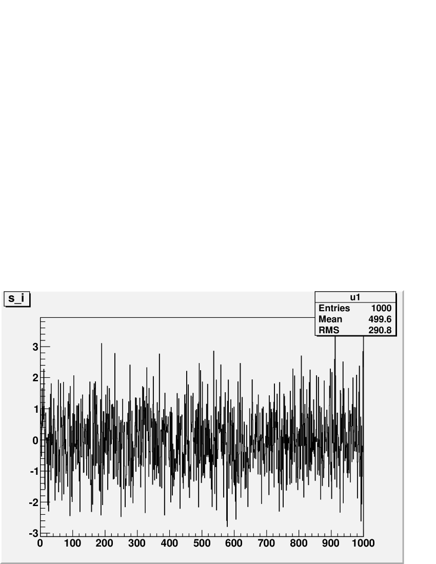
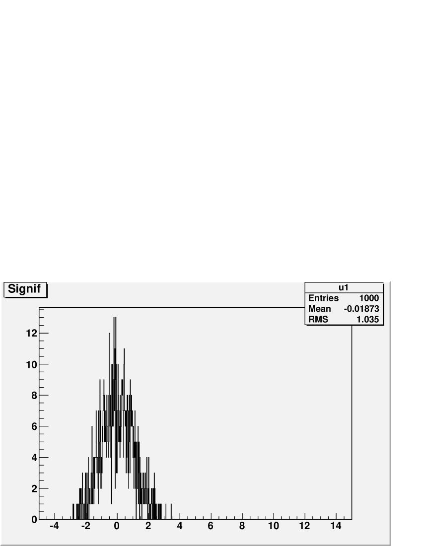
Consider the case when expected values $n_{i1}$ in the first histogram is $66$ and the expected values $n_{i2}$ in the second histogram is $45$ for each bin number $~{}i=1,2,\dots,M$. The results of the Monte Carlo experiment for this example are presented in Fig. 1.

Figure 1: Uniform distributions: the observed values $\hat{n}_{i1}$ in the first histogram (left,up), the observed values $\hat{n}_{i2}$ in the second histogram (left, down), observed significances $\hat{S}_{i}$ bin-by-bin (right, up), the distribution of observed significances (right down).

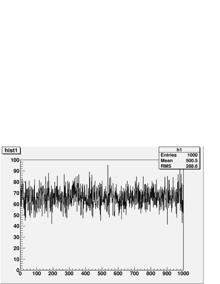
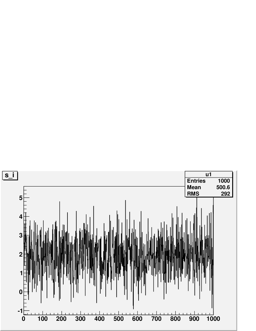
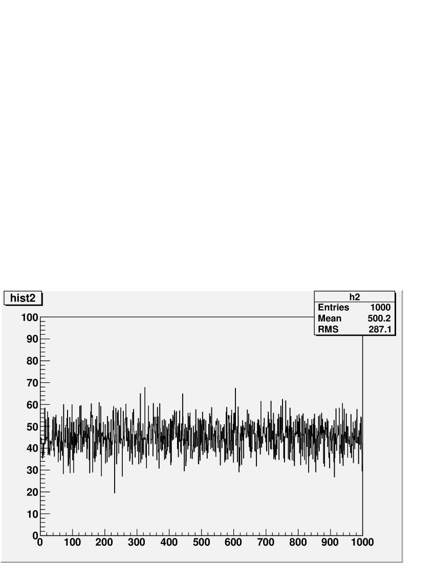
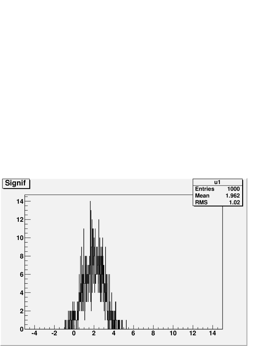
One can see that the distribution of observed significances is close to normal distribution with the $RMS~{}\sim~{}1$. The average significance is $\sim~{}1.96$, because total numbers of events in the histograms are different.

In Fig. 2 the corresponding histograms for normalized significances are shown.

Figure 2: Uniform distributions: observed normalized significances $\hat{S}_{i}$ bin-by-bin (left), the distribution of observed normalized significances (right).

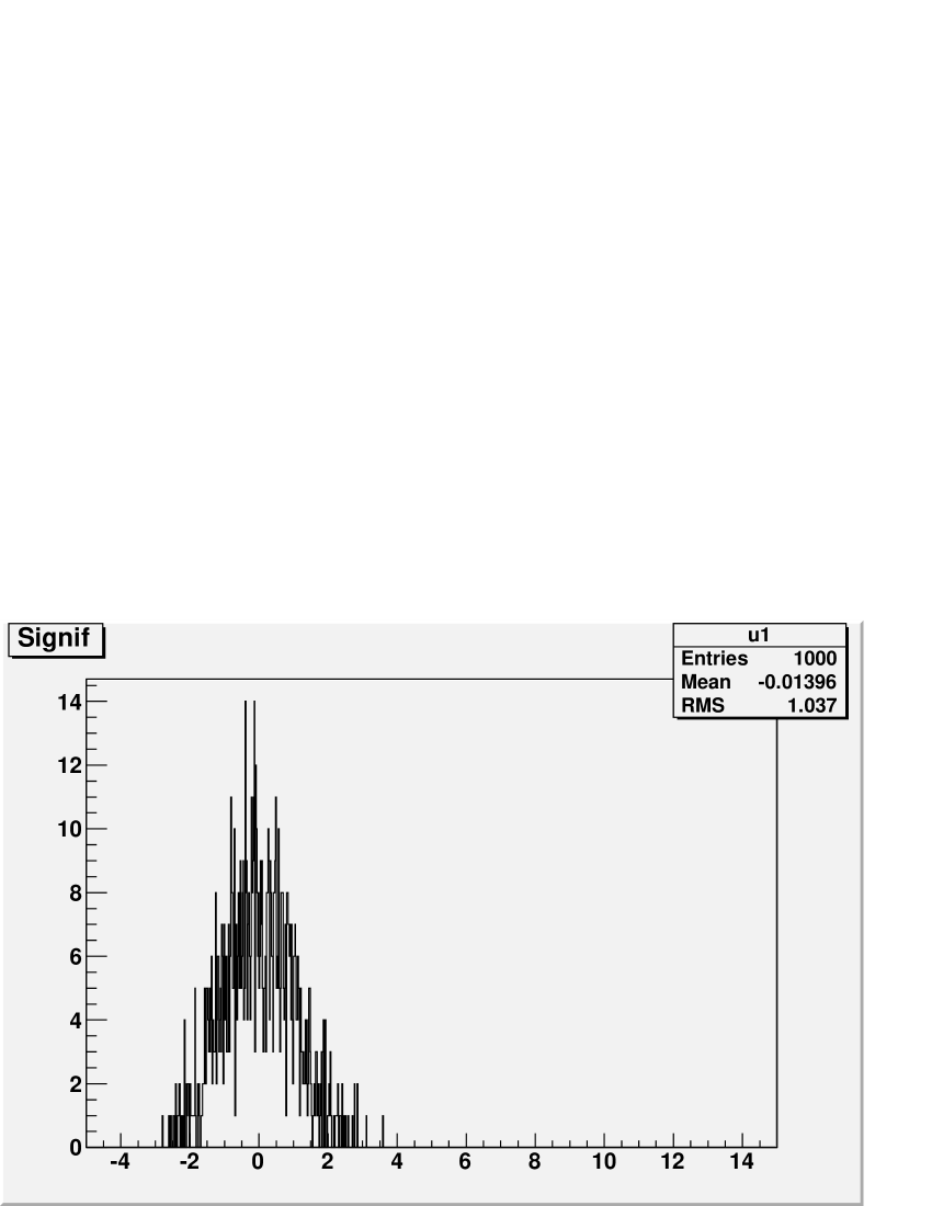
The distribution of observed normalized significance is close to standard normal distribution.

4.2 Triangle distribution

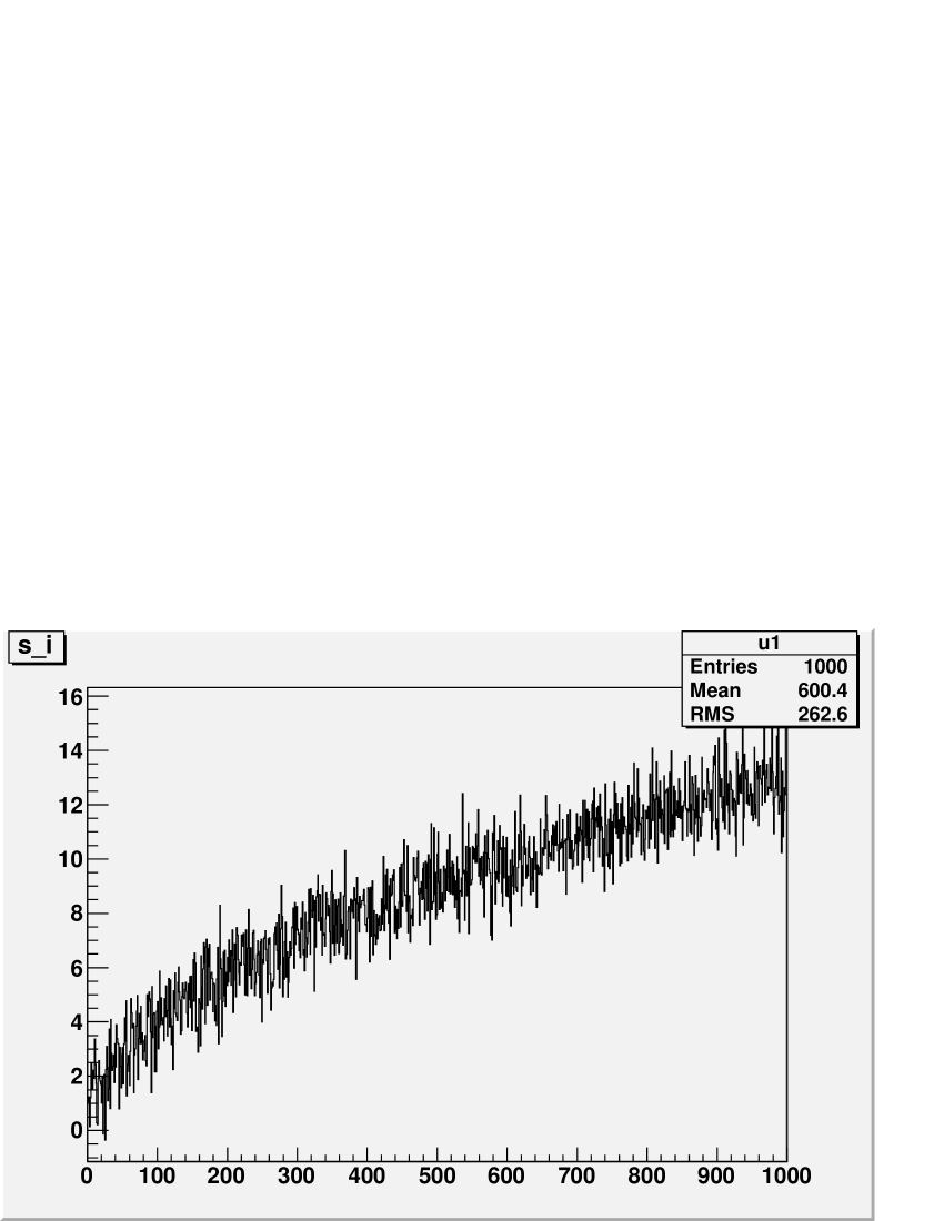
Consider the case when the expected values $n_{ik}$ in both histograms are equal to $i$, where $i$ ($i=1,2,\dots,M$) is a bin number and $k$ is a histogram number ($k=1,2$). It means that the rates of events in different bins are different. One can find that in this case the distributions of observed significances is also close to standard normal distribution, see Fig. 3. It means that the histograms which have different expected values of events in different bins give the distribution of significances close to standard normal distribution.

Figure 3: Triangle distributions: the observed values $\hat{n}_{i1}$ in the first histogram (left,up), the observed values $n_{i2}$ in the second histogram (left, down), observed significances $\hat{S}_{i}$ bin-by-bin (right, up), the distribution of observed significances (right down).

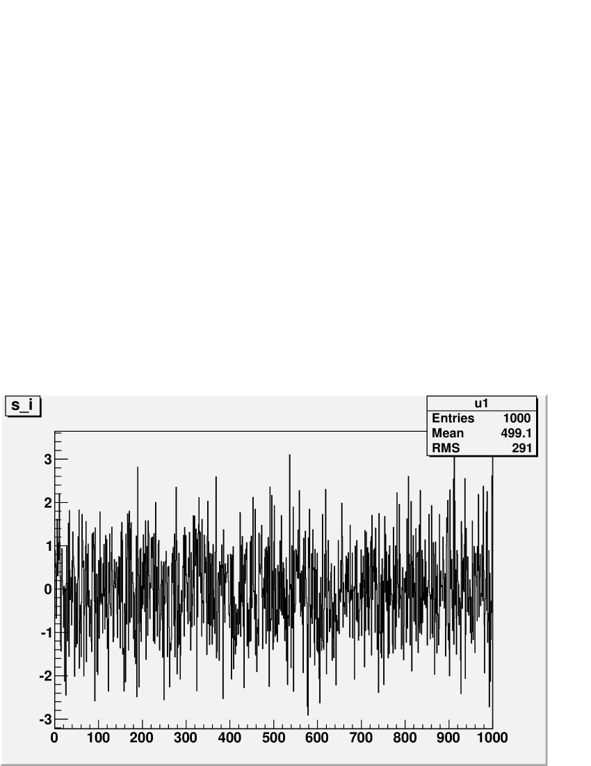
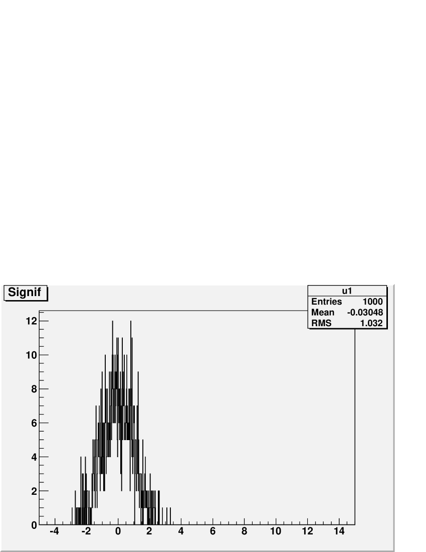
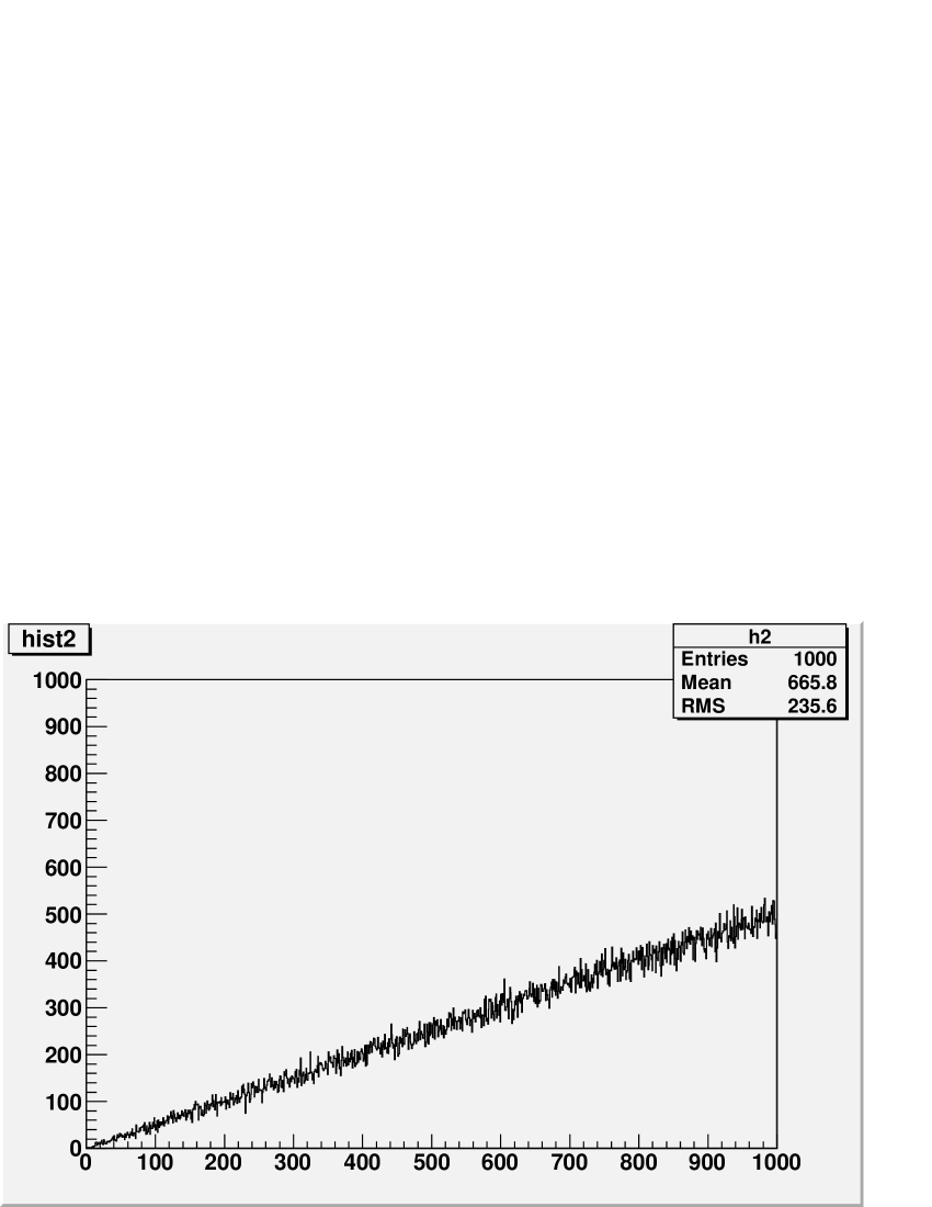
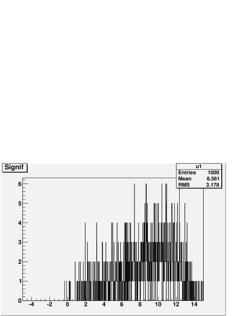
Suppose, the histograms are taken from experiments with different integrated luminosity, i.e. the total numbers of events in histograms are different. In this case the observed significances are changed from bin to bin (see, Fig. 4). Correspondingly, the distribution of significances has non-gaussian shape (in contrast with previous distributon of significances (see, Fig. 3)).

Figure 4: Triangle distributions: the observed values $\hat{n}_{i1}$ in the first histogram (left,up), the observed values $n_{i2}$ in the second histogram (left, down), observed significances $\hat{S}_{i}$ bin-by-bin (right, up), the distribution of observed significances (right down).

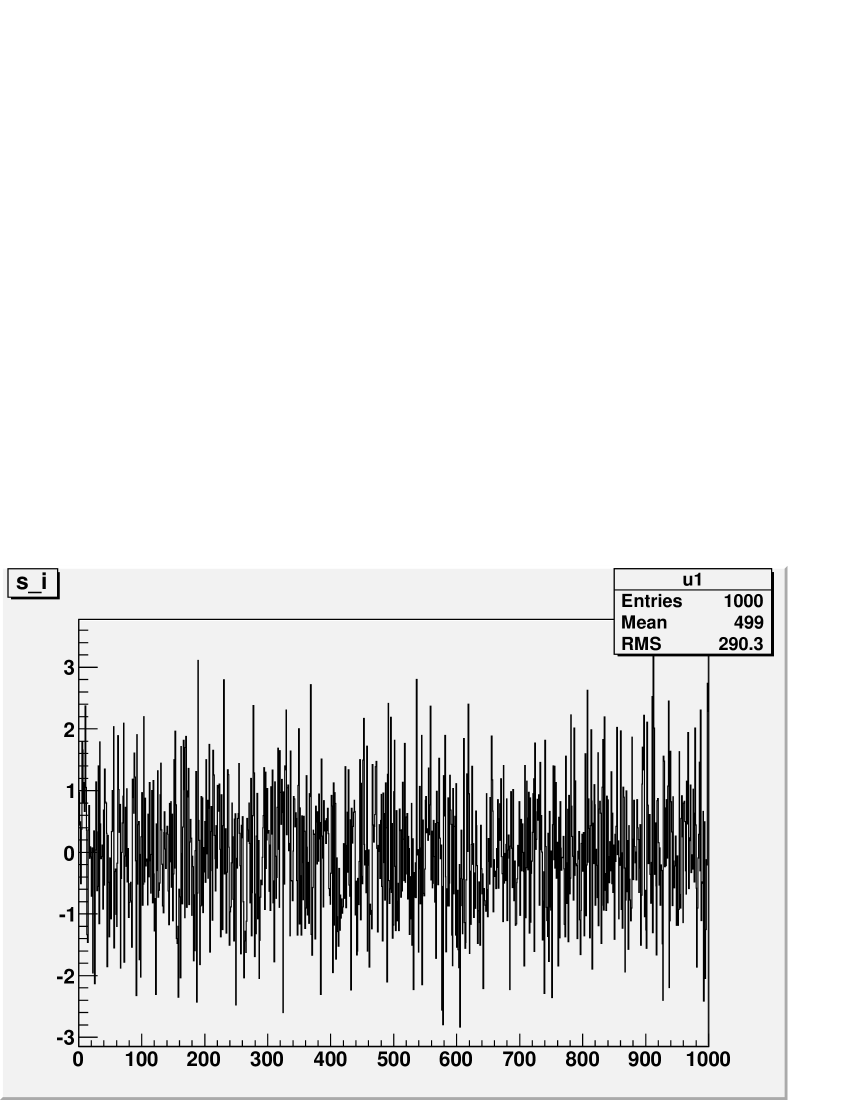
For the normalized significance (Eq. 3) we have the standard normal distribution of significances (see, Fig. 5).

Figure 5: Triangle distributions: observed normalized significances $\hat{S}_{i}$ bin-by-bin (left), the distribution of observed normalized significances (right).

So, if two histograms are obtained from the same flow of events then the distribution of the normalized significances obeys to the distribution which is close to the standard normal distribution. The $RMS$ of the distribution of significances is a measure of statistical difference between two histograms and, correspondingly, between two flows of events. This “distance measure” between two histograms has a clear interpretation:

• $RMS=0$ – histograms are identical;

• $RMS\sim 1$ – both histograms are obtained (by the using independent samples) from the same parent distribution;

• $RMS>>1$ – histograms are obtained from different parent distributions.

Note, the relation 

$$RMS^{2}=\frac{\chi^{2}}{M}-\bar{S}^{2},$$

where $\displaystyle\chi^{2}=\sum_{i=1}^{M}{\hat{S}_{i}^{2}}$, exists for the distribution of significances.

5 Resolution of the method

An accuracy (resolution) of the method depends on the number of bins $M$ in histograms, observed values in bins and, correspondingly, on the normalized coefficient $K$. The accuracy can be estimated via Monte Carlo experiments.

Two models of the statistical populations (pseudo populations) are produced. Each of models represents one of the histograms. Namely, 4999 clones for each of histograms are produced by the Monte Carlo simulation of content for each bin $i$ of histogram $k$ due to the law $N(\hat{n}_{ik},\hat{\sigma}_{ik})$. It is possible because the normal distribution is a statistically dual distribution [6]. As a result there are 5000 pairs of histograms for comparisons.

The comparison is performed for each pair of histograms (5000 comparisons). The distribution of the significances $\hat{S}_{i}$ ($\hat{S}_{i}$ is a significance of deviation for bin $i$) is obtained as a result of each comparison. After that the $RMS$, $\bar{S}$ and $\sqrt{\frac{\chi^{2}}{M}}$  are calculated.

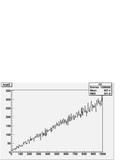
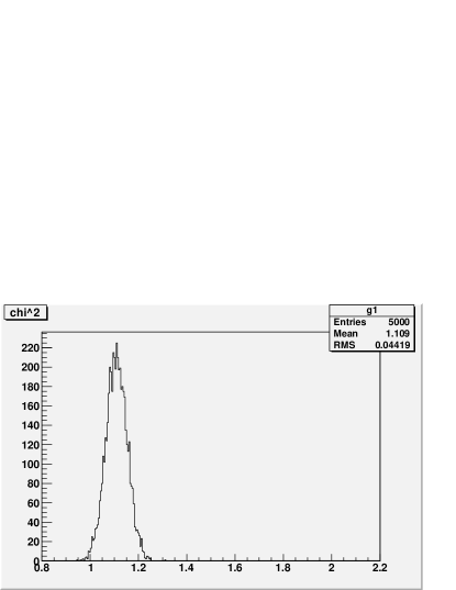
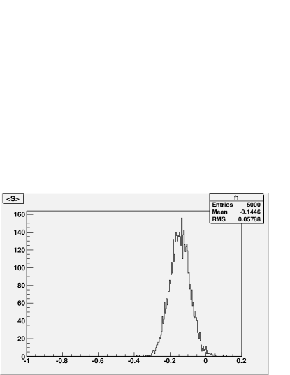
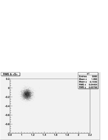
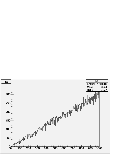
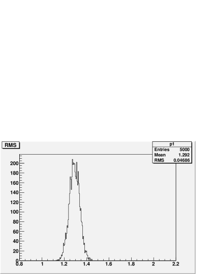
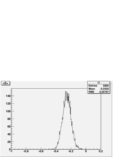
Let us consider the case (Case A) when both histograms are obtained from the same statistical population (Fig. 6). The distributions of $\sqrt{\frac{\chi^{2}}{M}}$ (Fig. 7, left), $RMS$ (Fig. 7, right), $\bar{S}$ (Fig. 8, left) and $RMS$ versus $\bar{S}$ (Fig. 8, right) are produced during 5000 comparisons of histograms.

Figure 6: Case A: input histograms – the same triangle distributions, M=300, K=1.

Figure 7: Case A: 5000 comparisons – $\sqrt{\frac{\chi^{2}}{M}}$ for each trial (left), $RMS$ for each trial (right).

Figure 8: Case A: 5000 comparisons – $\bar{S}$ for each trial (left), $RMS$ & $\bar{S}$ (right).

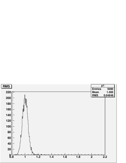
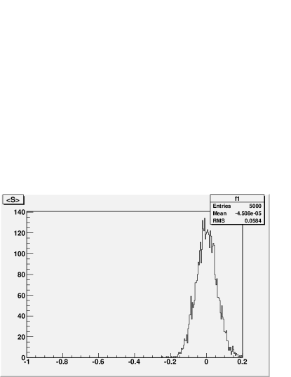
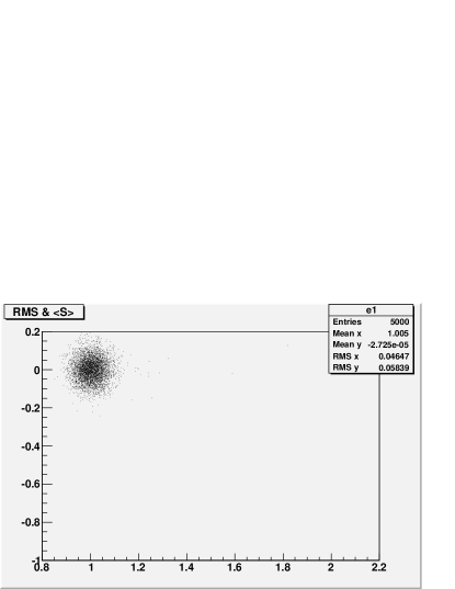
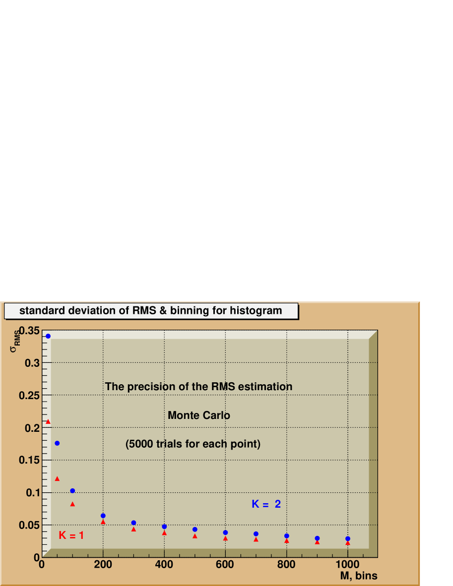
The dependencies of the resolution ($RMS$) on the number of bins $M$ and on the value of coefficient of normalization $K$ are shown in Fig. 9. Note, the resolution of $\chi^{2}$ method [1] (Fig. 7, left) practically the same as resolution of $RMS$ in this method (Fig. 7, right).

Figure 9: Triangle distributions (Sec. 4.2): the dependence of the standard deviation of RMS on number of bins $M$. This dependence is shown for two values of normalized coefficient $K$ ($K=1$ and $K=2$).

6 Distinguishability of histograms

The estimation of the distinguishability of histograms is performed with the using of hypotheses testing. “A probability of correct decision” about distinguishability of hypotheses [7] is used as measure of the potential in separation of two histograms. It is probability of the correct choice between two hypotheses “the histograms are produced by the treatment of events from the same event flow (the same statistical population)” or “the histograms are produced by the treatment of events from different event flows”. This value can characterize the distinguishability of two histograms. If $1-\kappa=1$ then the distinguishability of histograms is 100%, i.e. histograms are produced by the treatment of events from different event flows. If $1-\kappa=0$ then it is impossible to separate these histograms, i.e. histograms are produced by the treatment of events from the same event flow. The probability of correct decision $1-\kappa$ is formed by the Type I error ($\alpha$) and by the Type II error ($\beta$) in hypotheses testing. $\alpha$ (Type I error) is the probability to accept the alternative hypothesis if the main hypothesis is correct. $\beta$ (Type II error) is the probability to accept the main hypothesis if the alternative hypothesis is correct. If critical region (critical value, critical line, …) is used correctly, i.e. if $\alpha+\beta\leq 1$, then

$$1-\displaystyle\kappa=1-\frac{\alpha+\beta}{2-(\alpha+\beta)}.$$

Two additional cases are served to illustrate the estimation of distinguishability of histograms. The Case B (Fig. 10): the first histogram has a triangle distribution, the slope of the distribution in the second histogram is changed a bit with the same integral under distribution. The distributions of $\sqrt{\frac{\chi^{2}}{M}}$ (Fig. 11, left), $RMS$ (Fig. 11, right), $\bar{S}$ (Fig. 12, left) and $RMS$ versus $\bar{S}$ (Fig. 12, right) also are produced during 5000 comparisons of histograms. The Case C (Fig. 13): the first histogram has a triangle distribution, the slope of the distribution in the second histogram is changed more significantly than in the case B (integral is the same). Correspondingly, the distributions of $\sqrt{\frac{\chi^{2}}{M}}$ (Fig. 14, left), $RMS$ (Fig. 14, right), $\bar{S}$ (Fig. 15, left) and $RMS$ versus $\bar{S}$ (Fig. 15, right) are produced during 5000 comparisons of histograms.

Figure 10: Case B: input histograms – small difference between distributions, M=300, K=1.

Figure 11: Case B: 5000 comparisons – $\sqrt{\frac{\chi^{2}}{M}}$ for each trial (left), $RMS$ for each trial (right).

Figure 12: Case B: 5000 comparisons – $\bar{S}$ for each trial (left), $RMS$ & $\bar{S}$ (right).

Figure 13: Case C: input histograms – large difference between distributions, M=300, K=1.

Figure 14: Case C: 5000 comparisons – $\sqrt{\frac{\chi^{2}}{M}}$ for each trial (left), $RMS$ for each trial (right).

Figure 15: Case C: 5000 comparisons – $\bar{S}$ for each trial (left), $RMS$ & $\bar{S}$ (right).

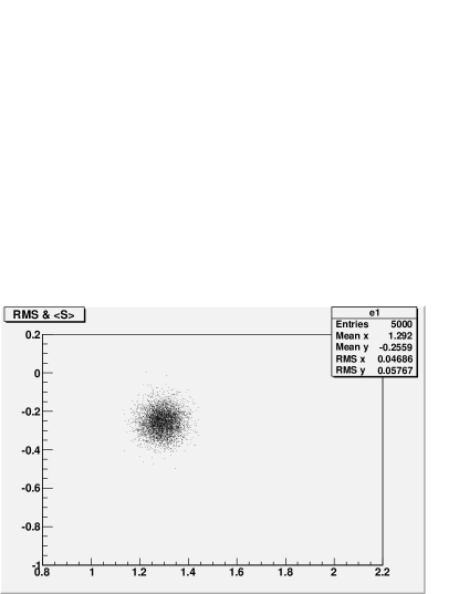
The probability of the correct decision as a measure for distinguishability of two histograms is determined by the comparison of distribution for the Case A and corresponding distribution for the Case B or Case C. The critical value is used for comparison of one-dimensional $\sqrt{\frac{\chi^{2}}{M}}$ distributions. The critical line is used for comparison of two-dimensional $RMS\&\bar{S}$ distributions. The results are presented in Tab. 1, Tab. 2, Tab. 3 and Tab. 4.

For $\chi^{2}$ method the probability of the correct decision ($1-\kappa$) about the Case realization (A or B) equals 87.26%. For another method the probability of the correct decision ($1-\kappa$) about the Case realization (A or B) equals 93.88%. One can see that the method, which uses $RMS$ and $\bar{S}$, gives better distinguishability of histograms than the $\chi^{2}$ method. Note, in this study are used only two moments of the distribution of significances (the first initial moment ($\bar{S}$) and the root from the second central moment ($RMS$)) for estimation of distinguishability of histograms.

7 Conclusions

The proposed approach allows to perform the comparison of histograms in more detail than methods which use only one test statistics. This method can be used in tasks of monitoring of the equipment during experiments. The first experience of the using the method is presented in report [8]. Note, the production of statistical (pseudo) populations, which represent the comparing histograms, allows to estimate the distinguishability of histograms in each comparison.

		In	reality
Accepted	Case A	Case B
Case A	4543	673
Case B	457	4327
$1-\kappa$	$\alpha$	$\beta$
0.8726	0.0914	0.1346

Table 1: $\sqrt{\frac{\chi^{2}}{M}}$ - 5000 decisions.

		In	reality
Accepted	Case A	Case B
Case A	4843	456
Case B	121	4544
$1-\kappa$	$\alpha$	$\beta$
0.9388	0.0242	0.0912

Table 2: $RMS\&\bar{S}$ - 5000 decisions.

		In	reality
Accepted	Case A	Case C
Case A	4982	1
Case C	18	4999
$1-\kappa$	$\alpha$	$\beta$
0.9981	0.0036	0.0002

Table 3: $\sqrt{\frac{\chi^{2}}{M}}$ - 5000 decisions.

		In	reality
Accepted	Case A	Case C
Case A	4989	0
Case C	11	5000
$1-\kappa$	$\alpha$	$\beta$
0.9989	0.0022	0.0000

Table 4: $RMS\&\bar{S}$ - 5000 decisions.