The Stagger-grid: A Grid of 3D Stellar Atmosphere Models

Abstract

Aims. We present the Stagger-grid, a comprehensive grid of time-dependent, three-dimensional (3D), hydrodynamic model atmospheres for late-type stars with realistic treatment of radiative transfer, covering a wide range in stellar parameters. This grid of 3D models is intended for various applications besides studies of stellar convection and atmospheres per se, including stellar parameter determination, stellar spectroscopy and abundance analysis, asteroseismology, calibration of stellar evolution models, interferometry, and extrasolar planet search. In this introductory paper, we describe the methods we applied for the computation of the grid and discuss the general properties of the 3D models as well as of their temporal and spatial averages (here denoted $\left\langle 3\mathrm{D}\right\rangle$ models).

Methods. All our models were generated with the Stagger-code, using realistic input physics for the equation of state (EOS) and for continuous and line opacities. Our $\sim 220$ grid models range in effective temperature, $T_{\mathrm{eff}}$, from $4000$ to $7000\,\mathrm{K}$ in steps of $500\,\mathrm{K}$, in surface gravity, $\log g$, from $1.5$ to $5.0$ in steps of 0.5 dex, and metallicity, $\left[\mathrm{Fe}/\mathrm{H}\right]$, from $-4.0$ to $+0.5$ in steps of $0.5$ and $1.0\,\mathrm{dex}$.

Results. We find a tight scaling relation between the vertical velocity and the surface entropy jump, which itself correlates with the constant entropy value of the adiabatic convection zone. The range in intensity contrast is enhanced at lower metallicity. The granule size correlates closely with the pressure scale height sampled at the depth of maximum velocity. We compare the $\left\langle 3\mathrm{D}\right\rangle$ models with currently widely applied one-dimensional (1D) atmosphere models, as well as with theoretical 1D hydrostatic models generated with the same EOS and opacity tables as the 3D models, in order to isolate the effects of using self-consistent and hydrodynamic modeling of convection, rather than the classical mixing length theory (MLT) approach. For the first time, we are able to quantify systematically over a broad range of stellar parameters the uncertainties of 1D models arising from the simplified treatment of physics, in particular convective energy transport. In agreement with previous findings, we find that the differences can be rather significant, especially for metal-poor stars.

1 Introduction

The primary source of information for stellar objects is the light they emit, which carries information about the physical conditions at its origin. However, in order to interpret the information correctly, one first needs either theoretical or semi-empirical models of the atmospheric layers at the surface of stars from where the stellar radiation escapes. Therefore, models of stellar atmospheres are essential for much of contemporary astronomy.

In the case of late-type stars, the theoretical modeling of stellar atmospheres is complicated by the presence of convective motions and turbulent flows as well as of magnetic fields in their envelopes (see review by Nordlund et al. 2009, and references therein). In particular, convection can significantly affect both the atmospheric stratification and emergent spectral energy distribution in these stars. Hence, in order to correctly represent the temperature stratifications in the outer layers of stars, from where the stellar light escapes, it is vital to accurately account for the interaction between radiative and convective energy transport at the optical surface .

The first realistic grids of line-blanketed atmosphere models for late-type stars appeared with the publication of MARCS (Gustafsson et al. 1975, 2008) and ATLAS models (Kurucz 1979; Castelli & Kurucz 2004). Subsequently, other one-dimensional (1D) atmosphere codes, e.g. PHOENIX (Hauschildt et al. 1999) and MAFAGS (Grupp 2004), were developed to model the atmospheres of stars. In general, these theoretical 1D atmosphere models assume hydrostatic equilibrium, flux constancy, and local thermodynamic equilibrium (LTE). For the modeling of convective energy transport, they commonly employ the mixing-length theory (MLT, see Böhm-Vitense 1958), which is characterized by several free parameters, the most commonly known being the mixing-length $l_{m}$, or equivalently, the parameter $\alpha_{\mathrm{MLT}}=l_{m}/H_{P}$. Alternatively, some relatives thereof are available, such as the full turbulence spectrum (FTS) theory by Canuto & Mazzitelli (1991), which itself also has a free parameter. The values of these free parameters are not known from first principles and need to be calibrated based on observations or simulations. The mixing-length theory has in total four free parameters (see Böhm-Vitense 1958; Henyey et al. 1965; Mihalas 1970). These free parameters can be calibrated based on their effect on synthetic spectra, but usually only $\alpha_{\mathrm{MLT}}$ is calibrated based on the reproduction of selected lines (Fuhrmann et al. 1993; Barklem et al. 2002; Smalley et al. 2002). Moreover, the free mixing length is calibrated in stellar evolutionary calculations by matching the observed luminosity and radius of the Sun at its current age (e.g. Magic et al. 2010). To construct simple yet realistic 1D models of convection is rather difficult, in particular convective overshooting beyond the classical Schwarzschild instability criterion is normally not considered in 1D atmospheric modeling. Attempts have been made at including its effects in 1D model atmospheres albeit with only limited success (Castelli et al. 1997).

The first numerical 1D model stellar atmosphere codes usually assumed a plane-parallel geometry for the atmospheric stratification. This was later improved upon by changing to a spherical symmetry, leading to lower temperatures in the upper layers, in particular for giant stars, due to the dilution of the radiation field with increasing radial distance, which can cover a significant fraction of the stellar radius at low $\log g$ (see Gustafsson et al. 2008). Initially line blanketing was included by means of opacity distribution functions (ODFs, Gustafsson et al. 1975) with a few hundred ODFs covering the entire spectrum, eventually replaced by opacity sampling (OS) including thousands of wavelength points (Johnson & Krupp 1976). Nowadays, thousands of ODFs or hundreds of thousands of OS wavelengths are used. Despite such high resolution in wavelength, the computational costs for 1D atmosphere models are currently quite small, at least for LTE models. Large, homogeneous grids of atmospheres with up to $\sim 10^{5}$ models exist (Gustafsson et al. 2008; Cassisi et al. 2004; Hauschildt et al. 1999), covering a wide range of stellar atmosphere parameters ($T_{\mathrm{eff}}$, $\log g$, and $\left[\mathrm{Fe}/\mathrm{H}\right]$).

Even though the 1D atmosphere models are based on numerous simplifications, they have demonstrated high predictive capabilities owing to major improvements in the atomic and molecular data (e.g. line lists by Kurucz (1993) or VALD by Piskunov et al. (1995)). Also, the continuum opacity sources and the EOS have undergone similar developments. Thanks to these, 1D atmosphere models are in many respects very successful in comparisons with observations and are widely applied in astronomy today.

Another approach, almost exclusively used for solar atmosphere modeling, is the use of semi-empirical models. In these models, the temperature stratification is inferred from observations (e.g. from lines forming at different heights or continuum center-to-limb variations). Often-used semi-empirical 1D solar atmosphere models are the Holweger & Mueller (1974), VAL3C (Vernazza et al. 1976), Maltby et al. (1986) and MISS (Allende Prieto et al. 2001) models. A similar approach can be used to integrate spatially resolved observations and thus infer the three-dimensional (3D) atmosphere structures using inversion techniques (Ruiz Cobo & del Toro Iniesta 1992; Socas-Navarro 2011). Semi-empirical modeling is rarely attempted for other stars, although exceptions exist (e.g. Allende Prieto et al. 2000).

Constructing more realistic models requires one to go beyond the 1D framework and model convection without relying on MLT. Stellar convection is an inherently 3D, time-dependent, non-local, and turbulent phenomenon. Therefore, one cannot expect 1D models to reproduce all observed properties accurately, even with access to free parameters to tweak. The next natural step is to abandon some of these crude simplifications by constructing realistic 3D atmosphere models of solar convection. Early hydrodynamic simulations (Nordlund 1982; Nordlund & Dravins 1990; Steffen et al. 1989) revealed that stellar surface convection operates in a distinctly different fashion from the MLT picture. Instead of the homogeneous convective elements, they displayed highly asymmetrical motions with slow broad steady upflows interspersed with fast narrow turbulent downdrafts, sometimes even supersonic (e.g. Stein & Nordlund 1998, hereafter SN98; Asplund et al. 2000; Nordlund et al. 2009; Carlsson et al. 2004; Ludwig et al. 1999). The advent of 3D simulations, which are constructed from first principles, has enabled astronomers to predict various observables such as solar granulation properties and spectral line profiles astonishingly well. More recent solar 3D simulations are remarkably good at reproducing the observed center-to-limb variation (e.g. Pereira et al. 2009a; Asplund et al. 2009; Ludwig 2006).

3D atmosphere models are by design free from the adjustable parameters of MLT and other parameters such as micro- and macro-turbulence that have hampered stellar spectroscopy for many decades. Instead, in 3D simulations, convection emerges naturally, by solving the time-dependent hydrodynamic equations for mass-, momentum- and energy-conservation, coupled with the 3D radiative transfer equation in order to account correctly for the interaction between the radiation field and the plasma. Also, the non-thermal macroscopic velocity fields associated with convective motions are rendered realistically, and various natural kinetic consequences such as overshooting and excitation of waves emerge from the simulations, without the need for further ad hoc modeling or additional free parameters. The inhomogeneities in the convective motions arise spontaneously and self-organize naturally to form a distinct flow pattern that exhibits the characteristic granulation at the surface. Furthermore, additional spectral observables such as limb-darkening and detailed spectral line shapes, including asymmetries and shifts, are also modeled unprecedentedly accurately with 3D models for the Sun (Nordlund et al. 2009; Pereira et al. 2009b)

For metal-poor late-type stars it has been shown (Asplund et al. 1999b; Collet et al. 2006, 2007) that the assumption of pure radiative equilibrium in the convectively stable photospheric layers of classical hydrostatic models is generally insufficient. In particular in the upper photosphere, the thermal balance is instead primarily regulated by radiative heating due to spectral line re-absorption of the continuum-radiation from below and adiabatic cooling due to the expansion of upflowing gas. In metal-poor stars, the balance between heating by radiation and cooling by mechanical expansion of the gas occurs at lower temperatures because of the weakness and scarcity of spectral lines at low metallicities. By contrast, 1D MLT models have no velocity fields outside their convection zones, and are therefore in pure radiative equilibrium. The temperature stratification there is therefore regulated solely by radiative heating and cooling, thus neglecting altogether the adiabatic cooling component. This results in an overestimation of the temperatures by up to $\sim 1\,000\,\mathrm{K}$ in 1D models at very low metallicities, which can potentially lead to severe systematic errors in abundance determinations based on 1D models (see Asplund et al. 1999b; Asplund & García Pérez 2001; Ludwig et al. 2010; Collet et al. 2009; González Hernández et al. 2010). These shortcomings of 1D models are manifested as inconsistencies in the analysis of observed spectra, such as abundance trends with excitation potential of the lines (e.g. analysis of NH lines in the very metal-poor star HE1327-2326, by Frebel et al. (2008) and discrepant abundances between atomic and molecular lines involving the same elements (e.g. Nissen et al. 2002). For further discussion, we refer to a review of possible impacts of 3D models on stellar abundance analysis by Asplund et al. (2005).

Additionally, there are discrepancies between observations and predictions from 1D models of the solar structure in the context of helioseismology, which point to mistakes in the outer layers of theoretical 1D stellar-structure models, and which are usually referred to as surface effects (Rosenthal et al. 1999). With classical 1D stellar structures, higher frequency p-modes of the Sun are systematically shifted due to discrepancies at the upper turning points of the modes, which occur in the superadiabatic peak at the top of the convection envelope. Rosenthal et al. (1999) found better agreement of stellar structures with helioseismic observations, when including the mean stratification of solar 3D models at the top, since the turbulent pressure, usually neglected in 1D models, extends the resonant cavity. Also, it was found that with 3D solar models the predicted p-mode excitation rates are much closer to helioseismic observations(Nordlund & Stein 2001; Stein & Nordlund 2001). Ludwig et al. (2009b) compared the power spectra of the photometric micro-variability induced by granulation and found good agreement between the theoretical predictions of 3D solar models and observations with SOHO.

With the aid of 3D simulations, stellar radii have been derived for a number of red giants from interferometric observations Chiavassa et al. (2010, 2012). The determined stellar radii are slightly larger than estimated with the use of 1D models, which has an impact on the zero point of the effective temperature scale derived by interferometry. Furthermore, Chiavassa et al. (2012) showed that for interferometric techniques a detailed knowledge of the granulation pattern of planet-hosting stars is crucial for the detection and characterization of exoplanets.

Several 3D magnetohydrodynamics codes with realistic treatment of radiative transfer have been developed and applied to the modeling of stellar surface convection. Here, we make use of the Stagger-code, which is developed specifically to run efficiently on the massively parallel machines available today (Nordlund & Galsgaard 1995; Kritsuk et al. 2011). The Bifrost-code is an Oslo derivative of the Stagger-code (Gudiksen et al. 2011), tailored for simulations of the solar photosphere and chromosphere, and therefore including true scattering (Hayek et al. 2010). Other widely used codes are CO⁵BOLD (Freytag et al. 2012), MURaM (Vögler et al. 2005) and ANTARES (Muthsam et al. 2010), which have been independently developed in the last decades. Beeck et al. (2012) compared solar models from three of the above 3D stellar atmosphere codes (Stagger, CO⁵BOLD and MURaM), and showed that the models are overall very similar, despite the distinct numerical approaches. Most of the available 3D stellar convection codes are now highly parallelized, which when coupled with the computational power available today makes it feasible to construct grids of 3D convection simulations within a reasonable time-scale. Grids of 2D and 3D atmosphere models already exist (Ludwig et al. 1999, 2009a; Trampedach 2007; Trampedach et al. 2013; Tanner et al. 2013). Clearly, the age of 3D atmosphere modeling has arrived, partly driven by the rising demand created by improved high-resolution spectroscopic and asteroseismic observations.

In this paper, we present a new large grid of 3D model atmospheres for late-type stars, covering an extensive range of effective temperatures, surface gravities, and metallicities. In Section 2 we describe the methods that we followed in order to compute the 3D model atmospheres, with emphasis on the convection code we used (Sect. 2.1) and on the tools we developed for scaling the grid models and post-process the results of the numerical calculations (Sect. 2.3). In Section 3, we present an overview of general properties (Sect. 3.1) of our simulations, and discuss the temporally and spatially averaged atmospheres (Sect. 3.2) from the 3D model atmospheres. We also compare our results with theoretical 1D models in Sect. 3.3 corresponding to the same stellar parameters. These have been computed with a specifically newly developed 1D code that employs exactly the same EOS and opacities as the 3D simulations. Also, we compare our 3D model atmospheres with 1D models from grids widely adopted by the astronomical community (MARCS and ATLAS). Finally, in Section 4, we summarize our findings and outline a roadmap for our future ambitions on the many possible applications of the Stagger-grid.

2 Methods

2.1 The Stagger-code

The 3D model atmospheres presented here were constructed with a custom version of the Stagger-code, a state-of-the-art, multipurpose, radiative-magnetohydrodynamics (R-MHD) code originally developed by Nordlund & Galsgaard (1995), and continuously improved over the years by its user community. In pure radiation-hydrodynamics mode, the Stagger-code solves the time-dependent hydrodynamic equations for the conservation of mass (Eq. 1), momentum (Eq. 2), and energy (Eq. 3) in a compressible flow

$$\partial_{t}\rho = -\@vec{\nabla}\cdot(\rho\@vec{v}),$$ (1)

$$\partial_{t}\rho\@vec{v} = -\@vec{\nabla}\cdot(\rho\@vec{v}\@vec{v}+\underline{\underline{\tau}})-\@vec{\nabla}p+\rho\@vec{g},$$ (2)

$$\partial_{t}e = -\@vec{\nabla}\cdot(e\@vec{v})-p\@vec{\nabla}\cdot\@vec{v}+q_{\mathrm{rad}}+q_{\mathrm{visc}},$$ (3)

coupled to the radiation field via the heating and cooling (per unit volume) term

$$q_{\mathrm{rad}} = 4\pi\rho\int_{\lambda}\kappa_{\lambda}\left(J_{\lambda}-S_{\lambda}\right)\,d\lambda,$$ (4)

which is computed from the solution of the radiative transfer equation

$$\hat{n}\cdot\@vec{\nabla}I_{\lambda} = \varrho\kappa_{\lambda}(S_{\lambda}-I_{\lambda})$$ (5)

to account properly for the energy exchange between matter and radiation (here $\rho$ denotes the density, $\@vec{v}$ the velocity field, $p$ the thermodynamic pressure, $e$ the internal energy per unit volume, $g$ the gravity, $\underline{\underline{\tau}}$ the viscous stress tensor, $q_{\mathrm{visc}}=\sum_{ij}\tau_{ij}\partial v_{i}/\partial r_{j}$ the viscous dissipation rate, $\kappa_{\lambda}$ the monochromatic opacity, $I_{\lambda}$ the monochromatic intensity, $J_{\lambda}=1/4\pi\int_{\Omega}I_{\lambda}d\Omega$ the monochromatic mean intensity averaged over the entire solid angle, and $S_{\lambda}$ the source function). We have ignored magnetic fields in the present grid of 3D convection simulations, however, we will study their effects in a future work.

2.1.1 Details on the numerics

The Stagger-code uses a sixth-order explicit finite-difference scheme for numerical derivatives and the corresponding fifth-order interpolation scheme. The solution of the hydrodynamic equations is advanced in time using an explicit third-order Runge-Kutta integration method (Williamson 1980). The code operates on a staggered, Eulerian, rectangular mesh: the thermodynamic variables, density and internal energy per volume, are cell-centered, while momentum components are defined at cell faces. Also, in the MHD mode, the components of the magnetic field $B$ (electric field $E$) are defined at the cell faces (edges). This configuration allows for a flux-conservative formulation of the magnetohydrodynamic equations, at the same time ensuring that the magnetic field remains divergence-free. The solution of the discretized equations is stabilized by hyper-viscosity which aims at minimizing the impact of numerical diffusion on the simulated flow, while providing the necessary diffusion for large-eddy simulations with finite-difference schemes (see also Nordlund & Galsgaard 1995 for further details). The values of the numerical viscosity parameters are empirically tuned for the solar surface-convection simulation: they are set large enough to stabilize the numerical solution of the hydrodynamic equations and, at the same time, kept small enough to reduce their smoothing of the flow’s structures. The same optimized values of the parameters are then applied to all other simulations in the grid.

The version of the Stagger-code we used for this work is fully MPI-parallel. The parallelization scales well with the number of cores. For this project, the simulations were typically run on $64$ cores.

2.1.2 Geometrical properties

The setup of the simulations is of the so-called box-in-a-star type: the domain of the simulations is limited to a small representative volume located around the stellar photosphere and including the top portion of the stellar convective envelope. The boundary conditions of the simulation box are periodic in the horizontal directions and open vertically. Gravity is assumed to be constant over the whole extent of the box, neglecting sphericity effects. However, since the size of the simulation domains correspond to only a fraction of the total radii of the stars ($0.4\,\%$ and $\sim 10\,\%$ of the stellar radius for the solar simulation and for a typical $\log g=1.5$ red giant simulation, respectively) such effects can be regarded as small for the purposes of the current grid of models. Also, for simplicity, the effects of stellar rotation and associated Coriolis forces are neglected in the present simulation setup, as it would add two more dimensions to the grid.

At the bottom, the inflowing material has a constant value of specific entropy per unit mass, which ultimately determines the emerging effective temperature. While the domains of our simulations cover only a small fraction of the convective zone, the box-in-a-star setup is still valid because the bulk up-flows at the bottom boundary of the simulations carry essentially the same entropy value as in deeper layers and are mostly unaffected by entrainment with cooler downflows. At the beginning of each simulation, the entropy of the inflowing gas at the bottom is adjusted in order to yield the desired $T_{\mathrm{eff}}$ and, after that, is kept unchanged during the entire run (see Sect. 2.3). Furthermore, pressure is assumed to be constant over the whole bottom layer.

The physical dimensions in the horizontal directions are chosen to be large enough to cover an area corresponding to about ten granular cells. The vertical dimensions are extended enough for the simulations to cover at least the range of $-5.0<\log\tau_{\mathrm{Ross}}<+6.0$ in terms of Rosseland optical depth (in fact they range on average from $-7.3<\log\tau_{\mathrm{Ross}}<+7.5$), which typically corresponds to approximately six orders of magnitude in pressure (about 14 pressure scale heights). All of the simulations have a mesh resolution of $240^{3}$, since a resolution of about $200^{3}-250^{3}$ was found to be adequate (see Asplund et al. 2000). Five layers at the bottom and the top are reserved for the so-called ghost-zones: these extra layers serve to enforce boundary conditions for the high-order derivatives in the vertical direction. The spacing between cells in the horizontal direction ($\Delta x,\Delta y$) is constant, ranging from about 6 km in dwarfs to about 25 Mm in giants, while it varies smoothly with depth in the vertical direction, in order to resolve the steep temperature gradients near the optical surface. These are the layers from where the continuum radiation escapes; they are characterized by a sharp transition between stellar interior and outer layers in terms of thermodynamic quantities such as temperature, internal energy, and entropy that marks the beginning of the photosphere. Also, the steepest temperature gradients are found in the superadiabatic region just below the optical surface ($0.0<\log\tau_{\mathrm{Ross}}<2.0$). Therefore, it is very important that the thin transition layer around the optical surface is well-resolved in order to ensure an accurate modeling of the radiative transfer and to avoid spurious numerical artifacts from insufficient spatial resolution.

2.1.3 Equation of state

We use the realistic equation of state (EOS) by Mihalas et al. (1988), which explicitly treats excitation to all bound states of all ionization stages, of all included elements. We have custom computed tables for a mix of the 17 most abundant elements ($\mathrm{H},\mathrm{He},\mathrm{C},\mathrm{N},\mathrm{O},\mathrm{Ne},\mathrm{Na},\mathrm{Mg},\mathrm{Al},\mathrm{Si},\mathrm{S},\mathrm{Ar},\mathrm{K},\mathrm{Ca},\mathrm{Cr},\mathrm{Fe}$ and $\mathrm{Ni}$). The only molecules that are included in the EOS are $\mathrm{H}_{2}$ and $\mathrm{H}_{2}^{+}$, and they are treated on equal footing with the atoms and ions. For the solar abundances we employed the latest chemical composition by Asplund et al. (2009), which is based on a solar simulation performed with the same code and atomic physics as presented here. Our choice for the EOS, is supported by Di Mauro et al. (2002) who showed that solar models based on the EOS by Mihalas et al. (1988) show better agreement with helioseismology in the outer $20\,\mathrm{Mm}$ ($\geq 0.97\,R_{\odot}$), compared to models based on the OPAL-EOS. We inverted the Mihalas et al. (1988) EOS tables, hence the temperatures and the thermodynamic pressures are tabulated as a function of density and internal energy. This inversion exploits the analytical derivatives provided in the EOS tables to minimize losses in accuracy. These analytical derivatives are also used in the bi-cubic spline interpolation in the inverted tables.

2.1.4 Opacity

We use the continuum absorption and scattering coefficients listed in detail and with references by Hayek et al. (2010). These include the sophisticated calculations by Nahar (2004) for the first three ions of all metals we include, except for $\mathrm{K}$ and $\mathrm{Cr}$. These calculations are improvements over those forming the basis for the OP opacities (Badnell et al. 2005). The line opacity is supplied by the opacity sampling (OS) data that was also used for the newest MARCS grid of stellar atmospheres Gustafsson et al. (2008), which are in turn based on the VALD-2 database (Stempels et al. 2001) of atomic and molecular lines.

2.1.5 Radiative transfer

The radiative heating and cooling rate (Eq. 4) is evaluated by solving the radiative transfer equation

$$\frac{dI_{\lambda}}{d\tau_{\lambda}}=I_{\lambda}-S_{\lambda},$$ (6)

where $\tau_{\lambda}=\int\rho\kappa_{\lambda}ds$ denotes the monochromatic optical depth along a given direction $s$, with a method similar to that by Feautrier (1964). The equation is solved at each time step and grid point on long characteristics, along the vertical direction and along eight additional inclined angles (two $\mu=\cos\theta$ and four $\varphi$-angles) by tilting the (domain-decomposed) 3D cube. Given the opacity $\kappa_{\lambda}$ and the source function $S_{\lambda}$, the monochromatic intensity $I_{\lambda}$ can be obtained by solving Eq. (6) and the radiative heating and cooling rate computed by integrating $\rho\kappa_{\lambda}(I_{\lambda}-S_{\lambda})$ over solid angle and wavelength. We use the Radau quadrature to determine the optimal ray directions to approximate the angular integral in the calculation of the radiative heating and cooling rate as a weighted sum. For the radiative transfer calculations, we employ opacities as described above (Sect. 2.1.4).

Computing the full monochromatic solution to the radiative transfer equation in 3D at each time step is extremely expensive. The cost of the radiative transfer calculations however can be reduced enormously by opting instead for an approximated solution based on the opacity binning or multi-group method (Nordlund 1982; Skartlien 2000). Following this method, we sort all sampled wavelength points into different bins based on the spectral range they belong to and on their associated opacity strength or, better, their formation depth, i.e. the Rosseland optical depth $\tau_{\mathrm{Ross}}\left(\tau_{\lambda}=1\right)$, where the monochromatic optical depth equals unity. In this way, wavelength points characterized by similar formation heights and belonging to the same spectral interval are grouped together (see Fig. 3). For each simulation, we use the 1D temporal and spatial mean stratification to estimate the formation heights of the various wavelengths and sort the wavelengths into the different opacity bins. The bin selection and wavelength sorting process is performed twice during the simulation’s relaxation phase after updating the individual mean stratifications, but is kept unchanged during the production runs that make up the time-series presented in this work.

To each bin, we assign a mean opacity $\kappa_{i}$ which accounts for the contribution from both continuum and line opacities. To compute the mean opacities, we differentiate between diffusion and free-streaming limits, i.e. between the optical thick and optical thin regimes, below and above the photospheric transition zone, respectively. The mean bin-opacity $\kappa_{i}$ is calculated as a Rosseland-like average

$$\kappa_{\mathrm{Ross},i}=\left.\int_{\lambda\left(i\right)}\frac{dB_{\lambda}}{dT}d\lambda\middle/\int_{\lambda\left(i\right)}\frac{1}{\kappa_{\lambda}}\frac{dB_{\lambda}}{dT}d\lambda\right.$$ (7)

in the optical thick regime, and as a mean-intensity-weighted mean opacity

$$\kappa_{J,i}=\left.\int_{\lambda\left(i\right)}\kappa_{\lambda}J_{\lambda}d\lambda\middle/\int_{\lambda\left(i\right)}J_{\lambda}d\lambda\right.$$ (8)

in the optical thin regime, where $\lambda\left(i\right)$ is the set of wavelength points assigned to bin $i$. For bin $i$, the transition from one regime to the other around that bins optical surface is achieved by means of an exponential bridging of the two averages:

$$\kappa_{i}=e^{-2\tau_{\mathrm{Ross},i}}\kappa_{J,i}+\left(1-e^{-2\tau_{\mathrm{Ross},i}}\right)\kappa_{\mathrm{Ross},i}.$$ (9)

All simulations presented here have been run with the radiative transfer in the strict LTE approximation, i.e. under the assumption that he monochromatic source function $S_{\lambda}$ (in Eq. 4) is the Planck function at the local gas temperature, i.e. $S_{\lambda}\left(T\right)=B_{\lambda}\left(T\right)$. For each bin $i$, we compute an integrated source function by summing up the contributions from all wavelength points in the bin;

$$S_{i}=B_{i}=\int_{\lambda(i)}B_{\lambda}d\lambda$$ (10)

Collet et al. (2011) showed that, with this opacity binning implementation, the approximation of strict LTE results in a temperature stratification very similar to the case, where scattering is properly treated, as long as the contribution of scattering to the extinction is excluded when averaging the mean opacities $\kappa_{J,i}$ (Eq. 8) in the optically thin layers ("streaming-regime"), but include it as true absorption when averaging the mean opacities $\kappa_{\mathrm{Ross},i}$ (Eq. 7) in the optically thick layers ("diffusion approximation regime."). They also showed that including scattering as true absorption leads to erroneous atmosphere structures due to overestimated radiative heating in the optically thin layers. However, these findings have so far being verified only a small sample of stellar parameters, therefore we cannot rule out that scattering needs to be accounted for properly in certain cases. Nonetheless, evaluating the radiative transfer in strict LTE greatly eases the computational burden compared to the case, where the contribution of scattering is included to the total extinction (Hayek et al. 2010).

The radiative transfer equation is solved for the individual opacity bins (Eq. 5) for all layers that have $\max\left(\tau_{\mathrm{Ross}}\right)<300$, while in the deeper layers, we use instead the diffusion approximation, which is fulfilled to a high degree at such depths. With the opacity binning approximation, the radiative heating rate term (Eq. 4) takes then the form

$$q_{\mathrm{rad}} = 4\pi\rho\sum_{i}\kappa_{i}\left(J_{i}-B_{i}\right)$$ (11)

where $J_{i}$ is the mean intensity computed from the solution of the radiative transfer equation for bin $i$.

For the relaxation phase of the simulation runs we considered six bins, while for the final models we used twelve opacity bins. We have developed an algorithm for the bin selection, which will be explained further below (see Sect. 2.3.2). Towards lower surface gravities ($\log g\lesssim 2.0$) and higher effective temperatures, numerical artifacts in the radiative transfer can occasionally develop and manifest as a Moiré pattern in the integrated outgoing intensities due to very steep temperature gradients in the photosphere. For those situations, we solve the radiative transfer equation on an adaptive mesh with finer vertical resolution, which is dynamically optimized to resolve regions where temperature gradients are steeper. The radiative heating and cooling rates computed on the adaptive mesh are then interpolated back to the coarser hydrodynamic depth scale under the consideration of energy conservation.

2.2 The Stagger-grid models

Figure 1: Kiel diagram ($T_{\mathrm{eff}}-\log g$ diagram) showing the targeted Stagger-grid parameters for the 217 models, comprising seven different metallicities (colored circles). Four additional standard stars (see text) are also indicated (squares). In the background, the evolutionary tracks for stellar masses from $0.7$ to $1.5\,M_{\odot}$ and for solar metallicity are shown (thin grey lines).

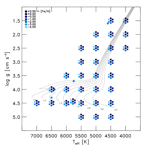
The Stagger-grid covers a broad range in stellar parameters with 217 models in total. The range in effective temperature is from $T_{\mathrm{eff}}=4000\,\mathrm{K}$ to $7000\,\mathrm{K}$ in steps of $500\,\mathrm{K}$, while the gravity ranges from $\log g=1.5$ to $5.0$ in steps of $0.5$. The grid also covers a broad range in metallicity starting from $\left[\mathrm{Fe}/\mathrm{H}\right]=-4.0$ to $+0.5$ in steps of $1.0$ below $-1.0$, and steps of $0.5$ above that. We decided to apply the same parameters $T_{\mathrm{eff}}$ and $\log g$ for all metallicities, in order to facilitate the interpolation of (averaged) models within a regular grid in stellar parameters. In addition, the grid also includes the Sun with its non-solar metallicity analogs, and four additional standard stars, namely HD 84937, HD 140283, HD 122563 and G 64-12 that are presented in Bergemann et al. (2012). For metal-poor chemical compositions with $\left[\mathrm{Fe}/\mathrm{H}\right]\leq-1.0$ we applied an $\alpha$-enhancement of $\left[\alpha/\mathrm{Fe}\right]=+0.4\,\mathrm{dex}$, in order to account for the enrichment by core-collapse supernovae (Ruchti et al. 2010).

In Figure 1, we present an overview of our simulations in stellar parameter space. Therein, we also show evolutionary tracks (Weiss & Schlattl 2008) for stars with masses from $0.7$ to $1.5\,M_{\odot}$ and solar metallicity, in order to justify our choice of targeted stellar parameters. Hence, the grid covers the evolutionary phases from the main-sequence (MS) over the turnoff (TO) up to the red-giant branch (RGB) for low-mass stars. In addition, the RGB part of the diagram in practice also covers stars with higher masses, since these are characterized by similar stellar atmospheric parameters.

2.3 Scaling and relaxing 3D models

Generating large numbers of 1D atmosphere models is relatively cheap in terms of computational costs, but the same is not true for 3D models. Based on our experiences from previous simulations of individual stars, we designed a standard work-flow of procedures for generating our grid. More specifically, we developed a large set of IDL-tools incorporating the various necessary steps for generating new 3D models, which we then applied equally to all simulations. The steps are:

• Scale the starting model from an existing, relaxed 3D simulation, and perform an initial run with six opacity bins, so that the model can adjust to the new stellar parameters.

• Check the temporal variation of $T_{\mathrm{eff}}$ and estimate the number of convective cells. If necessary, adjust the horizontal sizes, in order to ensure that the simulation box is large enough to enclose at least ten granules.

• If the optical surface has shifted upwards during the relaxation, add new layers at the top of it to ensure that $\left\langle\log\tau_{\mathrm{Ross}}\right\rangle_{\mathrm{top}}<-6.0$.

• Determine the period $\pi_{0}$ of the radial p-mode with the largest amplitude, then damp these modes with an artificial exponential-friction term with period $\pi_{0}$ in the momentum equation (Eq. 2).

• Let the natural oscillation mode of the simulation emerge again by decreasing the damping stepwise before switching it off completely.

• Re-compute the opacity tables with 12 bins for the relaxed simulation.

• Evolve the simulations for at least $\sim 7$ periods of the fundamental p-mode, roughly corresponding to $\sim 2$ convective turnover times, typically, a few thousand time-steps, of which 100 – 150 snapshots equally spaced were stored and used for analysis.

During these steps the main quantities of interest are the time evolution of effective temperature, p-mode oscillations, and drifts in the values of the mean energy per unit mass and of the mean density at the bottom boundary, which indicate the level of relaxation. When the drifts in these above properties stop, we regard the simulation as relaxed. If these conditions were not fulfilled, we continued running the model, to give the simulation more time to properly adjust towards its new quasi-stationary equilibrium state. Also, when the resulting effective temperature of an otherwise relaxed simulation deviated more than 100 K from the targeted $T_{\mathrm{eff}}$, we re-scaled the simulation to the targeted value of $T_{\mathrm{eff}}$ and started over from the top of our list of relaxation steps.

The interplay between EOS, opacities, radiative transfer and convection can shift the new location of the photosphere, when the initial guess made by our scaling procedure slightly misses it. This is the case for a few red giant models leading to upwards-shifts of the optical surface and of the entire upper atmosphere during the adjustment phase after the scaling, with the average Rosseland optical depth ending up to be larger than required, i.e. $\left\langle\log\tau_{\mathrm{Ross}}\right\rangle_{\mathrm{top}}\geq-6.0$. In order to rectify this, we extended those simulations at the top by adding extra layers on the top, until the top layers fulfilled our requirements of $\left\langle\log\tau_{\mathrm{Ross}}\right\rangle_{\mathrm{top}}<-6.0$.

2.3.1 Scaling the initial models

To start a new simulation, we scale an existing one with parameters close to the targeted ones, preferably proceeding along lines of constant entropy of the inflowing gas at the bottom in stellar parameter space (see Fig. 6). In this way, we find that the relaxation process is much faster. In order to generate an initial model for a set of targeted parameters, we scale temperature, density, and pressure with depth-dependent scaling ratios derived from two 1D models, with parameters corresponding to the current and intended 3D model (Ludwig et al. 2009a). For this, we used specifically computed 1D envelope models (MARCS or our own 1D models, see Sect. 3.3.1), which extend to $\log\tau_{\mathrm{Ross}}>4.0$. The reference depth-scale for all models in the scaling process is the Rosseland optical depth above the photosphere and gas pressure normalized to the gas pressure at the optical surface below it ($\log\tau_{\mathrm{Ross}}>0.0$).

Figure 2: In the top panel, we display the non-equidistant vertical spacing $\Delta z$ of the depth scale as a function of geometrical depth in our solar model (solid line). The $z$-scale is optimized to resolve the flows and thermal structure, which naturally results in the highest spatial resolution around the photosphere. Furthermore, we also show the maximum of the vertical gradient of the absorption coefficient $\max\left\langle d\ln\alpha_{\mathrm{Ross}}/dz\right\rangle$ as a function of depth (dotted line). In the bottom panel, we show the aspect ratio $\Delta z/\Delta x$ (solid line) and we also indicated its lower allowed limit with $1:4$ (dashed line). The actual vertical-to-horizontal aspect ratio ranges from $0.26$ at the photosphere to $1.18$ at the bottom of the simulation domain.

After the initial scaling, we construct the geometrical depth scale $z$ for the new simulation by enforcing the same (quasi-)hydrostatic-equilibrium condition as in the starting simulation, but with the newly scaled pressure and density. The resulting new $z$-scale is usually not smooth, therefore we generate a new $z$-scale, which is optimized to resolve the region with the steepest (temperature) gradients, as shown in Fig. 2. The density-, energy-, and velocity cubes are then interpolated to this new geometrical depth scale. The new $z$-scale is constructed using the variation with depth of the (smoothed) maximum of the derivative of the Rosseland absorption coefficient, $\max\left\langle d\ln\alpha_{\mathrm{Ross}}/dz\right\rangle$, as a guide. The basic idea behind this approach is to vertically distribute the mesh points as evenly as possible on the optical-depth scale. With such an optimized $z$-scale we can efficiently resolve the same features with fewer grid-points, compared to an equidistant vertical mesh. Furthermore, a limiting vertical-to-horizontal aspect ratio ($\Delta z/\Delta x$ and $\Delta z/\Delta y$) of $1:4$ over the whole vertical extent is enforced. We find that this value represents in practice an optimal lower limit to the aspect ratio, with respect to numerical stability and accuracy of the solution of the radiative transfer equation along inclined rays. Finally, the position of the zero-point in the depth scale is adjusted to coincide with the position of the mean optical surface, i.e. $\left\langle\tau_{\mathrm{Ross}}\right\rangle_{\left(z=0\right)}=1$.

At fixed surface gravity and metallicity, the mean diameter of the granules, which is used for determining the horizontal extent of the simulation, increases with higher effective temperature (see Figs. 11 and Sect. 3.1.5). The number of granules present in the simulation box is retrieved with the aid of the contour routine in IDL. Based on the map of the temperature below the surface (the vertical velocity would serve equally well), a contour chart of the significantly hotter granules is extracted, from which the number of granules is counted. Concerning the temporal resolution of the simulation sequences of the final production runs, the frequency, at which snapshots are stored, is based on the sound-crossing time of one pressure scale height, $H_{P}$, in the photosphere, i.e.

$$\Delta t_{\mathrm{snap}} = \left\langle H_{P}/c_{s}\right\rangle_{\left(\tau=2/3\right)}$$ (12)

(see Cols. 14 and 15 in Table 4). With the help of functional fits of the dependence of granule sizes and sound-crossing time scales on stellar parameters, the horizontal sizes of the simulation boxes and the snapshot sampling times can be estimated rather accurately in advance (see App. B).

2.3.2 Selection of the opacity bins

Figure 3: We show the twelve opacity bins selected for the solar simulation by plotting the opacity strength (or, more precisely, the formation height) against wavelength for all sampled wavelength points. The individual bin elements are indicated by colored symbols. For clarity, we plotted only a subset of the wavelength points considered for the opacity binning procedure. In the background, we included the smoothed histogram of the opacity strength distribution (blue contour). This shows how the majority of $\lambda$-points are mostly concentrated close to the continuum-forming layers and only a smaller fraction contributes to lines.

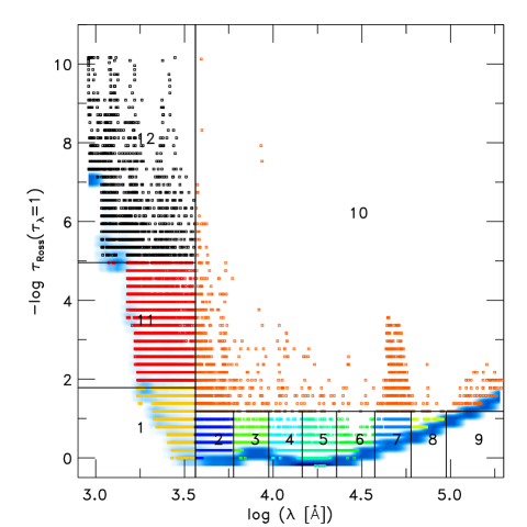
As we mentioned earlier, in Sect. 2.1.5, the purpose of the opacity-binning approximation is to reproduce the radiative heating and cooling rates as accurately as possible with a small number of opacity-bins, in order to reduce the computational burden. For the assignment of wavelength points to bins, we first compute the opacity strengths for all of the $\gtrsim 10^{5}$ wavelength points in the opacity-sampling (OS) data from the MARCS package (Gustafsson et al. 2008). The histogram of their distribution as a function of wavelength (see Fig. 3) exhibits a characteristic "L"-shape. Shorter wavelengths (UV) require more bins to resolve the wide range in opacity strength, while the lower part of the L-shaped distribution at longer wavelengths (optical and IR) calls for a better resolution in terms of wavelength. Therefore, we initially make a division in wavelength at $\lambda_{X}$, between the UV and the optical/IR (see boundaries of bin 1, 11 and 12 in Fig. 3) and comprising approximately an equal number of wavelength points. These two regions are then in turn subdivided evenly into opacity bins according to the number of $\lambda$-points. By trial and error, we found that a binning scheme with three bins in the $\lambda<\lambda_{X}$ region and eight bins for $\lambda>\lambda_{X}$, one of which being a large one and comprising the stronger lines in the optical and IR (bin number 10 in Fig. 3) gives a good representation of the monochromatic radiative heating and cooling. We iterate the bin selection with slight differences (e.g., one additional division in opacity strength for the 8 bins in the lower part of the optical and IR) and by small adjustments, and choose the bin selection with the smallest relative difference between the total heating rates computed with opacity binning $q_{\mathrm{bin}}$ and the full monochromatic solution $q_{\lambda}$ for the average stratification of the 3D simulation, i.e.

$$\max\left[\delta q_{\mathrm{bin}}\right]=\frac{\max\left|q_{\mathrm{bin}}-q_{\lambda}\right|}{\max\left|q_{\lambda}\right|}.$$ (13)

We found that the individual selection of some of the bins displays a highly non-linear response to small changes. In most cases an even distribution was favored by the minimization. Naturally, our method will typically find only a local minimum due to the small sample of iterations instead of a true global minimum. However, our method is a fast, repeatable, and automatic selection of the opacity bins, which minimizes the human effort significantly, while at the same time yielding very satisfactory results. Moreover, the possible deviation from the global minimum due to our automated bin selection and its resulting uncertainties are anyways smaller than the overall uncertainties associated with the opacity binning method.

Figure 4: Comparison of the radiative heating and cooling resulting from monochromatic computations $q_{\lambda}$ (filled dots) and the opacity binning method $q_{\mathrm{bin}}$ (solid line) for the solar model mean stratification. In the top panel we show both $q_{\mathrm{rad}}$ vs. optical depth, while in the bottom panel, we compare the two against each other.

In Fig. 4, we compare the resulting radiative heating and cooling rates from the monochromatic calculation against those from the opacity binning solution for the mean stratification of our solar model. The radiative heating and cooling rates from the simplified opacity binning appear rather similar to those from the monochromatic solution, thereby supporting our approach. For the solar model, our algorithm finds a bin selection that is just slightly less accurate ($\max\left[\delta q_{\mathrm{bin}}\right]=2.78\,\%$) than an optimized manual bin selection ($1.86\,\%$). Incidentally, with six bins, we get $\max\left[\delta q_{\mathrm{bin}}\right]=3.54\,\%$. We obtain an average $\max\left[\delta q_{\mathrm{bin}}\right]$ for all the grid models of $\overline{\max\left[\delta q_{\mathrm{bin}}\right]}=2.38\,\%$, while with six bins we get $\overline{\max\delta q_{\mathrm{bin}}}=3.0\,\%$. We find that $\max\left[\delta q_{\mathrm{bin}}\right]$ increases slightly with $T_{\mathrm{eff}}$ and $\left[\mathrm{Fe}/\mathrm{H}\right]$. We note that the opacity binning method with its small number of bins states an approximation for the radiative transfer, therefore, despite the small values for $\max\left[\delta q_{\mathrm{bin}}\right]$ further improvement is necessary.

3 Results

The spatially and temporally averaged mean 3D stratifications (hereafter $\left\langle 3\mathrm{D}\right\rangle$) from all of our 3D models will be available online. The methods we applied to average our models are explicitly described in a separate paper. We provide the models in our own format, but also in various commonly used formats suited for standard 1D spectrum synthesis codes such as MOOG (Sneden 1973), SYNTHE (Kurucz 1993) and Turbospectrum (Plez 2008; de Laverny et al. 2012), together with routines to interpolate the $\left\langle 3\mathrm{D}\right\rangle$ models to arbitrary stellar parameters. In this paper the discussion will be confined to global properties and mean stratifications only. More extensive discussions and presentations of the wealth of details present in the data of our 3D RHD models will be performed systematically in subsequent papers.

3.1 Global properties

In Table 4, we have listed the stellar parameters together with the thermodynamic values fixed for the inflows at the bottom, i.e. the internal energy $\varepsilon_{\mathrm{bot}}$, density $\rho_{\mathrm{bot}}$ and entropy $s_{\mathrm{bot}}$, as well as important global properties for our 3D simulations. Before we consider the $\left\langle 3\mathrm{D}\right\rangle$ stratifications in Sect. 3.2, we briefly discuss some (temporally averaged) global properties.

3.1.1 Stellar parameters

Surface gravity and metallicity are input parameters for a simulation, while the effective temperature is a property ensuing from the fixed entropy of the inflowing material at the bottom $s_{\mathrm{bot}}$. We calculate the effective temperature from the spatially averaged emergent radiative energy flux $F_{\mathrm{rad}}$ and the Stefan-Boltzmann law $T_{\mathrm{eff}}=\left[F_{\mathrm{rad}}/\sigma\right]^{1/4}$, with $\sigma$ being the Stefan-Boltzmann constant. In Column 1 of Table 4 we have listed the resulting temporally averaged $T_{\mathrm{eff}}$ of our final, relaxed simulations. These differ somewhat from the targeted $T_{\mathrm{eff}}$s, since we do not know a priori, the relation between $s_{\mathrm{bot}}$ and $T_{\mathrm{eff}}$. However, the majority of our models ($72\%$) deviate less than 50K, and the mean deviation for the whole grid is $\overline{\Delta T_{\mathrm{eff}}}\sim 32\,\mathrm{K}$.

3.1.2 Constant entropy of the adiabatic convection zone

Figure 5: Overview of the constant entropy value of the adiabatic convection zone, which is given by the fixed entropy of the inflowing plasma at the bottom, $s_{\mathrm{bot}}$, (circles) as well as the atmospheric entropy minimum, $s_{\mathrm{min}}$, (squares) for two metallicities ($\left[\mathrm{Fe}/\mathrm{H}\right]=-0.5$ and $0.0$, blue and black respectively) against $T_{\mathrm{eff}}$. The jump in entropy, $\Delta s$, is indicated with vertical dotted lines. Simulations with the same gravity are connected with functional fits for $s_{\mathrm{bot}}$ and $s_{\mathrm{min}}$ (solid and dashed lines respectively; see App. B), while similar simulations with different $\left[\mathrm{Fe}/\mathrm{H}\right]$ are connected with short solid black lines.

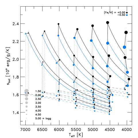
The main input parameter that has to be adjusted is $s_{\mathrm{bot}}$, which has the same value as the entropy in the deep convection zone due to the adiabaticity of convection, i.e. $s_{\mathrm{bot}}=s_{\mathrm{ad}}$ (Steffen 1993). This is also the reason, why the results from our rather shallow boxes are valid. We set $s_{\mathrm{bot}}$ by specifying a fixed value for the density and energy per unit mass for the inflowing material at the bottom, $\rho_{\mathrm{bot}}$ and $\varepsilon_{\mathrm{bot}}$. The actual values of $\varepsilon_{\mathrm{bot}}$, $\rho_{\mathrm{bot}}$ and $s_{\mathrm{bot}}$ applied in our simulations are given in Table 4. Furthermore, we provide functional fits for $s_{\mathrm{bot}}$ (see App. B). We compute the entropy by integrating the first law of thermodynamics in the form

$$ds=\frac{1}{T}\left(d\varepsilon-p_{th}\frac{d\rho}{\rho^{2}}\right),$$ (14)

adding an arbitrary integration constant in order to shift the zero-point of the entropy to a similar value as in Ludwig et al. (1999). In Fig. 5, we show $s_{\mathrm{bot}}$ against $T_{\mathrm{eff}}$ for $\left[\mathrm{Fe}/\mathrm{H}\right]=0.0$ and $-0.5$, as an example. The value for $s_{\mathrm{bot}}$ increases exponentially with higher $T_{\mathrm{eff}}$ and with lower $\log g$, and linearly with metallicity with a moderate slope.

In order to increase the effective temperature solely, i.e. the emergent radiative flux $F_{\mathrm{rad}}$ at the top boundary, the total energy flux ascending from the convection zone has to increase by that same amount due to conservation of energy (see Sect. 3.2.8). On the other hand, when we keep $T_{\mathrm{eff}}$ fixed and decrease the surface gravity, this in turn will cause the density to decrease correspondingly (see Sect. 3.2.4). Therefore, to maintain the same energy flux, either the transported heat content ($\Delta s$, $\varepsilon$) or the mass flux ($\rho$ or $v_{z}$) needs to be enhanced. When the energy flux is carried by a larger mass flux, then we speak of an enhancement in convective efficiency (see Sects. 3.2.4, 3.2.2 and 3.2.8). When one considers $\varepsilon_{\mathrm{bot}}$ with stellar parameters, then it clearly depicts qualitatively the same characteristic changes as $s_{\mathrm{bot}}$. By inserting the perfect gas law in Eq. 14 one obtains

$$ds = \frac{d\varepsilon}{T}-\frac{k}{\mu m_{u}}\frac{d\rho}{\rho},$$ (15)

from which one can immediately see that the entropy increases with internal energy, $s\propto\varepsilon$, and also increases with lower density $s\propto-\ln\rho$.

On the other hand, an increase in metallicity leads to a higher entropy of the adiabat and also a larger atmospheric entropy-jump (see Fig. 5). Furthermore, we find increased velocities (and $\Delta s$) and decreased densities at higher $\left[\mathrm{Fe}/\mathrm{H}\right]$ (see Sects. 3.2.2 and 3.2.4), which in turn affects the convective efficiency. The dependence on metallicity can be unveiled with the following approximation. The opacity (and absorption coefficient) increases with higher $\left[\mathrm{Fe}/\mathrm{H}\right]$, since the opacity depends directly on the metallicity. The hydrostatic equilibrium can be written in terms of optical depth as $dp_{\mathrm{th}}/d\tau_{\mathrm{Ross}}=g/\kappa_{\mathrm{Ross}}$. From the EOS (also ideal gas law), one can see that the pressure scales with the density, $p_{\mathrm{th}}\propto\rho$. Therefore, when one would fix $T_{\mathrm{eff}}$ and $\log g$, but increase metallicity (and opacity), then the hydrostatic balance will be realized at a lower density stratification (see bottom and middle panel in18), which is also given by 1D MLT models. The lower density stratification will result in higher $s_{\mathrm{bot}}$ and $\Delta s$ (Eq. 15 and top panel in18).

We emphasize that the dependence of both $s_{\mathrm{bot}}$ and $\Delta s$ with stellar parameters is quite non-trivial, since not only is it coupled to the changes in the total energy fluxes, but it is also affected by the differences in the transition from convective to radiative transport of energy with stellar parameters. In particular, the non-local radiative transfer depends non-linearly on the conditions present in stellar atmospheres, especially changes in the opacity and the EOS will strongly influence the radiative transfer. Additionally, $s_{\mathrm{bot}}$ will be influenced by changes in the efficiency of the convective energy transport, that is in the convective fluxes arising from the hydrodynamics (see Sect. 3.2.8 for more details).

Figure 6: Showing lines of constant entropy of the adiabat $s_{\mathrm{bot}}$ from $1.3$ to $4.0\times 10^{13}\mathrm{erg}/\mathrm{g}/\mathrm{K}$ in steps of $0.3\times 10^{13}\mathrm{erg}/\mathrm{g}/\mathrm{K}$ and for $\left[\mathrm{Fe}/\mathrm{H}\right]=-3.0$ and $0.0$ (blue solid and black dashed lines respectively) in the Kiel diagram. Additionally, we show evolutionary tracks for $0.6$ to $1.5\,M_{\odot}$ with solar metallicity (thin grey lines).

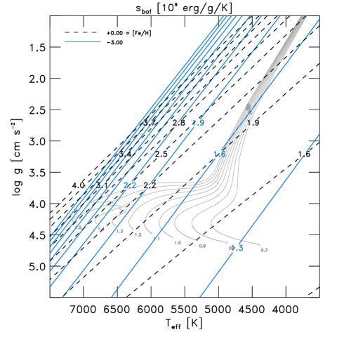
An analytical derivation of $s_{\mathrm{bot}}$ as a function of stellar parameters is rather difficult, as explained above. Nonetheless, we can fit $s_{\mathrm{bot}}$ with stellar parameter in a functional form based on the results from our simulations (see App. B). This has been done previously, based on 2D RHD models with solar metallicity by Ludwig et al. (1999). In Fig. 6, we show how $s_{\mathrm{bot}}$ varies across the Kiel diagram ($T_{\mathrm{eff}}-\log g$ diagram) for $\left[\mathrm{Fe}/\mathrm{H}\right]=0.0$ and $-3.0$. In the case of $s_{\mathrm{bot}}$, our results with solar metallicity are qualitatively in good agreement with those of Ludwig et al. (1999), despite the inherent differences between 2D and 3D convection simulations, the adopted EOS, opacities, and radiative transfer treatment. We find that $s_{\mathrm{bot}}$ (which depicts $s_{\mathrm{ad}}$) lies on lines of constant entropy in the Kiel diagram, in fact for the solar metallicity these lines with the same entropy of the adiabat run almost diagonally. Moreover, towards lower metallicity, we find two significant differences for the lines of constant $s_{\mathrm{bot}}$, the first one being that the slopes of the lines steepen, and the second being that the distances in the $T_{\mathrm{eff}}-\log g$ plane between the lines decrease. The latter implies metal-poor stars feature a broader range in $s_{\mathrm{bot}}$ compared to metal-rich ones. As we will see in Sect. 3.2, this has important consequences for the stratifications.

3.1.3 Entropy jump

The upflows enter the simulation box at the bottom with the constant entropy value of the adiabatic convection zone, $s_{\mathrm{bot}}$, and ascend until they reach the superadiabatic region (SAR) just below the visible surface, where the convective energy is converted to radiative energy. In the photosphere, the mean free path for the continuum radiation grows large enough for the gas to become transparent, and the overturning upflow at the surface loses its internal energy as photons escape and carry away entropy. Further above in the nearly isothermal atmosphere (with constant $\varepsilon$, see Fig. 16) with an exponentially decreasing density the entropy increases again due to the EOS (see Eq. 15). This leads to a minimum, $s_{\mathrm{min}}=\min\left[\left\langle s\right\rangle\right]$, just above the surface ($\log\tau_{\mathrm{Ross}}<0.0$) in the temporal and horizontal averaged entropy (see Fig. 24). We determined the entropy jump from the difference of the entropy minimum and the fixed entropy at the bottom, i.e.

$$\Delta s=s_{\mathrm{bot}}-s_{\mathrm{min}}.$$ (16)

In order to calculate $s_{\mathrm{min}}$, we used averages of the entropy on constant Rosseland optical depth, since it is the radiation losses that cause the sharp changes in the thermodynamic state around the optical surface and, therefore, the optical depth scale offers a better reference frame for comparisons. The averages on constant geometrical height $\left\langle 3\mathrm{D}\right\rangle_{z}$ smear out and thereby overestimate $s_{\mathrm{min}}$ increasingly towards higher $T_{\mathrm{eff}}$ due to the increasing level of corrugation of iso-$s$ surfaces on the geometrical scale (see Fig. 24). The constant entropy at the bottom $s_{\mathrm{bot}}$, on the other hand, is a fixed input value for each simulation. It is worthwhile to mention that the main contribution to the variation in $\Delta s$ as a function of stellar parameters is due to $s_{\mathrm{bot}}$, since $s_{\mathrm{min}}$ varies just slightly with stellar parameter compared to $s_{\mathrm{bot}}$ (see Fig. 5).

In Fig. 5 we show $s_{\mathrm{min}}$ (dashed lines) as well as $\Delta s$ (dotted lines), and it is obvious that the minimum in entropy increases just slightly with increasing $T_{\mathrm{eff}}$, while the jump increases with the constant entropy value of the adiabatic convection zone quasi-exponentially at higher $T_{\mathrm{eff}}$ and lower $\log g$. This can be concluded more easily from Fig. 18 (top panel), where we display $s_{\mathrm{bot}}$ vs. $T_{\mathrm{eff}}$ (see also Col. 8 of Table 4 and for $\Delta s$ and $s_{\mathrm{min}}$ in App. B). We note that the location of the entropy jump essentially represents the boundary of stars and the jump is to be regarded as physically realistic, which is a result of 3D RHD simulations. The entropy minimum coincides with the position of the upper end of the SAR. A similar sharp drop occurs for most of the thermodynamic quantities of interest ($\varepsilon$, $T$ and $n_{\mathrm{el}}$), whereas $\rho$ and $p_{\mathrm{tot}}$ display a marked change of gradient. Moreover, the jump in entropy is an important value, since it is a direct measure of the efficiency of convective energy transport (see Trampedach et al. 2013). The latter is in 1D modeling set by the four MLT parameters, especially $\alpha_{\mathrm{MLT}}$, in the framework of MLT (see Böhm-Vitense 1958; Henyey et al. 1965). Towards cool dwarfs $\Delta s$ becomes smaller, indicating a higher convective efficiency, while towards hotter stars the large entropy jumps reflect a low convective efficiency. We will present a calibration of $\alpha_{\mathrm{MLT}}$ based on the entropy jump in a subsequent study, as previously done by using multidimensional convection simulations (see Ludwig et al. 1999; Trampedach et al. 1999). While we found $s_{\mathrm{bot}}$ to be qualitatively similar to those of Ludwig et al. (1999), in the case of $\Delta s$ our findings are also similar, but the differences are here distinctively larger.

Figure 7: We compare the entropy jump $\Delta s$ against the constant entropy value of the adiabatic convection zone $s_{\mathrm{bot}}$ for all grid models (filled circles; color-coding explained in the legend). Furthermore, we show also hyperbolic tangent functional fits (see Eq. 35 and App. B) between $T_{\mathrm{eff}}=4000$ and $6000\,\mathrm{K}$ (red lines; top panel) and between $\log g=1.5$ and $4.5$ (grey lines; bottom panel).

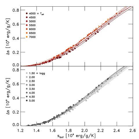
It is quite remarkable how closely the variation of $\Delta s$ resembles the change of $s_{\mathrm{bot}}$ with stellar parameters (see Fig. 5). Motivated by this, we compare directly $\Delta s$ against $s_{\mathrm{bot}}$ in Fig. 7. We find a nice correlation between $\Delta s$ vs. $s_{\mathrm{bot}}$. At lower $s_{\mathrm{bot}}$ values, $\Delta s$ seems to converge towards $0.0$ (a negative jump is not expected, since the atmosphere is losing energy in form of radiation from the photosphere), while for $s_{\mathrm{bot}}\gtrsim 1.7$, $\Delta s$ grows linearly with $s_{\mathrm{bot}}$ and only a modest level of scatter. In Fig. 7, we color-coded the $T_{\mathrm{eff}}$- and $\log g$-values respectively, to show how the residuals depend systematically on atmospheric parameters. Models with higher $T_{\mathrm{eff}}$ (bright orange dots) and higher $\log g$ (dark grey dots) settle along higher $\Delta s$ and vice versa. In order to illustrate this better, we have fitted a set of hyperbolic tangent functions (see Eq. 35), which we show also in Fig. 7. We included functional fits between $T_{\mathrm{eff}}=4000$ and $6000\,\mathrm{K}$ (red/orange lines in top panel) and between $\log g=1.5$ and $4.5$ (grey lines in bottom panel). Hence, we find hotter dwarfs along lines at larger $\Delta s$, while cooler giants settle along lines at smaller entropy jumps.

Interestingly, in the linear part ($s_{\mathrm{bot}}\gtrsim 1.7$) $\Delta s\left(s_{\mathrm{bot}}\right)$ displays a rather universal slope of $\Delta s/s_{\mathrm{bot}}\sim 0.85$, while the actual offset in the ordinate depends mainly on $T_{\mathrm{eff}}$ and $\log g$. Another interesting aspect is that $T_{\mathrm{eff}}$ shows a similar strong influence as $\log g$. The latter, however, is obviously expressed in logarithmic scale, therefore the influence of $T_{\mathrm{eff}}$ is much stronger. On the other hand, when one performs a similar hyperbolic tangent functional fit for a fixed value of $\left[\mathrm{Fe}/\mathrm{H}\right]$, then $\Delta s$ is dispersed around the functional fit with such a large scatter that a fit is rather meaningless. Therefore, in contrast to $T_{\mathrm{eff}}$ and $\log g$ we find no systematic trends with metallicity.

Based on the strong correlation between the entropy jump $\Delta s$ and $s_{\mathrm{bot}}$, it is of interest to investigate what other scaling relations may be manifested for other stellar properties. With $\Delta s$ as an inverse measure of convective efficiency, we expect that in light of such scaling relations, important quantities depending on the entropy jump will also similarly scale systematically with $s_{\mathrm{bot}}$, in particular density and velocity (see Sects. 3.2.2 and 3.2.4), and therefore also the calibrated mixing-length of a particular MLT implementation. We note briefly that qualitatively similar relations can be achieved with 1D MLT models with a fixed mixing length.

3.1.4 Emergent intensity

Figure 8: We show an overview of the emergent (bolometric) intensity for a selection of stars, namely main-sequence (MS), turnoff (TO), K-giant K-dwarf (from left to right, respectively) at a given time instant. For each star, we show four metallicities $\left[\mathrm{Fe}/\mathrm{H}\right]=0.0,-1.0,-2.0$ and $-3.0$ (from top to bottom, respectively). To facilitate comparisons between the different metallicity of each star, the intensity scale and the horizontal geometrical size of the metal-poor simulations are identical to $\left[\mathrm{Fe}/\mathrm{H}\right]=0.0$, and the individual intensity contrasts $\left[\%\right]$ are indicated in each box.

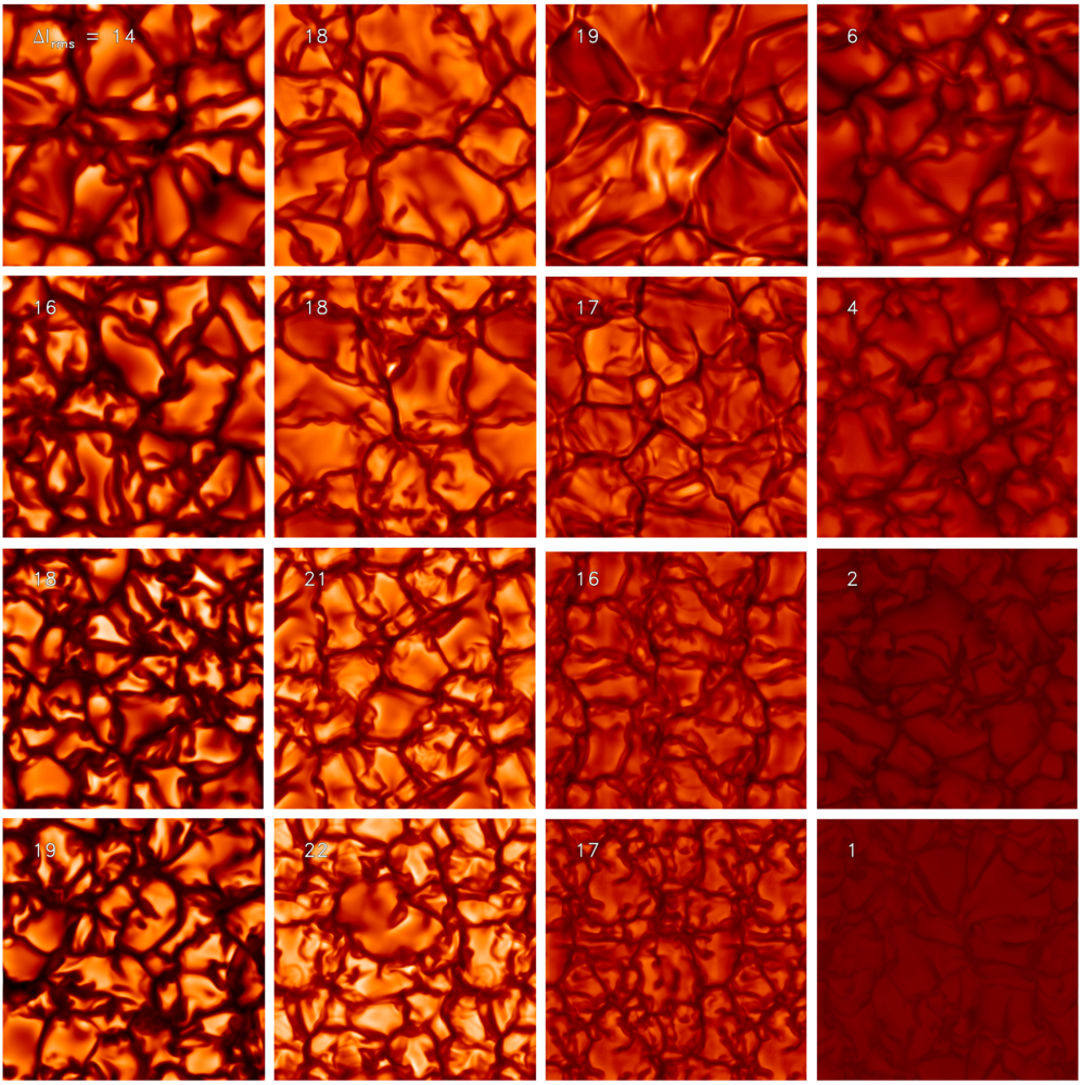
While classic 1D models are inherently horizontally symmetric, therefore lacking a visible granulation pattern, the emergent intensity of 3D models features inhomogeneities exhibiting rich details, which arise due to the presence of turbulent convective motions. We give an overview the emergent intensity of our simulations in Fig. 8. Therein we display a main-sequence (MS) simulation (the Sun), a turnoff (TO) simulation, a K-giant, and a K-dwarf model, each with four different metallicities. To facilitate direct comparisons among the four metallicities, we kept the horizontal sizes and the color scales for the continuum intensities fixed from $\left[\mathrm{Fe}/\mathrm{H}\right]=0.0$ for the individual stellar categories (we extended the metal-poor simulations by exploiting the periodic horizontal boundary conditions). The dark regions depict the cold intergranular lanes, while the brighter areas are the hot granules. The radiation above the granules originate at higher geometrical heights, while for downdrafts it comes from much lower heights. This is because the opacity is highly nonlinear due to the strong temperature sensitivity of the $\mathrm{H}^{-}$-opacity ($\kappa_{\mathrm{H}^{-}}\sim T^{10}$, see SN98), which is the by far the dominant continuum opacity source in the visible for late-type stellar photospheres. Since the temperature difference between the granules and the intergranular lanes is very large ($>10^{3}\,\mathrm{K}$), layers of constant optical depth will be increasingly more corrugated and become largest around the peak of the SAR. Therefore, the radiation above granules is emerging from higher geometrical depths, $z_{\mathrm{up}}$, while above downdrafts it originates from deeper geometrical heights, $z_{\mathrm{dn}}$ (for the Sun the largest difference between the averaged geometrical heights can amount up to $\left\langle z\right\rangle_{\mathrm{up}}-\left\langle z\right\rangle_{\mathrm{dn}}\simeq-140\,\mathrm{km}$ at $\log\tau_{\mathrm{Ross}}=2.0$).

An immediate, interesting aspect that leaps to the eye from the overview presented in Fig. 8 is the qualitative self-similarity of the granulation patterns despite the large variations in size-scales. The emergent intensity increases towards higher $T_{\mathrm{eff}}$ and decreases for lower surface gravities, as expected. From Fig. 8, it is also clear that the granule sizes decrease with metallicity (due to smaller $H_{P}$, see Sect. 3.1.5; see also Collet et al. 2007). Also apparent is the change of intensity contrast with stellar parameters, as we will discuss below.

Figure 9: We show the temporally averaged histograms of the (bolometric) intensity (solid lines) for various stellar parameters (the bin-size is 100). To ease comparisons between the different stellar parameters, we normalized the individual intensity scales with its mean value. Furthermore, we have indicated the respective FWHM of the intensity histograms, $I_{\mathrm{FWHM}}$, (dotted lines), a measure of the intensity contrast. Note the different ordinate scale in the top panel. The bimodal distributions are given due to the asymmetry and the large contrast in the up and downflows.

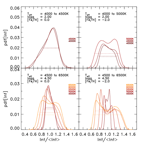
In order to discuss the changes in the intensity, we show in Fig. 9 the temporally averaged histograms of the intensity $I$ normalized to their individual mean intensity $\overline{I}$, thereby enabling a direct comparison between different stellar parameters. The histograms of the intensity show two components: a peak at lower (darker, $I/\overline{I}<1.0$) intensities, resulting from the cool downdrafts, and an often broader component at higher (brighter, $I/\overline{I}>1.0$) intensities, arising from the upflowing hot granules. We note that these findings are qualitatively to be expected (see SN98; Trampedach et al. 2013).

As clearly depicted in Fig. 9, the shapes of the two components change with stellar parameters, in particular the amplitudes and widths, thereby changing the overall shape. The two components can be clearly extracted from histograms at higher $T_{\mathrm{eff}}$, where the intensity contrast is increasingly enhanced and eventually produces a distinctly bimodal distribution, which is a manifestation of the hidden or naked granulation (see Fig. 10 and Nordlund & Dravins 1990). In order to better illustrate this, we also included the full width at half maxima (FWHM) of the individual intensity histograms $I_{\mathrm{FWHM}}$ in Fig. 10. On the other hand, at lower $T_{\mathrm{eff}}$ the intensity contrast decreases in general, so that the two components overlap, leading to a single narrower higher peak in the histogram, thereby becoming indistinguishable from each other in the histogram. Ludwig & Kučinskas (2012) found also an unimodal intensity distribution in the context of a 3D giant model with solar metallicity. Furthermore, we find that the individual contribution to the intensity from upflows and downflows is often asymmetric, meaning that the amplitudes of the two peaks in the bimodal distribution are unequal (see Fig. 9). In general, for dwarfs, we find that the relative importance of downflows with respect to upflows in terms of the peak contribution to the intensity distribution increases with increasing $T_{\mathrm{eff}}$. However, we also find exceptions, e.g. at lower metallicity where the behavior at $T_{\mathrm{eff}}=4500\,\mathrm{K}$ is actually the opposite. Also, the balance between upflows and downflows varies with surface gravity. The intensity histograms for giants are in general broader (higher contrast) compared to dwarfs of the same $T_{\mathrm{eff}}$ (see $I_{\mathrm{FWHM}}$), hence exhibiting a larger intensity contrast. For dwarfs at lower metallicity (right bottom panel) the bimodality is more pronounced and the $I_{\mathrm{FWHM}}$ (contrast) is broader (higher) towards higher $T_{\mathrm{eff}}$, while at lower $T_{\mathrm{eff}}$ the $I_{\mathrm{FWHM}}$ (contrast) becomes narrower (lower) compared to solar metallicity (left bottom panel). The latter hints at an enhancement of the effect of hidden or naked granulation.

Figure 10: Overview of the (bolometric) intensity contrast $\Delta I_{\mathrm{rms}}$ against $T_{\mathrm{eff}}$ for $\left[\mathrm{Fe}/\mathrm{H}\right]=-2.0$ and $0.0$ (blue and black respectively). Models with the same gravity, but different $T_{\mathrm{eff}}$ are connected. The enhanced naked or hidden granulation at lower metallicity can be extracted in the larger range of intensity contrasts (see text for details).

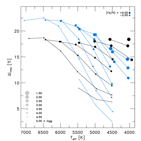
To illustrate the latter in more detail, we show in Fig. 10 the rms of the bolometric disk center intensity fluctuations for $\left[\mathrm{Fe}/\mathrm{H}\right]=0.0$ and $-2.0$, which is commonly referred as the intensity contrast

$$\Delta I_{\mathrm{rms}} = \left[\sum\left(I_{i}-\overline{I}\right)^{2}/N\overline{I}^{2}\right]^{1/2}$$ (17)

with $\overline{I}$ being the (spatial) mean intensity and $N$ the number of data points (see Roudier & Muller 1986). We remark that the shown $\Delta I_{\mathrm{rms}}$ are is temporal averages. It is essentially defined as the relative standard deviation, hence it reflects the width of the intensity distribution (see Fig. 9). This often measured value is very suitable for quantifying the range of brightness fluctuations due to granulation. The intensity contrast increases with higher $T_{\mathrm{eff}}$ and lower $\log g$. For our solar simulation we get an intensity contrast of $15\,\%$, which is close to the one found by SN98 with $16\,\%$ (see Col. 10 in Table 4).

Towards higher $T_{\mathrm{eff}}$, we find that $s_{\mathrm{bot}}$, $\Delta s$, and the vertical velocity increase, as shown in Sects. 3.1.2 and 3.2.2. For increasingly hotter stars, the top of the convective zone, $z_{\mathrm{top,cz}}$, penetrates higher and higher above the optical surface due to larger vertical velocities (see Fig. 17). Additionally, at higher $T_{\mathrm{eff}}$ (higher $s_{\mathrm{bot}}$ and $\Delta s$), the overall temperatures and their fluctuations also increase, implying that one observes increasingly higher layers, since the dominant $\mathrm{H}^{-}$-opacity, hence the optical depth, depends sensitively on the temperature. Therefore, the granulation pattern is enhanced at higher $T_{\mathrm{eff}}$, while on the contrary for lower $T_{\mathrm{eff}}$ the granulation becomes less visible, since $z_{\mathrm{top,cz}}$ recedes below the optical surface in the latter case (see overview in Fig. 8). This phenomenon has been already described by Nordlund & Dravins (1990) as naked granulation.

Interestingly, in our simulations, we find that at lower metallicity the effect of naked and hidden granulation is more pronounced, in the sense that the range of contrast from cool, low-contrast dwarfs, to hotter, high-contrast dwarfs, is $61\,\%$ larger (from $10.9$ to $17.6$) for our $\left[\mathrm{Fe}/\mathrm{H}\right]=-2.0$ simulations than for solar metallicity (see Fig. 10). At lower metallicity the major electron donors (metals) are depleted, therefore the formation of the dominant opacity source $\mathrm{H}^{-}$ depends primarily on the ionization of hydrogen, which is the reason for the steep increase of intensity contrast with for higher $T_{\mathrm{eff}}$ (Nordlund & Dravins 1990).

The variations in the intensity and in the intensity contrast with stellar parameters have important ramifications for observations. At the one hand, the enhanced naked or hidden granulation at lower metallicity affects the formation of spectral lines and the limb darkening. On the other hand, it should also lead to distinct signatures in the granulation background of asteroseismological observations and spectro-interferometric imaging. Here, we limit ourselves to the discussion of the global properties of the emergent intensity patterns, and a detailed analysis will be performed in subsequent papers.

3.1.5 Granule size

Figure 11: Overview of the granule diameter $d_{\mathrm{gran}}$ derived from the maximum of the mean 2D spatial power spectrum of the bolometric intensity against $T_{\mathrm{eff}}$ for $\left[\mathrm{Fe}/\mathrm{H}\right]=-2.0$ and $0.0$ (blue and black respectively). Models with the same gravity are connected by their respective functional fits (solid lines; see App. B).

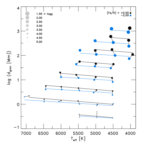
The physical dimensions of the simulations boxes ($s_{x},s_{y}$ and $s_{z}$ in Cols. 11 and 12 of Table 4) are selected based on the mean diameter of granules (see Sect. 2.3.1 and Table 4) and a target of about 10 granules in the box. Additionally, we measured the granule sizes by calculating the 2D spatial power spectrum of the bolometric intensity for the time series, and determining its maximum from the smoothed time average (see Fig. 9 in Trampedach et al. 2013). This method is quite robust despite the large variations in gravity. In Fig. 11, we present the measured granule sizes $d_{\mathrm{gran}}$ (given in Col. 13 in Table 4; see also App. B), showing that they become larger with smaller surface gravity. Also, the granules of the simulations with fixed $\log g$, the lowest $T_{\mathrm{eff}}$ are typically $\sim 50\,\%$ smaller compared to the simulations with the hottest $T_{\mathrm{eff}}$, while for the models with the lowest metallicity they are typically $\sim 30\,\%$ smaller than for the metal-rich ones.

Figure 12: In the top panel, we compare the granule size approximated with the pressure scale height $d_{\mathrm{NIC}}$ (see Eq. 18) against the mean granule diameter $d_{\mathrm{gran}}$ (same as Fig. 11) for all models. The individual stellar parameters are indicated ($T_{\mathrm{eff}}$, $\log g$ and $\left[\mathrm{Fe}/\mathrm{H}\right]$ with red, gray, and blue respectively). We indicated the position of $d_{\mathrm{NIC}}=d_{\mathrm{gran}}$ the solid diagonal line. In the bottom panel, we show also the relative residuals. We indicated also the mean residual (dotted line), which amounts to $\sim 30\,\%$. Here, models with the same gravity are connected (solid grey lines).

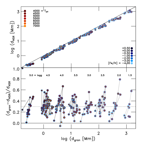
We find a remarkable validation for the approximation of the maximal horizontal extent of a granule based on mass-conservation considerations made by SN98 (see also Nordlund et al. 2009). Hereafter, we denote the following relation as the Nordlund scaling relation (NSR). The ascending buoyant plasma inside a cylindrical granule with radius $r$ gives rise to a vertical mass flux with $j_{z}=[\pi r^{2}]\rho v_{z}$. This mass flux has to deflect and overturn increasingly towards the top. Due to conservation of mass, the upflow has to drain off sideways through the edge of the granule within approximately one pressure scale height $H_{P}$, hence resulting in a horizontal mass flux $j_{h}=[2\pi rH_{P}]\rho v_{h}$. The pressure is a quantity that preserves its characteristic shape with stellar parameters, i.e. the pressure of two different simulations look rather similar on a uniform depth scale, therefore the pressure scale height is preferred over the density scale height. Equating $j_{z}$ and $j_{h}$ we can solve for the (maximal) granular diameter, $d=2r$:

$$d_{\mathrm{NSR}} = 4\left[v_{h}/v_{z}\right]H_{P}\approx 4H_{P}$$ (18)

We show in Fig. 12 a comparison of the granular diameters estimated with $d_{\mathrm{NIC}}$ and from the maximum of 2D spatial power spectra $d_{\mathrm{gran}}$, which is shown in Fig. 11. The astonishing tight correlation can solely be interpreted as clear evidence for the validity of the NSR. We find that the mean pressure scale height taken at the height of the maximum vertical rms-velocity below the optical surface ($\log\tau_{\mathrm{Ross}}\sim 2.0$, see Fig. 17) gives the best match between $d_{\mathrm{NIC}}$ and the granule sizes. Furthermore, we also confirm that the relevant scale-height is that of the total pressure scale height, $H_{P}=p_{\mathrm{tot}}/\rho g$, since we find a better agreement with the latter. The granular diameters found from the peak of 2D spatial power spectra are about $30\,\%$ larger than the estimate from Eq. 18, i.e., $d_{\mathrm{gran}}\sim 1.3d_{\mathrm{NIC}}$ (see lower panel of Fig. 12). The variation of the velocity ratio $v_{h}/v_{z}$ in the convection zone is rather small ($v_{h}/v_{z}$$\sim 1.0$) as both are of the order of the sound speed, therefore the variation in Eq. 18 stems predominantly from $H_{P}$. In hydrostatic equilibrium the pressure scale height is inversely proportional to the surface gravity ($H_{P}\propto 1/g$), which explains the strong correlation between the granular sizes and $\log g$. On the other hand, with increasing $T_{\mathrm{eff}}$ and $\left[\mathrm{Fe}/\mathrm{H}\right]$, the pressure scale height increases slightly because of the increase in the ratio of pressure and density ($H_{P}\propto p_{\mathrm{tot}}/\rho$). The ratio actually increases even though both values decrease, since the density drops with height slightly more rapidly than the pressure.

Finally, we want to mention our finding on the filling factor for upflows and downflows, $f_{\mathrm{up}}$ and $f_{\mathrm{dn}}$ respectively. We derived the filling factor from the sign of the velocity field in the unaltered simulations on layers of constant geometrical height. Then we computed the mean filling factor in the convection zone, which yields on average for all simulations $f_{\mathrm{up}}\simeq 0.65$ with a minute deviation of $\sigma=0.014$. Therefore, we find that the mean filling factor is rather universal, and close to previous findings by SN98 with $f_{\mathrm{up}}\sim 2/3$ and $f_{\mathrm{dn}}\sim 1/3$. In deeper solar simulations, which reach down to $20\,\mathrm{Mm}$ (Stein et al. 2011), we find very similar values for the filling factor.

3.2 The mean atmosphere

In the following, we want to discuss the properties of the mean stratifications and the temporal and spatial averages of various important quantities. Unless specified otherwise, the $\left\langle 3\mathrm{D}\right\rangle$ stratifications presented here are averages on surfaces of constant Rosseland optical depth, i.e. $\left\langle 3\mathrm{D}\right\rangle=\left\langle 3\mathrm{D}\right\rangle_{\mathrm{Ross}}$. Whenever we employ alternative averages in the text, e.g., on constant geometrical height $\left\langle 3\mathrm{D}\right\rangle_{z}$, we indicate that explicitly. We remark briefly that only the averages on constant geometrical height $\left\langle 3\mathrm{D}\right\rangle_{z}$ strictly fulfill the equations of conservation (Eqs. 1, 2 and 3), therefore also the hydrostatic equilibrium, while all other averages exhibit slight deviations. This and the actual methods we used to compute the mean stratifications are discussed in a separate paper (see Magic et al. in preparation). For the sake of clarity, we display here only a subsample of our grid models including MS and RGB stars ($\log g=4.5$ and $2.0$, which we refer to as dwarfs and giants, respectively) with solar and sub-solar metallicity ($\left[\mathrm{Fe}/\mathrm{H}\right]=0.0$ and $-2.0$, solar and metal-poor, respectively). Whenever possible, we compare with corresponding 1D models that are obtained with our 1D code (see App. A).

Before continuing our discussion, we would like to point out the importance of the superadiabatic region (SAR), as it will be referred repeatedly in the following. It is the region, where the transport of energy changes character, from convective to radiative. The top of the SAR, where $\@vec{\nabla}_{\mathrm{sad}}=0$, marks the top the convection zone, since it is the uppermost point, where the Schwarzschild criterion is fulfilled. At the location of the peak of the superadiabatic gradient, one also finds the largest fluctuations and inhomogeneities in the thermodynamic variables due to the non-adiabatic transition to the photosphere. Furthermore, it is here in the SAR, where the entropy jump and the peak in the vertical velocity occur. In fact, the SAR effectively represents the physical outer boundary of the convective envelope. It is the most dynamic part in the interior of late-type stars, where the largest fluctuations are found. This is the reason why hydrostatic 1D modeling has the greatest challenges in this rather small region.

3.2.1 Temperature stratification

Figure 13: $\left\langle 3\mathrm{D}\right\rangle$ stratifications of the temperature vs. optical depth for various stellar parameters (solid lines) and 1D models with $\alpha_{\mathrm{MLT}}=1.5$ (dashed lines). Furthermore, we have marked the positions of entropy minimum (plus), vertical peak velocity (diamond), and maximum in $\nabla_{\mathrm{sad}}=\nabla-\nabla_{\mathrm{ad}}$ (triangle).

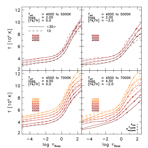
We first consider the temperature stratifications in optical depth, which we show in Fig. 13. We also show the corresponding stratifications of 1D theoretical model atmosphere with $\alpha_{\mathrm{MLT}}=1.5$ based on our 1D code (dotted lines) with identical EOS and opacity tables as the 3D models. In the continuum forming layers around the optical surface ($-1.0<\log\tau_{\mathrm{Ross}}<0.5$), the differences between $\left\langle 3\mathrm{D}\right\rangle$ models with different $T_{\mathrm{eff}}$s, but same $\log g$ and $\left[\mathrm{Fe}/\mathrm{H}\right]$, are rather small besides the shift in the temperature stratification corresponding to the difference in effective temperature $\Delta T_{\mathrm{eff}}$, which is to be expected since $T_{\mathrm{eff}}\approx T\left(\tau=2/3\right)$. Well above and below the optical surface, on the other hand, we find significant differences between the $\left\langle\mathrm{3D}\right\rangle$ models depending on the stellar parameters.

In the upper layers ($\log\tau_{\mathrm{Ross}}<-2.0$) of atmospheres with solar metallicity, we find that the behavior in mean temperature is similar between 3D and 1D models. On the other hand, the metal-poor $\left\langle\mathrm{3D}\right\rangle$ models exhibit significantly cooler temperature stratifications compared to $\left\langle\mathrm{3D}\right\rangle$ models with solar metallicity ($\Delta T/T\left(\log\tau_{\mathrm{Ross}}=-0.5\right)\sim-1\%$ and $\sim-14\%$ for $\left[\mathrm{Fe}/\mathrm{H}\right]=-1.0$ and $-3.0$ respectively), in particular for dwarfs ($\log g=4.5$). The temperature stratification in the upper photospheres of solar-metallicity models is largely controlled by radiative equilibrium, while for low-metallicity models this is not generally the case: for metal-poor models, the absorption features become considerably weaker, therefore, the radiative heating by spectral line re-absorption ($q_{\mathrm{rad}}$) is dominated by the adiabatic cooling due to expansion of the ascending gas ($-p_{\mathrm{th}}\@vec{\nabla}\cdot\@vec{v}$) in the energy balance (Eq. 3), leading to an equilibrium structure at cooler temperatures (Asplund et al. 1999b). For cool, metal-poor giants (e.g., $T_{\mathrm{eff}}=4000\,\mathrm{K}$, $\log g=2.0$), we recognize the effects of molecule formation on the structure of the high atmosphere. At sufficiently low temperatures, molecules start to form, which contribute with a large line opacity, shifting the balance from adiabatic to radiative heating and cooling, resulting in a stratification closer to the radiative equilibrium one (see Gustafsson et al. 2008). On the other hand, for giants with solar metallicity the radiative equilibrium is even more dominating, since these exhibit hotter stratifications than 1D models in the upper layers. Ludwig & Kučinskas (2012) find the same but on a much milder level. These effects are rather non-linear, and we find no simple systematic trends within our grid models.

Figure 14: $\left\langle 3\mathrm{D}\right\rangle$ temperature stratifications with the variation of one stellar parameter at a time, while the two others are fixed ($T_{\mathrm{eff}}$, $\log g$, and $\left[\mathrm{Fe}/\mathrm{H}\right]$, from top to bottom, respectively). We show our standard averages on constant optical depth $\left\langle 3\mathrm{D}\right\rangle$ (solid line) and on constant geometrical depth $\left\langle 3\mathrm{D}\right\rangle_{z}$ (dotted line).

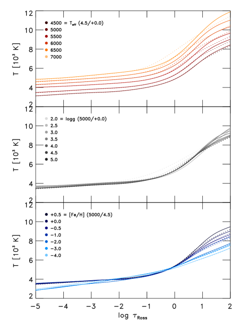
We would now like to examine the influence of individual stellar parameters on the temperature stratification. Therefore, we show in Fig. 14 the temperature stratifications of models where we separately vary one at the time ($T_{\mathrm{eff}}$, $\log g$, and $\left[\mathrm{Fe}/\mathrm{H}\right]$), while keeping the other two parameters constant. Figure 14 (top panel) shows, as expected, that with increasing $T_{\mathrm{eff}}$, the temperature stratification becomes overall hotter above, but also below the optical surface, in order to provide the required total energy flux (higher enthalpy, Eq. 22). We find in our simulations (both 1D and 3D) that the increased $T_{\mathrm{eff}}$s with hotter stratifications are accompanied by lower densities and higher vertical velocities below the surface (see $p_{\mathrm{tot}}\left(\log\tau_{\mathrm{Ross}}=2.0\right)$ in Fig. 22 representatively for the $\rho$). The net effect on the convective flows are lower mass fluxes for higher $T_{\mathrm{eff}}$s, since the decrease in density is predominating the increase in velocity, therefore resulting in a more inefficient convection. This is compensated with higher entropy jumps (see Fig. 18 with $\Delta s$ as an inverse measure for convective efficiency), hence higher temperatures and steeper temperature gradients. On the other hand, the temperatures in the upper, radiative layers increase less with increasing $T_{\mathrm{eff}}$ than in the deeper, convective ones. We find with decreasing surface gravity (middle panel in Fig. 14) the same correlations as with increasing $T_{\mathrm{eff}}$s before, the temperature stratifications become hotter below the photosphere, and due to lower densities we find a more inefficient convection, while the upper atmosphere is less affected. For lower metallicities (bottom panel), the temperature stratifications are significantly cooler, both above and below the optical surface ($\Delta T/T\left(\log\tau_{\mathrm{Ross}}=2.0\right)\sim-5\%$ and $-15\%$ for $\left[\mathrm{Fe}/\mathrm{H}\right]=-1.0$ and $-3.0$ respectively). At the top the stratifications are cooler at lower $\left[\mathrm{Fe}/\mathrm{H}\right]$ due to the dominance of adiabatic cooling over radiative heating. Below the optical surface, we find higher densities with lower velocities and entropy jumps (while the mass flux is increasing), therefore, leading to an efficient convection with shallow temperature gradients at lower metallicities. We find cooler models that fall below the opacity edge, which we describe below (compare $T_{\mathrm{eff}}=5000\,\mathrm{K}$ in Fig. 16), follow an adiabatic temperature stratification even in the atmosphere, which coincides with the rather sudden change between $\left[\mathrm{Fe}/\mathrm{H}\right]=-1.0$ and $-2.0$ in Fig. 14 (bottom panel). Besides our standard averages on constant Rosseland optical depth, we show also the averages on constant geometrical depth scale $\left\langle 3\mathrm{D}\right\rangle_{z}$ (here is $z$ fixed and $\tau_{\mathrm{Ross}}=\left\langle\tau_{\mathrm{Ross}}\right\rangle_{z}$), which are systematically different, in particular below the optical surface, but behave qualitatively in a similar way with stellar parameters.

Figure 15: Overview of the maximum temperature gradient $\nabla_{\mathrm{peak}}$ (top panel) and Rosseland opacity $\kappa_{\mathrm{Ross}}$ taken at the height $\tau_{\mathrm{Ross}}\approx 3.0$ (bottom panel) against $T_{\mathrm{eff}}$ for $\left[\mathrm{Fe}/\mathrm{H}\right]=-2.0$ and $0.0$ (blue and black respectively). Models with the same surface gravity are connected by their respective functional fits in the top panel (solid lines; see App. B).

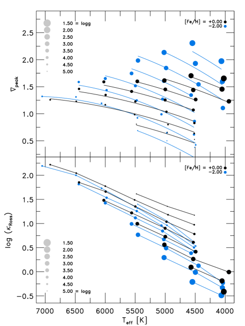
In the sub-photospheric region ($\log\tau_{\mathrm{Ross}}>0.5$), where convection dominates, the temperature gradients $\nabla=d\ln T/d\ln p_{\mathrm{tot}}$ become increasingly steeper with higher $T_{\mathrm{eff}}$, reflecting the hotter interior stratifications. This can be illustrated with the maximum in temperature gradient, $\nabla_{\mathrm{peak}}=\max\nabla$, which we show in Fig. 15 (functional fits are also given in App. B). The increase of $\nabla_{\mathrm{peak}}$ with $T_{\mathrm{eff}}$ is close to linear, but it seems to saturate at higher $T_{\mathrm{eff}}$ (see $T_{\mathrm{eff}}\geq 6500\,\mathrm{K}$). We find that the maximum in temperature gradient $\nabla_{\mathrm{peak}}$ reproduces qualitatively a similar behavior as the intensity contrast $\Delta I_{\mathrm{rms}}$ with stellar parameter (compare Figs. 10 and 15), which is consistent with the strong temperature sensitivity of the $\mathrm{H}^{-}$ opacity. Furthermore, our metal-poor simulations exhibit a larger range of $\nabla_{\mathrm{peak}}$-values than their solar metallicity counterparts, and $\nabla_{\mathrm{peak}}$ is similarly enhanced at lower metallicity (compare also $T\left(\log\tau_{\mathrm{Ross}}=2.0\right)$ for dwarfs in Fig. 13), as the intensity contrast (see Sect. 3.1.4). Our cool metal-poor simulations have flatter and hot metal-poor simulations have steeper temperature stratifications than the metal-rich part of our grid (see Fig. 14). Curiously, $\nabla_{\mathrm{peak}}$ is close to constant with metallicity for the solar $T_{\mathrm{eff}}$ and $\log g$.

We identify three main reasons for the given variations in temperature gradients with stellar parameters in the SAR, which are rooted in the hydrodynamics and the radiative transfer: velocity field, convective efficiency, and radiative back-warming.

1. As we discussed above (see Sect. 3.1.3), the entropy jump $\Delta s$ increases with effective temperature according to a power law (see Fig. 18). This behavior arises due to the variations in the radiative losses (see Sect. 3.2.8), which is accompanied by changes in internal energy and density (see Fig. 16). The velocities rise rapidly, as exhibited by the growth of $v_{z,\mathrm{rms}}^{\mathrm{peak}}$ and also $p_{\mathrm{turb}}^{\mathrm{peak}}$ with $T_{\mathrm{eff}}$ (see Figs. 17 and 21 respectively). Similar to $\nabla_{\mathrm{peak}}$, both $v_{z,\mathrm{rms}}^{\mathrm{peak}}$ and $p_{\mathrm{turb}}^{\mathrm{peak}}$ occur in the SAR, and both increase towards higher $T_{\mathrm{eff}}$ and lower $\log g$.

2. The mass mixing length $\alpha_{m}$ changes with stellar parameters (Trampedach & Stein 2011). The latter is evaluated as the inverse gradient of the vertical mass flux, separately in the up- or downflows, hence $\alpha_{m}^{-1}=d\ln j_{z,\mathrm{up}}/d\ln p$, with $j_{z,\mathrm{up}}$ being the vertical mass flux in the upflows. Therefore, the mass mixing length is composed of the gradients of the density and the vertical velocity, i.e. $\alpha_{m}\propto 1/d\ln\rho+1/d\ln v_{z}$. We find that $\alpha_{m}$ increases for lower $\Delta s$, $v_{z,\mathrm{rms}}^{\mathrm{peak}}$ and $\nabla_{\mathrm{peak}}$. We will publish our findings on the mass mixing length in a separate paper.

3. In the lower photospheric layers, where the continuum forms, radiation is absorbed (blocked) by spectral lines; this implies that less radiative flux can be transported at the wavelengths corresponding to spectral lines and, conversely, that more flux has to be pushed through continuum windows, an effect commonly referred to as line-blanketing. This in turn leads to a steepening of the temperature gradient and to additional heating of the sub-surface layers, also known as back-warming (see Mihalas 1970; Nordlund et al. 2009). In 1D models it is straightforward to quantify the effect of back-warming, as done for example by Gustafsson et al. (2008), who found it to contribute a slight increase in temperatures below the surface ($\Delta T/T\left(\tau_{\mathrm{Ross}}=10\right)\simeq 5\%$ for solar metallicity stars with $T_{\mathrm{eff}}\approx 5000\,\mathrm{K}$ and $\log g=3.0$). In our 3D RHD atmosphere models, line-blanketing and back-warming effects are also naturally included through our opacity-binning method. Isolating the radiative back-warming effect in our 3D simulations is, however, a little more involved than in 1D and we defer the analysis of this mechanism to a future paper in this series.

The three mentioned effects are nonlinearly coupled and compete with each other, making it difficult to disentangle the individual contributions. A quantitative analysis will be presented in a later paper.

Figure 16: We show the mean internal energy against mean density for dwarf models ($\log g=4.5$) with $\left[\mathrm{Fe}/\mathrm{H}\right]=0.0$ and $-2.0$ (left and right respectively). The specific isocontours for the entropy $s_{\mathrm{bot}}$ (green solid) and $s_{\mathrm{min}}$ (green dotted), Rosseland opacity per volume, $\rho\kappa_{\mathrm{Ross}}$, (blue) and temperature $T$ (orange) are underlayed. Moreover, the positions of entropy minimum $s_{\mathrm{min}}$ (plus), optical surface (large square), vertical peak velocity $v_{z,\mathrm{rms}}^{\mathrm{peak}}$ (diamonds) and maximum in $\nabla_{\mathrm{sad}}$ (triangle) are marked respectively. The amplitude of $v_{z,\mathrm{rms}}^{\mathrm{peak}}$ is indicated with horizontal bars with markings in 1 km/s. We also included the 1D models with $\alpha_{\mathrm{MLT}}=1.5$ (blue dashed lines). The range in optical depth is shown from $\log\tau_{\mathrm{Ross}}=-5.0$ to $+5.0$ for each dex (small squares). However, we note that our simulations boxes are much deeper ($\left\langle\log\tau_{\mathrm{Ross}}\right\rangle\approx+7.5$).

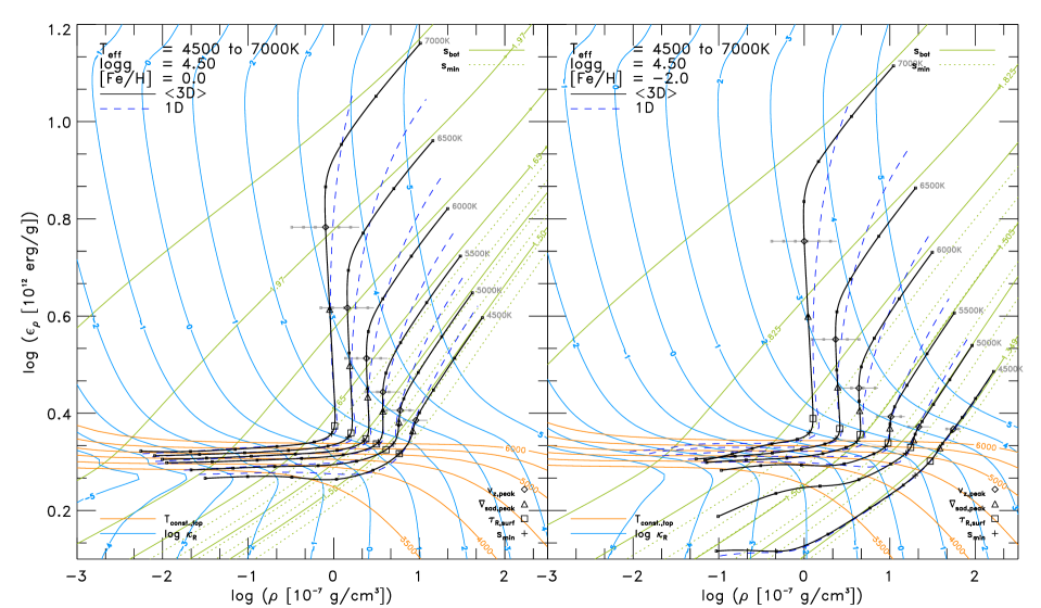
We would like now to examine more closely a sample of $\left\langle 3\mathrm{D}\right\rangle$ models in the $\varepsilon-\rho$-plane, as shown in Fig. 16, in order to better illustrate the variations with stellar parameters. One can clearly distinguish three different regimes: the adiabatic convection zone, the photospheric transition, and the almost isothermal upper atmosphere.

At the bottom boundary, sufficiently deep in the convection zone where entropy fluctuations become small, $\left\langle\delta s\right\rangle=0.3\,\%$, the models follow closely the associated adiabats with $s=s_{\mathrm{bot}}$ (green lines). They deviate increasingly from their adiabats, as the top of the convection zone is approached. This is due to the entropy deficient downdrafts (cooled in the photosphere) becoming less diluted by the entropic upflows, as the optical surface is approached. For the 1D models (blue dashed lines), the value of the entropy at the bottom of the stratifications is evidently overestimated, particularly at higher $T_{\mathrm{eff}}$, but this is because we haven’t calibrated the $\alpha_{\mathrm{MLT}}$ parameter here, and we have used a value of $1.5$ for all models. The transition of energy transport from fully convective to fully radiative is clearly visible, since, at the optical surface, one finds a sharp isochoric ($\Delta\rho\sim 0.0$) drop in internal energy (this is basically the enthalpy-jump $\Delta h$ in Eq. 22). The $\varepsilon$-jump coincides with the sub-photospheric region ($0.0<\log\tau_{\mathrm{Ross}}<2.0$), where the atmosphere starts to become transparent. The transition zone ends eventually at the optical surface ($\log\tau_{\mathrm{Ross}}\simeq 0.0$, marked with big squares). Above the optical surface ($\log\tau_{\mathrm{Ross}}<0.0$) the atmosphere is almost isothermal (compare with the orange isotherms in Fig. 16), with exponentially decreasing density and almost constant internal energy ($\Delta\varepsilon\sim 0.0$).

The entropy $s_{\mathrm{bot}}$ at the bottom grows exponentially with increasing $T_{\mathrm{eff}}$ and decreasing $\log g$. We showed above that the entropy jump increases in a similar way (see Fig. 7). Here we find a similar behavior for the jump in internal energy ($\Delta\varepsilon$, hence $\Delta h$) in the photosphere. Moreover, we show in Fig. 16 the positions of $\nabla_{\mathrm{sad}}^{\mathrm{peak}}$ and $v_{z,\mathrm{rms}}^{\mathrm{peak}}$ located in the $\varepsilon$-jump, and, again, we find both $v_{z,\mathrm{rms}}^{\mathrm{peak}}$ and $\nabla_{\mathrm{sad}}^{\mathrm{peak}}$ to scale exponentially with $T_{\mathrm{eff}}$. For $v_{z,\mathrm{rms}}^{\mathrm{peak}}$ we have indicated the amplitudes as well, which also increases exponentially with $T_{\mathrm{eff}}$. All of the aforementioned positions are distributed rather regularly in the $\varepsilon-\rho$-plane, while they are less so on the $\log\tau_{\mathrm{Ross}}$-scale (see Fig. 13). The position of $s_{\mathrm{min}}$ is close to the optical surface and shows little variation in optical depth.

At lower energies and densities in Fig. 16 ($\log\varepsilon\sim 0.3$ and $\log\rho\sim 3.0$ to $0.0$) we notice the effect of H i and He i opacity in form of an edge in the opacity contours ($\log\kappa_{\mathrm{Ross}}\sim-5.0$ to $-1.0$), since the bound-free absorption increases (more excited states) towards higher energy below the ionization energy, and they fade away again above it. Models that fall below this edge exhibit a rather different stratification. In particular, towards cool metal-poor dwarfs, i.e. lower $T_{\mathrm{eff}}$, higher $\log g$, and lower $\left[\mathrm{Fe}/\mathrm{H}\right]$, the models more closely follow adiabats than isotherms, in the atmosphere. This effect of the competition between radiative and dynamic heating (see beginning of this Sect.) above the convection zone becomes particularly evident at lower metallicity (for $\left[\mathrm{Fe}/\mathrm{H}\right]\leq-2.0$). However, for the 1D models (blue dashed lines), this is obviously not the case, since these always follow isotherms due to the enforcement of radiative equilibrium. Furthermore, the cool metal-poor $\left\langle 3\mathrm{D}\right\rangle$ models also display higher densities at the optical surface, thereby spanning a larger $\rho$-range for different $T_{\mathrm{eff}}$s. The stratifications of simulations of hotter dwarfs, on the other hand, depend little on metallicity. For the simulations, we have only plotted the range $\log\tau_{\mathrm{Ross}}\in\left[-5.0,5.0\right]$, and the top of this is reached at much higher densities for the metal-poor dwarfs than for the solar metallicity dwarfs. Therefore, the density ranges covered above the optical surface by the individual atmospheres is small for metal-poor models ($\min\left[\log\rho\right]\sim-1.0$ and $-2.0$, respectively; see Fig. 16).

3.2.2 Velocity field

Figure 17: Vertical rms-velocity, $v_{z,\mathrm{rms}}$, from the $\left\langle 3\mathrm{D}\right\rangle$ stratifications (solid lines) and convective velocity $v_{\mathrm{MLT}}$ from the corresponding 1D MLT models (dotted lines) as function of optical depth $\log\tau_{\mathrm{Ross}}$ for various stellar parameters.

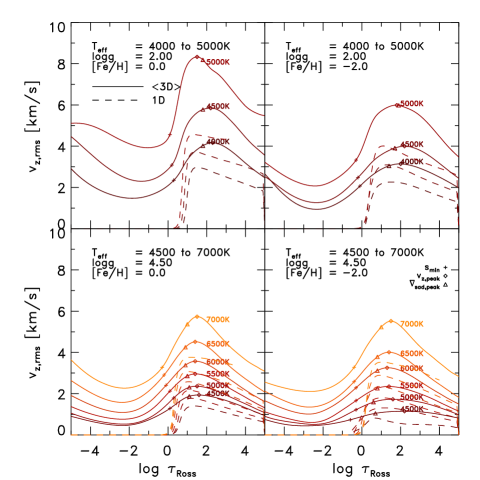
Next, we consider the velocity field in our simulations, which arise self-consistently from the solution of the hydrodynamic equations. In Fig. 17 we show the rms-velocity of the vertical component $v_{z,\mathrm{rms}}$, being the flux carrying component of the convective flows, and being the broadening component of spectral lines at disk center.

The buoyant uprising plasma will experience increasingly a decrease in density towards the photosphere, hence a strong density gradient, and due to mass conservation, the convective motions will eventually overturn. Therefore, $v_{z,\mathrm{rms}}$ peaks in the SAR around $\log\tau_{\mathrm{Ross}}\sim 1.5$ for dwarfs and $\sim 2.3$ for giants. Furthermore, since in the SAR, the transition region from convective to radiative transport of energy takes place due to decrease in opacity and the subsequent radiative losses, here we find the strongest turbulent motions concomitant with the greatest fluctuations in all thermodynamical quantities (in particular entropy, temperature and density, see Figs. 24, 13 and 18). Further towards the interior, $v_{z,\mathrm{rms}}$ drops as the density increases. From the slightly sub-photospheric maximum, velocities fall off to a minimum above the optical surface, then increases again in the higher atmosphere (see Fig. 17). Towards upper layers, $v_{z,\mathrm{rms}}$ increases again due to p-modes, excited in the SAR but leaking out of the acoustic cavity as they have frequencies above the acoustic cut-off. The metal poor simulations show a slightly smaller increase in $v_{z,\mathrm{rms}}$, since their density gradients are shallower due to steeper $T$-gradients. The declining velocity above the surface is due to the fact that the convective motions overshoot well above the top of the convection zone. We find the velocity minimum to occur between $\log\tau_{\mathrm{Ross}}\sim-2.3$ for dwarfs and $-1.5$ for giants.

As expected, the magnitude of the velocity field is enhanced towards higher $T_{\mathrm{eff}}$, lower $\log g$, and higher $\left[\mathrm{Fe}/\mathrm{H}\right]$, similar as $\Delta s$. The symmetry of the velocity profile changes with $\log g$ and metallicity, while it is little affected by $T_{\mathrm{eff}}$. For lower $\log g$, the peak in the velocity field is increasingly shifted to optically deeper layers (e.g. at solar metallicity the average peak position for dwarfs is $\left\langle\log\tau_{\mathrm{Ross}}\right\rangle\sim 1.5$, while for giants it is $\sim 2.0$). The coolest metal-poor simulations display a flatter profile, and the position of the minimum is increasingly shifted towards higher layers, especially for extreme metal-poor dwarfs ($\left[\mathrm{Fe}/\mathrm{H}\right]<-3.0$), and the profile is therefore stretched and skewed.

For comparison, we also show in Fig. 17 the convective velocity $v_{\mathrm{MLT}}$ of our 1D models determined by MLT. It is apparent that the general trends of increasing velocities with increasing $T_{\mathrm{eff}}$ and $\left[\mathrm{Fe}/\mathrm{H}\right]$ and decreasing $\log g$, are common between the simulations and the 1D MLT models, although much less pronounced in 1D. Furthermore, $v_{\mathrm{MLT}}$ drops rather sharply at the top of the convection zone (as given by the Schwarzschild criterion), as no overshooting is allowed for in our implementation of MLT. Several non-local variants of MLT exists, and they allow for overshooting, but none of them produce velocity profiles close to that of our simulations. We also want to mention the large asymmetry in velocities of the up- and downflows (SN98): in 3D simulations, the latter are much faster than the former (up to $\sim 2$ faster, in particular for cool dwarfs), contrary to what is normally assumed in 1D descriptions of convection.

Figure 18: Overview of the entropy jump (top panel), maximal vertical rms-velocity below the surface $v_{z,\mathrm{rms}}^{\mathrm{peak}}$ (middle panel) and the density at the same height $\rho_{\mathrm{peak}}$ (bottom panel) vs. $T_{\mathrm{eff}}$ for $\left[\mathrm{Fe}/\mathrm{H}\right]=-2.0$ and $0.0$ (blue and black respectively). Models with the same gravity are connected with their respective functional fits (solid lines; see App. B). Note the inverse correlation between density and velocity.

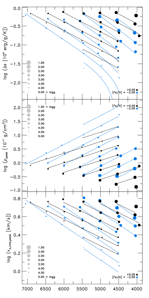
The peak vertical rms-velocity, $v_{z,\mathrm{rms}}^{\mathrm{peak}}$ (see bottom panel of Fig. 18), is a good measure of the global magnitude of velocities in the simulations. It also serves as a measure of the amount of turbulence present in the simulations. The actual values are also given in Col. 9 in Table 4, together with a functional fit in App. B. The variation of $v_{z,\mathrm{rms}}^{\mathrm{peak}}$ with stellar parameters resembles that of the entropy jump $\Delta s$ (compare top and bottom panel in Fig. 18), namely it also increases exponentially with higher $T_{\mathrm{eff}}$ and lower $\log g$ and linearly with $\left[\mathrm{Fe}/\mathrm{H}\right]$. An interesting aspect is the increase of $v_{z,\mathrm{rms}}^{\mathrm{peak}}$ and $\Delta s$ with $T_{\mathrm{eff}}$, which are close to exponential, indicating a correlation between the two. The characteristic variations of $v_{z,\mathrm{rms}}^{\mathrm{peak}}$ correspond to the inverse variations of the density taken at the same heights as the peaks in $v_{z,\mathrm{rms}}$ (see middle panel in Fig. 18). This behavior arises due to conservation of mass (Eq. 1), which can be expressed as

$$\left\langle\partial_{z}\ln\rho\right\rangle=-\left\langle\partial_{z}\ln v_{z}\right\rangle$$ (19)

for a stationary flow ($\partial_{t}\rho=0$). Of course, under this assumption, this equation is strictly speaking valid only locally, while we compare here averaged values. Despite that, we find that this relation is, in general, qualitatively fulfilled across the whole depth of our simulations. Towards the optical surface, the density decreases, which has to be compensated by faster velocities, in order to fulfill conservation of mass as well as sustain the energy flux. The velocity field profile results ultimately from the interplay between the vertical and horizontal acceleration due to buoyancy and overturning respectively. The latter in turn is set by the radiative losses that arises from the prevailing opacity conditions according to the thermodynamic state of the plasma (see Sect. 3.2.8). Furthermore, one can also reason that at a higher effective temperature, hence hotter temperature stratification, the density will be lower (ideal gas gives $T\propto 1/\rho$; see also middle panel in Fig. 18), however, at the same time, more energy (enthalpy) has to be carried to the surface, which necessitates a faster flow (as is given in Eq. 23). The entropy jump, density, and velocity are coupled intimately with each other (the vertical mass flux is $j_{z}=\rho v_{z}$). Therefore, changes in one quantity imply corresponding variations in the values of the other quantities, and vice versa. The radiative energy losses at the photospheric transition generate the entropy fluctuations according to the prevailing opacity and the irradiation-duration, hence it sets the amplitude of the entropy jump $\Delta s$. On the other hand, the entropy deficient plasma with its density excess determines the buoyancy force, $f_{B}\sim\Delta\rho$, and therefore the vertical velocities $v_{z}$ of the downdrafts. The downdrafts in turn will settle the upflows in order to deliver the required convective energy flux. The subtle details in the chain of causalities are non-trivial and beyond the scope of the present paper.

Figure 19: Comparison of the entropy jump $\Delta s$ (top panel) and the density at the optical depth of the maximal vertical velocity below the optical surface $\rho_{\mathrm{peak}}$ (bottom panel) vs. maximal vertical rms-velocity $v_{z,\mathrm{rms}}^{\mathrm{peak}}$ for all models. A linear fit is also indicated in both panels (red lines).

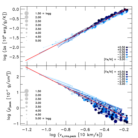
Similar to our finding in Sect. 3.1.3 of a scaling relation between the entropy jump and the constant entropy value of the adiabatic convection zone $\Delta s\left(s_{\mathrm{bot}}\right)$, we find here again another interesting, tight scaling relations between $\rho_{\mathrm{peak}}$, $v_{z,\mathrm{rms}}^{\mathrm{peak}}$ and $\Delta s$, which we show in Fig. 19. The values are plotted on a double logarithmic scale, to more clearly illustrate the power-law character of the relations. From the above discussion, it follows that the vertical velocity is also correlated with the constant entropy value $s_{\mathrm{bot}}$ of the adiabatic convection zone and the density. We also show linear fits of the density $\rho_{\mathrm{peak}}$ and entropy jump $\Delta s$ as a function of $v_{z,\mathrm{rms}}^{\mathrm{peak}}$ in log-log scale (red lines in Fig. 19), exhibiting the slopes of $\log\Delta s/\log v_{z,\mathrm{rms}}^{\mathrm{peak}}\sim 0.46$ and $\log\rho_{\mathrm{peak}}/\log v_{z,\mathrm{rms}}^{\mathrm{peak}}\sim-1.20$, hence a scaling with the respective slopes.

In 3D RHD simulations, the non-thermal, macroscopic velocity fields arising from convective instabilities are computed self-consistently from first principles and therefore have an immediate physical meaning. They represent the buoyant motions associated with convection and its turbulent features, and their statistical properties carry equally important physical information as the mean temperature or density stratifications. By contrast, in 1D atmosphere modeling, a free-parameter-dependent velocity field $v_{\mathrm{MLT}}$ is derived for the convective flux in MLT. Also, for radiative transfer and spectral line formation calculations, two ad-hoc Gaussian velocity distributions – the so-called micro- and macroturbulence ($\xi_{\mathrm{turb}}$ and $\chi_{\mathrm{turb}}$, respectively) – are usually introduced to model Doppler broadening of spectral lines associated with non-thermal (e.g., convective, turbulent, oscillatory, etc.) gas motions in stellar atmospheres. The values of the micro- and macroturbulence parameters are determined by comparing synthetic and observed spectral line profiles and line strengths. Usually, a depth-independent value of the microturbulence $\xi_{\mathrm{turb}}$ and one global value of the macroturbulence $\chi_{\mathrm{turb}}$ are applied in theoretical spectrum syntheses with 1D model atmospheres. Full-3D line formation calculations using 3D models similar to those described here, have demonstrated that in late-type stars the required non-thermal Doppler line broadening is indeed primarily the result of Doppler shifts from the convective motions and to a lesser extent oscillations in the atmosphere (Asplund et al. 2000). As such this non-thermal velocity field is clearly depth-dependent, while micro- and macroturbulence are almost always assumed to be non-varying with depth. Furthermore, $v_{\mathrm{MLT}}$ is solely assigned to satisfy the necessary amount of convective flux by the individual prescription of MLT. While, interestingly, $v_{\mathrm{MLT}}$ mimics to a certain extent the run of $v_{z,\mathrm{rms}}$ in the interior for cooler dwarfs. We remark that this interpretation is however not physically consistently motivated. Moreover, the convective velocity varies depending on its actual implementation (e.g. Böhm-Vitense 1958; Henyey et al. 1965) and, as such, $v_{\mathrm{MLT}}$ should be interpreted and used with caution. We point out that one important motivation for conducting 3D RHD atmosphere models is the fact that the before mentioned spurious inconsistent velocities become redundant. The hydrodynamical simulations account consistently for only one unique velocity field.

Figure 20: $\left\langle 3\mathrm{D}\right\rangle$ stratification of the absolute value of the vorticity $\left|\@vec{\omega}\right|$ vs. $T_{\mathrm{eff}}$ is shown for various stellar parameters.

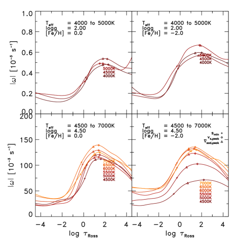
Another good measure for the turbulence of a velocity field is the absolute value of the vorticity $\left|\@vec{\omega}\right|=\left|\@vec{\nabla}\times\@vec{v}\right|$, which is shown in Fig. 20. The vorticity arises below the surface in SAR due the overturning of the upflows and the turbulent downdrafts experiencing the density gradient. The peak in $\@vec{\omega}$ is associated with pronounced shear flows, which arise due deflection of the horizontal flows into downdrafts of the overturning plasma (see SN98). The vorticity is concentrated in tube-like structures in the intergranular lanes around the edges of granules. The run of the vorticity follows closely that of $v_{z,\mathrm{rms}}$ (see Fig. 17).

3.2.3 Turbulent pressure

Figure 21: The fraction of turbulent pressure to total pressure $p_{\mathrm{turb}}/p_{\mathrm{tot}}$ vs. optical depth $\log\tau_{\mathrm{Ross}}$ is displayed for various stellar parameters.

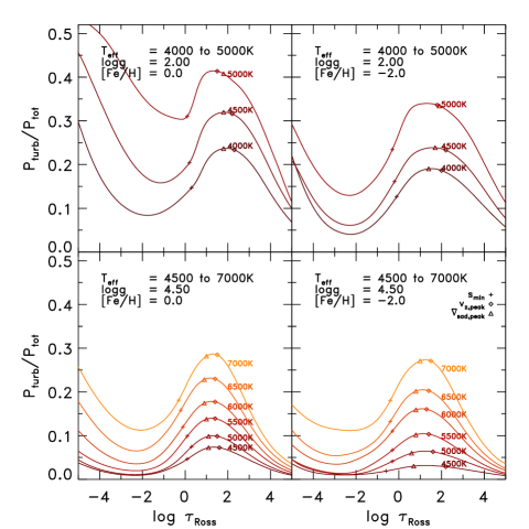
The turbulent pressure, $p_{\mathrm{turb}}=\rho v_{z}^{2}$, is an additional (dynamical) pressure that arises from the (macroscopic) vertical bulk flows due to the convective motions. It appears when considering the horizontal averages of the momentum equation (Eq. 2), more specifically of the advection term therein. The ratio of turbulent to total pressure, $p_{\mathrm{turb}}/p_{\mathrm{tot}}$, shown in Fig. 21, follows qualitatively very closely the run of $v_{z,\mathrm{rms}}$ (compare with Fig. 17), namely, it peaks in the SAR ($\log\tau_{\mathrm{Ross}}\sim 1.5$), reaches a minimum around $\log\tau_{\mathrm{Ross}}\sim-2.0$, and increases in the upper layers (a functional fit for $\left[p_{\mathrm{turb}}/p_{\mathrm{tot}}\right]_{\mathrm{peak}}$ is given in App. B). In the SAR, the shape of the $p_{\mathrm{turb}}/p_{\mathrm{tot}}$ profile with optical depth looks similar to a Gaussian function, however, towards lower $T_{\mathrm{eff}}$ and metallicity, it becomes increasingly skewed. Averages on constant geometrical depth $\left\langle\mathrm{3D}\right\rangle_{z}$ are similar, only the peak and the upper layers are slightly lower at higher $T_{\mathrm{eff}}$s.

For hotter stars, in particular metal-rich giants, the turbulent pressure becomes comparable to the gas pressure ($p_{\mathrm{turb}}/p_{\mathrm{tot}}\sim 0.4$) in the SAR, and the atmosphere is increasingly supported by $p_{\mathrm{turb}}$. This means that neglecting the turbulent pressure, as is usually done in 1D models, would significantly overestimate the gas pressure. The consequence of this is a faulty, inconsistent stratification, since the overestimation in gas pressure comes at the cost of altering other physical quantities like the density, even when the temperature stratification looks similar compared to a $\left\langle 3\mathrm{D}\right\rangle$ model.

We find that $v_{z,\mathrm{rms}}$ is very close to $v_{\mathrm{turb}}=\left[\left\langle p_{\mathrm{turb}}\right\rangle/\left\langle\rho\right\rangle\right]^{1/2}$, since the latter is basically the density-weighted analog of the former. In 1D stellar structure models that include turbulent pressure, the convective velocity from MLT is considered, i.e. $p_{\mathrm{turb,1D}}=\beta\rho v_{\mathrm{MLT}}^{2}$. However, as shown in Fig. 17, the convective velocities, $v_{\mathrm{MLT}}$, are underestimating $v_{\mathrm{turb}}$ systematically towards higher $T_{\mathrm{eff}}$ and lower $\log g$. Therefore, the 1D models can be improved by using $v_{z,\mathrm{rms}}$ resulting from 3D simulations, or one can fit the scaling factor $\beta$ to match $v_{z,\mathrm{rms}}$, which would clearly reduce the error.

As shown by Wende et al. (2009), we also expect $v_{z,\mathrm{rms}}$ to correlate with the microturbulence $\xi_{\mathrm{turb}}$, since $v_{z,\mathrm{rms}}$ is a horizontal average of the velocity field. In 1D line formation calculations, a depth-independent $\xi_{\mathrm{turb}}$ is introduced in order to compensate for missing Doppler broadening in the line extinction profile. The actual correlation of the velocity field with $\xi_{\mathrm{turb}}$ is nontrivial due to the non-locality of the radiation field, which is additionally impeded by non-linear atomic physics. Therefore, this correlation has to be determined empirically by comparing the results of 3D line-formation calculations with their $\left\langle 3\mathrm{D}\right\rangle$ counterparts (see also Steffen et al. 2009). We intend to perform such calculations in an upcoming work.

Finally, Chiavassa et al. (2011) showed that using a realistic turbulent pressure contribution to the hydrostatic equilibrium in 1D red supergiant atmospheres, greatly improves the derived surface gravity in these stars. This extra pressure component also leads to an expansion of the atmosphere compared to a 1D model stratification without turbulent pressure. This is referred to as atmospheric levitation (see Trampedach 2001). This will affect p-modes by affording them a larger cavity, and hence lowering their frequencies. This is part of the seismic near-surface effect which has plagued helio- and asteroseismology.

3.2.4 Total pressure and density

Figure 22: We display the $\left\langle 3\mathrm{D}\right\rangle$ total pressure $p_{\mathrm{tot}}$ against the optical depth $\log\tau_{\mathrm{Ross}}$ for various stellar parameters (solid lines). For comparison we also plot the 1D models with dashed lines. Note the different ordinate scale in the top panel.

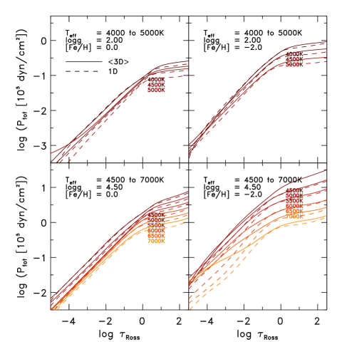
The total pressure is defined as the sum of thermodynamic and turbulent pressure, $p_{\mathrm{tot}}=p_{\mathrm{th}}+p_{\mathrm{turb}}$, and the former consists of gas and radiation pressure, $p_{\mathrm{th}}=p_{\mathrm{gas}}+p_{\mathrm{rad}}$. In Fig. 22, we show the total pressure for various stellar parameters. In contrast to the previous quantities, $p_{\mathrm{tot}}$ decreases with higher $T_{\mathrm{eff}}$, lower $\log g$, and higher metallicity. From the three stellar parameters, the influence of the metallicity is the strongest. We find the highest pressures (and densities) in the coolest metal-poor dwarfs and the lowest pressures in the hottest metal-rich giants. In the upper layers of hot metal-poor dwarfs, we find pressures systematically increased with respect to their 1D counterparts, which is accompanied by similar behavior in $\rho$, $p_{\mathrm{gas}}$ and $p_{\mathrm{turb}}$. As we showed above, a significant fraction of the total pressure is contributed by turbulent pressure in the SAR and in the upper layers (see Fig. 21), in particular towards higher $T_{\mathrm{eff}}$ and lower $\log g$. Moreover, we note that the temporal and horizontal $\left\langle\mathrm{3D}\right\rangle_{z}$-averages from our relaxed simulations are very close to hydrostatic equilibrium, and the turbulent pressure contributes significantly to this equilibrium.

Since the mean density stratifications look qualitatively similar to the total pressure ones, we refrain from showing them. Instead we prefer to show, in Fig. 18, the peak density $\rho_{\mathrm{peak}}$, which is the density at the height of the maximum rms-vertical velocity (see Fig. 17). The density $\rho_{\mathrm{peak}}$ increases with lower $T_{\mathrm{eff}}$, higher $\log g$, and lower $\left[\mathrm{Fe}/\mathrm{H}\right]$. These variations with stellar parameters arise due to the radiative transfer, since the cooling and heating rates (see Eq. 4) depend on density $\rho$ and opacity $\kappa$. We showed in Sect. 3.1.2 that with higher metallicity and opacity, the hydrostatic stratification is set at lower $\rho$.

3.2.5 Electron number density

Figure 23: We present the $\left\langle 3\mathrm{D}\right\rangle$ stratifications of the local electron number density $n_{\mathrm{el}}$ against optical depth $\log\tau_{\mathrm{Ross}}$ for various stellar parameters (solid lines). For comparison, we also show the corresponding stratifications from 1D models (dashed lines).

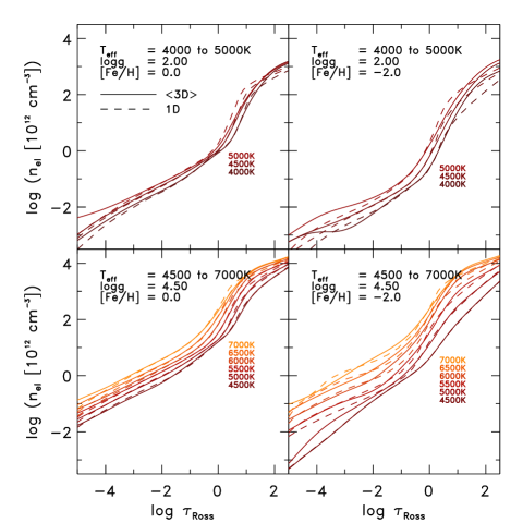
Next, we discuss the properties of the electron number density $n_{\mathrm{el}}$ (Fig. 23), which is the temporal and spatial average of the local electron density on layers of constant Rosseland optical depth. The electron number density drops by about $\sim 2\,\mathrm{dex}$ at the transition from the interior to the photosphere. This is due to the fact that the density itself decreases here, and due to the recombination of hydrogen at the photospheric transition. The convective flux consists to $\sim 1/3$ of $F_{\mathrm{ion}}$ (see Sect. 3.2.8), therefore, as the hot ionized plasma reaches the surface, it radiates away energy, recombines, and overturns into downdrafts, thereby reducing the number of free electrons. The electron density increases with higher $T_{\mathrm{eff}}$, lower $\log g$, and higher $\left[\mathrm{Fe}/\mathrm{H}\right]$. The electron pressure $p_{\mathrm{el}}=n_{\mathrm{el}}k_{\mathrm{B}}T$ follows similar trends as the electron density in terms of variations with stellar parameters and depth.

3.2.6 Entropy

Figure 24: $\left\langle 3\mathrm{D}\right\rangle$ and $\left\langle 3\mathrm{D}\right\rangle_{z}$ mean stratifications (solid and dashed respectively) of the entropy $s$ vs. the total pressure normalized to the pressure at the optical surface $\log p_{\mathrm{tot}}/p_{\mathrm{surf}}$ for various stellar parameters. We show also the $s$-stratifications of the 1D models (dotted lines). Note the different ordinate scale in the top panel.

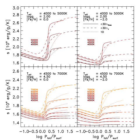
Local, box-in-a-star, 3D RHD atmosphere models have well defined boundary conditions at the bottom boundary because of the adiabaticity of the convection zone, even though they are relatively shallow and comprise only a small fraction of the convection zone. Indeed, the specific entropy per unit mass of the plasma stays constant across most of the convective zone, in particular for the upflows. In Fig. 24, we show the average entropy. Below the optical surface, the entropy converges asymptotically against $s_{\mathrm{bot}}$ into deeper layers, especially the averages on constant geometrical height $\left\langle 3\mathrm{D}\right\rangle_{z}$ (dashed lines). As the hot plasma in the granules reaches the optical surface, it becomes transparent, thereby a large fraction of the energy is radiated away. This results in a decrease in entropy, until it reaches a minimum at the top of the convection zone ($\log\tau_{\mathrm{Ross}}\sim 0.0$). Further up, the entropy then increases again due to the decoupling of the radiation and matter above the photosphere, which results in an almost isothermal atmosphere. The 1D models (dotted lines) exhibit larger entropy stratifications in the deeper convection zone, in particular for higher $T_{\mathrm{eff}}$, thereby overestimating the entropy jump increasingly due to the fixed mixing-length parameter $\alpha_{\mathrm{MLT}}$ with 1.5 for all stellar parameters.

3.2.7 Superadiabatic temperature gradient

Figure 25: We show the $\left\langle\mathrm{3D}\right\rangle_{\mathrm{Ross}}$ (solid lines) and $\left\langle\mathrm{3D}\right\rangle_{z}$ (dashed lines) superadiabatic gradient $\nabla_{\mathrm{sad}}$ vs. optical depth $\log\tau_{\mathrm{Ross}}$ for various stellar parameters. Furthermore, for comparison, we also show the corresponding values from 1D models (dotted lines). Note the different ordinate scale in the top panels.

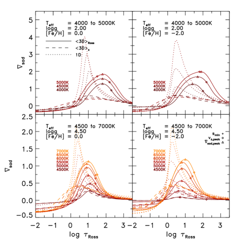
We limit ourselves to show only the superadiabatic gradient $\nabla_{\mathrm{sad}}=\nabla-\nabla_{\mathrm{ad}}$, since it combines the important properties of both the total and the adiabatic temperature gradient ($\nabla$ and $\nabla_{\mathrm{ad}}$ respectively). In Fig. 25, we show $\nabla_{\mathrm{sad}}$ averaged over constant geometrical height or Rosseland optical depth. The peak in $\nabla_{\mathrm{sad}}$, which looks like a skewed Gaussian function, arises solely from the temperature gradient $\nabla$. The superadiabatic gradient peaks around $\log\tau_{\mathrm{Ross}}\sim 1.0-2.0$, and becomes sub-adiabatic, i.e. $\nabla_{\mathrm{sad}}<0.0$, above the optical surface at $\log\tau_{\mathrm{Ross}}<0.0-0.5$. The entropy jump correlates directly with the superadiabatic gradient, since $\nabla_{\mathrm{sad}}=1/c_{p}\left[\partial s/\partial\ln p_{\mathrm{tot}}\right]$ and one can show that $\partial s/dz=c_{P}/H_{P}\left(\nabla-\nabla_{\mathrm{ad}}\right)$. Hence, it is no surprise that they exhibit similarity in the peak amplitude and position. In particular, the peak amplitude increases with increasing $T_{\mathrm{eff}}$ and $\log g$ (see $\Delta s$ in Fig. 18; a functional fit for $\nabla_{\mathrm{sad}}^{\mathrm{peak}}$ is given in App. B). The position of $\nabla_{\mathrm{sad}}^{\mathrm{peak}}$ on the optical depth scale $\left\langle\mathrm{3D}\right\rangle_{\mathrm{Ross}}$ (triangles), hence the position of the steepest temperature gradient, changes slightly with stellar parameters. However, similar to the position of $v_{z,\mathrm{rms}}^{\mathrm{peak}}$, in the $\varepsilon-\rho$-plane, the distribution of $\nabla_{\mathrm{sad}}^{\mathrm{peak}}$ is regular (see Fig. 16), namely it shifts systematically towards higher $\varepsilon$ and lower $\rho$ with increasing $T_{\mathrm{eff}}$.

As it is clear in Fig. 25, one finds substantial differences in $\nabla_{\mathrm{sad}}$ when comparing the two $\left\langle 3\mathrm{D}\right\rangle$ stratifications with their 1D counterparts, namely, the 1D gradients exhibit distinctively larger amplitudes. These differences arise partly due the missing turbulent pressure in the 1D case, but do not resolve the discrepancies. Furthermore, we find an asymmetrically skewed shape towards the optical surface in the 1D gradients, which is shared by the geometrical averages $\left\langle\mathrm{3D}\right\rangle_{z}$, but is not the case for the averages on constant Rosseland optical depth $\left\langle\mathrm{3D}\right\rangle_{\mathrm{Ross}}$. A main reason for the shown differences between $\left\langle\mathrm{3D}\right\rangle_{\mathrm{Ross}}$ and 1D comes from the averaging over layers of constant $\tau_{\mathrm{Ross}}$. The underlying $\nabla_{\mathrm{ad}}$s are rather insensitive to the deviations between the $\left\langle\mathrm{3D}\right\rangle_{\mathrm{Ross}}$ and 1D stratifications, so the differences arise mainly due to $\nabla$. Between $\left\langle\mathrm{3D}\right\rangle_{z}$ and 1D the adiabatic gradients differ in the sub-photospheric gradient.

3.2.8 Transport of energy

Figure 26: Behavior of the normalized energy fluxes $F/F_{\mathrm{tot}}$ against the total pressure normalized to the pressure at the optical surface $\log p_{\mathrm{tot}}/p_{\mathrm{surf}}$ as a function of variations in the individual stellar parameters ($T_{\mathrm{eff}}$, $\log g$, and $\left[\mathrm{Fe}/\mathrm{H}\right]$, from top to bottom, respectively ). In each panel, the various curves are shown varying one of the parameters while keeping the other two fixed. The individual normalized components of $F_{\mathrm{tot}}$ are $F_{\mathrm{enth}}$ (dashed), $F_{\mathrm{kin}}$ (dotted), $F_{\mathrm{ion}}$ (dash-triple-dotted), $F_{\mathrm{th}}$ (long dashed) and $F_{\mathrm{rad}}$ (solid). Averages are evaluated at constant geometrical height.

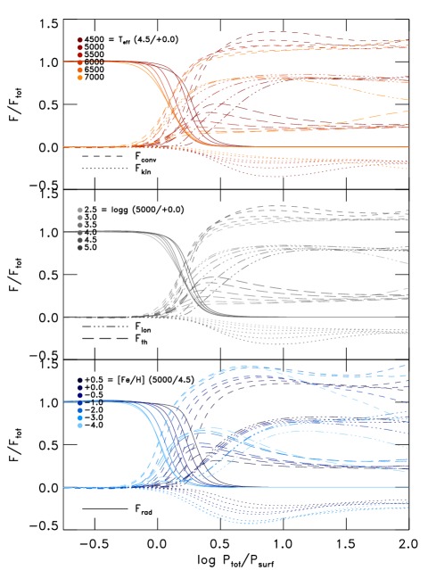
The individual energy fluxes are quantities worthy of further consideration. The energy flux is conserved only on averages of constant geometrical height $\left\langle\mathrm{3D}\right\rangle_{z}$, therefore, we show and discuss the latter here. The total energy flux $F_{\mathrm{tot}}=F_{\mathrm{rad}}+F_{\mathrm{conv}}+F_{\mathrm{visc}}$ emerges from the photosphere solely in the form of radiative energy flux. The total energy flux is supplied from the convection zone by the convective energy flux, which is the sum of the enthalpy flux

$$F_{\mathrm{enth}}=\left[\varepsilon+\frac{p_{\mathrm{th}}}{\rho}\right]\delta j_{z},\qquad\mathrm{with}\,\delta j_{z}=\rho v_{z}-\left\langle\rho v_{z}\right\rangle$$ (20)

($\delta j_{z}$ being the horizontal fluctuations of the vertical mass flux; the average vertical mass flux vanishes) carried in the upflows and the kinetic energy flux

$$F_{\mathrm{kin}}=\left[\frac{1}{2}\rho\@vec{v}^{2}\right]\delta j_{z}$$ (21)

arising from the downdrafts (see SN98 and Nordlund et al. 2009). Since the mean kinetic energy flux $F_{\mathrm{kin}}$ is negative, the positive enthalpy flux $F_{\mathrm{enth}}$ is the major component of the convective energy flux $F_{\mathrm{conv}}$. The enthalpy flux in turn consists of the energy fluxes due to ionization $F_{\mathrm{ion}}=\left[\varepsilon-\frac{3}{2}\frac{p_{\mathrm{th}}}{\rho}\right]\delta j_{z}$, thermal heat $F_{\mathrm{th}}=\frac{3}{2}\frac{p_{\mathrm{th}}}{\rho}\delta j_{z}$ and acoustic (sound) waves $F_{\mathrm{acous}}=\left\langle p_{\mathrm{th}}v_{z}\right\rangle-\left\langle p_{\mathrm{th}}\right\rangle\left\langle v_{z}\right\rangle$. In Fig. 26, we show the energy fluxes $F_{\mathrm{rad}}$, $F_{\mathrm{enth}}$, $F_{\mathrm{kin}}$, $F_{\mathrm{ion}}$, and $F_{\mathrm{th}}$ normalized to the total emergent energy flux $\sigma T_{\mathrm{eff}}^{4}$ (for clarity, we refrain from showing $F_{\mathrm{visc}}$ and $F_{\mathrm{acous}}$, since their contribution to $F_{\mathrm{tot}}$ is very small). We vary one stellar parameter at a time, while the other two are fixed ($T_{\mathrm{eff}}$, $\log g$, and $\left[\mathrm{Fe}/\mathrm{H}\right]$, from top to bottom in Fig. 26, respectively). Just below the optical surface ($0.5<\log p_{\mathrm{tot}}/p_{\mathrm{surf}}<1.0$), both $F_{\mathrm{kin}}$ (solid lines) and $F_{\mathrm{enth}}$ (dashed lines) increase towards cool metal-poor dwarfs, i.e. lower $T_{\mathrm{eff}}$, $\left[\mathrm{Fe}/\mathrm{H}\right]$ and higher $\log g$, due to higher densities and velocities. The increased reduction of the total flux by $F_{\mathrm{kin}}$ ($<0.0$) is compensated by a simultaneously higher $F_{\mathrm{enth}}$ ($>1.0$). On the other hand, in deeper layers ($\log p_{\mathrm{tot}}/p_{\mathrm{surf}}>1.5)$, both converge to similar fractions for all stellar parameters ($-0.17$ and $1.14$ for $F_{\mathrm{kin}}$ and $F_{\mathrm{enth}}$ respectively). This convergence to very similar values is rather remarkable. The convective motions seem to follow an exact guideline, which might be correlated to the universal filling factor, however, we will study this more carefully in a future work. We remark that in deeper solar simulations ($20\,\mathrm{Mm}$) that $F_{\mathrm{enth}}$ and $F_{\mathrm{kin}}$ increase with depth, while their sum remains constant (see Stein et al. 2009).

The majority of the total energy flux $F_{\mathrm{tot}}$ in the convection zone is carried in form of ionized hydrogen with $F_{\mathrm{ion}}\simeq 0.67$, while thermal heat is the second most important component with $F_{\mathrm{th}}\simeq 0.29$. The acoustic energy constitutes only a small fraction with $F_{\mathrm{acous}}\simeq 0.04$. SN98 found similar fractions with $F_{\mathrm{kin}}\sim-0.10$ to $-0.15$, $F_{\mathrm{ion}}\sim 2/3$ and $F_{\mathrm{th}}\sim 1/3$ for the Sun. The $F_{\mathrm{ion}}$ and $F_{\mathrm{th}}$ fractions, which are the major constituents of the enthalpy flux, undergo a significant change below the surface, as we show in Fig. 26 for models with different stellar parameters. In particular, the fraction of thermal heat $F_{\mathrm{th}}$ becomes more significant at the cost of $F_{\mathrm{ion}}$ towards cool metal-poor dwarfs. The thermal flux $F_{\mathrm{th}}$ reaches a maximum (up to $F_{\mathrm{th,max}}\simeq 0.5$) just below the surface, but eventually converges close to the above mentioned fractions in deeper layers (long dashed lines).

In 1D MLT models, the convective flux is assumed to consist of the enthalpy flux only, $F_{\mathrm{conv,1D}}$ (see Appendix A.1). This is a result of the MLT assumption of symmetric flows which means that the kinetic energy fluxes in the up- and downflows cancel exactly. As remarked by Henyey et al. (1965), the details on $F_{\mathrm{kin}}$, $F_{\mathrm{ion}}$, $F_{\mathrm{th}}$ and $F_{\mathrm{acous}}$ are not at hand due to the lack of a self-consistent velocity field. The energy fluxes from 3D RHD simulations, on the other hand, arise self-consistently from solving the coupled equations of radiative hydrodynamics, without further assumptions.

As mentioned above, the emergent total energy flux $F_{\mathrm{tot}}$ is carried in the convection zone mainly by the positive enthalpy flux $F_{\mathrm{enth}}$ (Eq. 20). Therefore, one can approximate the convective energy flux with the mean jump in enthalpy $\Delta h$ times the mean vertical mass flux of the upflows below the optical surface, hence

$$F_{\mathrm{conv}}\approx\left\langle\Delta h\right\rangle\left\langle\rho v_{z}\right\rangle.$$ (22)

At the transition region, the enthalpy jump $\Delta h$ is primarily caused by the strong drop in internal energy $\varepsilon$, hence entropy $s$, and the thermodynamic pressure work is rather small (note the change of $p_{\mathrm{tot}}$ below the surface $\log\tau_{\mathrm{Ross}}>0.0$ in Fig. 22), i.e. $\Delta h\approx T\Delta s$, where $T$ is the temperature at the surface. By approximating $T\simeq T_{\mathrm{eff}}$, one can expect the total energy flux $F_{\mathrm{tot}}=\sigma T_{\mathrm{eff}}^{4}$ to depend to first order on the mean entropy jump, density, and vertical velocity:

$$\sigma T_{\mathrm{eff}}^{3}\propto\left\langle\Delta s\right\rangle\left\langle\rho\right\rangle\left\langle v_{z}\right\rangle.$$ (23)

This approximation can already be retrieved on dimensional grounds, however, we derived the latter in order to explain the systematic variations of $\Delta s$, $v_{z,\mathrm{rms}}^{\mathrm{peak}}$ and $\rho_{\mathrm{peak}}$ with stellar parameters, which we have observed above (see Figs. 5, 18 and 18, respectively). The emergent radiative energy flux is correlated with $\Delta s$, $\rho$ and $v_{z}$, and the respective composition resulting from the individual contributions varies with stellar parameters.

The interplay between the radiative heating and cooling rates $q_{\mathrm{rad}}$ (Eq. 4) and hydrostatic equilibrium, require a different density stratification for different stellar parameters due to the dependence of opacity on thermodynamic variables, as we showed in Sect. 3.1.2. The resulting density variations will induce adjustments in the vertical velocity and entropy jump. Furthermore, we find with increasing $\log g$ and $\left[\mathrm{Fe}/\mathrm{H}\right]$ at a fixed $T_{\mathrm{eff}}$, the density increases, which is compensated by higher $\Delta s$ and $v_{z}$ ($\Delta s\propto\Delta\rho^{-1}$, see Eq. 15). We would like also to emphasize the remarkably important (non-local) influence of the rather thin photospheric transition region on basically the whole convection zone, since the entropy deficiency of the turbulent downdrafts are generated mainly here. The latter sets the entropy jump and the convective driving (see Nordlund et al. 2009).

Figure 27: We show the normalized cooling and heating rates $q_{\mathrm{rad}}^{\mathrm{norm}}$ vs. optical depth $\log\tau_{\mathrm{Ross}}$ for various stellar parameters. The shown averages are retrieved on constant geometrical height $\left\langle 3\mathrm{D}\right\rangle_{z}$. Note the different ordinate scale in the top panel.

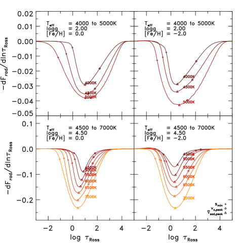
The radiative heating and cooling rates $q_{\mathrm{rad}}$ (Eq. 4) due to radiative losses enter the hydrodynamic equations as a source and sink term in the energy equation (Eq. 3). It is the divergence of the radiative flux $q_{\mathrm{rad}}=-\@vec{\nabla}\cdot\@vec{F}_{\mathrm{rad}}$, and a large, negative $q_{\mathrm{rad}}$, the cooling peak, marks the transition of energy transport from fully convective below the optical surface to fully radiative close to the photosphere. To better illustrate the depth dependence of $q_{\mathrm{rad}}$ and the comparison among different models, in Fig. 27, we show the normalized cooling and heating rates $q_{\mathrm{rad}}^{\mathrm{norm}}=-dF_{\mathrm{rad}}/d\ln\tau_{\mathrm{Ross}}$. One can see that the amplitude of $q_{\mathrm{rad}}^{\mathrm{norm}}$ increases with higher $T_{\mathrm{eff}}$, accompanied by an increase in the width of the cooling peak. The position of the maximum absolute amplitude coincides with the position of $\nabla_{\mathrm{sad}}^{\mathrm{peak}}$, since the cooling rate (radiative loss) is setting the entropy fluctuations, hence the superadiabatic gradient (see Sect. 3.2.7). Furthermore, this location moves into upper layers for higher $T_{\mathrm{eff}}$ (from $\log\tau_{\mathrm{Ross}}\simeq 1.0$ up to $0.2$ for $T_{\mathrm{eff}}=4000$ to $7000\,\mathrm{K}$ respectively). On the other hand, the width of the photospheric transition region $\Delta_{\mathrm{ph}}=\Delta\log\tau_{\mathrm{Ross}}\left(q_{\mathrm{rad}}<0\right)$ clearly widens for hotter $T_{\mathrm{eff}}$, but also, in particular, for metal-poor giants (see top right panel in Fig. 27). While for cool dwarfs the width is typically $\Delta_{\mathrm{ph}}\approx 3.0\,\mathrm{dex}$, for hot metal-poor giants, it reaches $\Delta_{\mathrm{ph}}\approx 5.0\,\mathrm{dex}$ (see, e.g., model with $5000\,\mathrm{K}$ in right top panel of Fig. 27).

3.3 Comparison with 1D models

3.3.1 1D models

Figure 28: Comparison of the temperature stratification for the $\left\langle 3\mathrm{D}\right\rangle$ and the 1D models by showing the difference $\left\langle 1\mathrm{D}\right\rangle-\left\langle 3\mathrm{D}\right\rangle$ (colored bars) between $\log\tau_{\mathrm{Ross}}=-5.0$ and $2.0$ in the Kiel-diagram. We present four different metallicity ($\left[\mathrm{Fe}/\mathrm{H}\right]=-3.0,-2.0,-1.0$ and $0.0$).

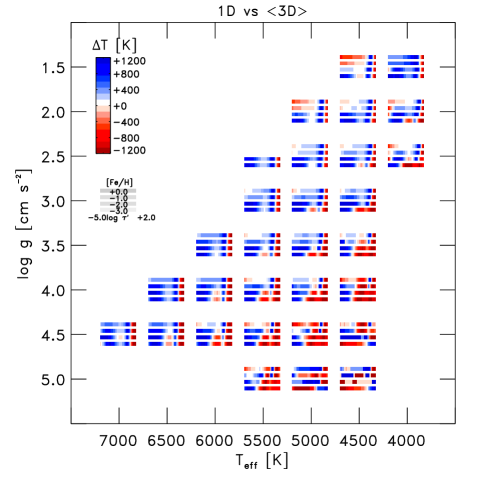
A differential comparison between 1D and 3D in terms of approaches in the modeling of stellar atmospheres is of obvious relevance here. Therefore, we developed a plane-parallel, hydrostatic, 1D atmosphere code (hereafter simply referred to as the 1D code) that is based on a similar physical treatment as the MARCS code with a few simplifications (see Appendix A and Gustafsson et al. 2008 for more details). We employ exactly the same EOS and opacities as in the individual 3D models, thereby excluding differences due to dissimilar input physics. Also, we applied the $\left\langle\mathrm{3D}\right\rangle$ models as initial stratifications for the 1D models. These mean $\left\langle\mathrm{3D}\right\rangle$ stratifications are defined on an equidistant optical depth scale from $\log\tau_{\mathrm{Ross}}=-5.0$ to $+5.0$ in steps of $0.1$. The well-resolved optical depth scale reduces discretization errors in the 1D atmosphere calculations, thereby making the 1D-$\left\langle\mathrm{3D}\right\rangle$ comparison more reliable.

In Fig. 28, we show a comparison of the 1D and $\left\langle 3\mathrm{D}\right\rangle$ temperature stratifications. One can immediately extract that the upper layers of the atmospheres are systematically overestimated in the 1D models by up to $\sim 1000\,\mathrm{K}$, in particular for metal-poor stars $\left[\mathrm{Fe}/\mathrm{H}\right]\leq-2.0$ (for solar models the maximal difference is $\sim 500\,\mathrm{K}$). In the optically thin layers of 1D models, stable against convection, radiative equilibrium is enforced. However, in the upper layers of the metal-poor $\left\langle\mathrm{3D}\right\rangle$ models, the effect of the non-vanishing adiabatic cooling rate is to shift the balance with radiative heating to lower temperatures due to a scarcity and weakness of spectral lines at lower metallicities (Asplund et al. 1999a; Collet et al. 2007). Interesting are also the hotter temperature stratifications for a few giants ($T_{\mathrm{eff}}/\log g=4500\,\mathrm{K}/1.5$ and $5000\,\mathrm{K}/2.0$) towards higher metallicity ($\left[\mathrm{Fe}/\mathrm{H}\right]>-2.0$), which results from the radiative equilibrium at higher temperatures. On the other hand, with the 1D models, we find systematically cooler temperatures below the photosphere $\log\tau_{\mathrm{Ross}}\simeq 2.0$ with up to $\sim 1000\,\mathrm{K}$ (here there is no difference with different metallicities). Therefore, one has to keep in mind that, with 1D atmosphere models, and for metal-poor stars in particular, these severe effects on the stratifications can lead to large systematic errors in spectroscopic abundance determinations, up to 0.5 dex or more in logarithmic abundance, depending on the formation height of the individual spectral lines used in the analysis (e.g. Asplund et al. 1999a; Asplund & García Pérez 2001; Collet et al. 2006, 2007; Caffau et al. 2008, 2011; González Hernández et al. 2010; Kučinskas et al. 2013). We will return to this issue using our new grid of 3D stellar models in subsequent investigations.

In the 1D model calculations the mixing-length parameter is kept constant with $\alpha_{\mathrm{MLT}}=1.5$, which is the commonly applied value (see Gustafsson et al. 2008). However, it is well-known that $\alpha_{\mathrm{MLT}}$ varies with stellar parameters (see Ludwig et al. 1999; Bonaca et al. 2012, Magic et al. in preparation). Therefore, we caution that a single fixed value will lead to severe differences in atmospheric stratification. The systematic deviations beneath the optical surface in the temperature stratification between 1D and $\left\langle\mathrm{3D}\right\rangle$ towards cool dwarfs can be interpreted as the manifestation of the wrong $\alpha_{\mathrm{MLT}}$ (see Fig. 28). Furthermore, $p_{\mathrm{turb}}$ is neglected in the 1D code, which affects the stratification by reducing the gas pressure (see Sect. 3.2.3).

3.3.2 MARCS and ATLAS models

Figure 29: Similar as Fig. 28, however here we compare the $\left\langle 3\mathrm{D}\right\rangle$ with the MARCS models for $\left[\mathrm{Fe}/\mathrm{H}\right]=-3.0,-2.0,-1.0$ and $0.0$. For a better comparison, we applied the same temperature range as given Fig. 28.

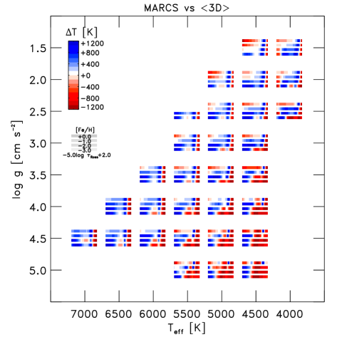
Last, we would also like to briefly compare our $\left\langle 3\mathrm{D}\right\rangle$ stratifications with the currently widely applied MARCS and ATLAS models (see Fig. 29, we show only the comparison with MARCS modes, since the ATLAS models look qualitatively rather similar). We find qualitatively similar deviations as with the 1D models above. At the same time, here we also have additional differences due to the different input physics (EOS and opacities). The largest differences between the $\left\langle 3\mathrm{D}\right\rangle$ and 1D MARCS stratifications of metal-poor stellar atmospheres are slightly higher, with $\sim 1300\,\mathrm{K}$ at $\left[\mathrm{Fe}/\mathrm{H}\right]=-3.0$, while for solar metallicity the temperatures are underestimated in 1D by $\sim 500\,\mathrm{K}$ at mosts. Below the surface, the differences amount to $\sim 1000\,\mathrm{K}$. The ATLAS models are up to $\sim 850\,\mathrm{K}$ hotter at the top and $\sim 1000\,\mathrm{K}$ cooler below the surface. In both cases, the deviations at the top increase towards lower $\left[\mathrm{Fe}/\mathrm{H}\right]$.

4 Conclusions

We presented here a comprehensive grid of realistic, state-of-the-art, three-dimensional (3D), time-dependent, radiative-hydrodynamic (RHD) stellar atmosphere models for late-type stars, covering a substantial portion of stellar parameter space, and provided a detailed description of the approach we followed for the construction of models. With the aid of our realistic 3D RHD simulations, we are able to access and render details of stellar atmospheres and subsurface convection, that are out of reach for 1D models and also inaccessible by observations. We presented and discussed a number of important global physical properties of the simulations as well as the mean stratifications resulting from the relatively large amount of data.

The constant entropy value of the adiabatic convection zone has a profound influence on several aspects and properties of the 3D RHD simulations. In particular, we find systematic correlations among the constant entropy value of the adiabatic convection zone, the entropy jump, and the vertical velocity, which we interpreted as scaling relations. In addition, we find that the variation in intensity contrast is enhanced at lower metallicity. Also, we determined that the granule size scales basically with the pressure scale height close to the surface, which can be explained in the picture of what we refer to as Nordlund scaling relation (NSR).

We discussed in great detail the depth-dependent temporal and spatial averages of various important physical quantities. In particular, we determined and examined various systematic trends in the variations of the entropy jump, the density, and the vertical velocity with stellar parameters. The latter can be discussed by regarding the changes in the transition of energy transport from convective to radiative at the photosphere. Namely, for different stellar parameters, the coupling between radiation and matter through the radiative transfer necessitates specific physical conditions due to changes in the opacity, which in turn alters the density. These variations in the density on the other hand require adjustments in the entropy jump and the vertical velocity. This can be illustrated under consideration of the total energy flux and conservation of energy. The named important values are coupled with each other, and these also set basically the general physical framework of the stellar atmosphere. The actual particular connections of these correlations have to be studied carefully in more detail, thus possibly leading to an improved understanding of the physical mechanisms operating in subsurface convection, hence stellar atmospheres.

We compared our 3D models and their mean stratifications to 1D models employing the same input physics, thereby revealing important systematic differences between the two kinds of models due to the incomplete treatment of convection by the 1D mixing-length theory (MLT) and the assumption of radiative equilibrium. The latter leads to an overestimation of the temperature stratification in metal-poor stars. While below the optical surface, we find that the temperatures are typically underestimated due to a fixed mixing length ($\alpha_{\mathrm{MLT}}=1.5$), in particular for higher $T_{\mathrm{eff}}$ and lower $\log g$. Also, we find that MLT fails to render a realistic vertical velocity field. The often neglected turbulent pressure has towards giants a non-negligible contribution on the total pressure, thereby, indicating that the thermal gas pressure is also overestimated significantly. We also quantified the differences with widely used 1D atmosphere models, in particular ATLAS and MARCS. For a number of important values we provide functional fits with stellar parameters, so that these can be accessed immediately. Thereby, one can easily scale new 3D models based on these informations.

The present work is meant to be an introduction to a series of papers on the Stagger-grid. The material discussed here is in fact just a small fraction of the actual information contained in the complete simulation data set. On the other hand, the list of potential applications for 3D models is also long. Because of space constraints, we will discuss in more detail the different methods we have applied for computing temporal and spatial averages of our 3D RHD models in a separate paper. Therein, we will also discuss our routines for the interpolation of $\left\langle 3\mathrm{D}\right\rangle$ atmosphere models, and explore the differences between $\left\langle 3\mathrm{D}\right\rangle$ and 3D line formation. We have also compiled details on statistical properties, which we will present individually. These can be later on utilized for a so-called $1.5\mathrm{D}$ line formation (see Ayres et al. 2006). An obvious plan on the agenda is also to analyze carefully the detailed properties of granulation and the intergranular lane for different stellar parameters across the HR-diagram in the future.

As the major purpose of theoretical atmosphere models, we are computing full 3D synthetic spectra with OPTIM3D (see Chiavassa et al. 2009) for all of our models (Chiavassa et al. in preparation). These will be made publicly accessible and can be used for various applications, e.g. spectroscopic parameter determination. Furthermore, we will derive new limb-darkening coefficients based on the full 3D synthetic spectra (Magic et al. in preparation), which are vital for applications such as the characterization of transiting exoplanets (Hayek et al. 2012). We intend to calibrate photometric colors and radial velocities from the spectra. For abundance determinations, we will construct an extensive library of synthetic high-resolution spectral lines. These will serve for deriving 3D effects on line-shifts, line-asymmetries and bisectors.

Also an important application is the calibration of free parameters in 1D models by employing our 3D simulations, in particular MLT and micro- and macroturbulence. We will incorporate our $\left\langle 3\mathrm{D}\right\rangle$ models into stellar evolutionary models, which will result in improved stellar structures useful for asteroseismology. And with 3D line formation calculations we will calibrate the microturbulence.

Despite the enormous success and the ab-initio nature of 3D atmosphere modeling, as last we want to mention the weaknesses. In order to keep the computation costs reasonable, the radiative transfer is simplified with the opacity binning method, which may influence the outcome. Also, the numerical resolutions of these so called large-eddy simulations are not resolving the microscopic viscous dissipation length scales, hence, the need to introduce numerical diffusion. However, these do not affect the main properties of the macroscopic flows and of the physical stratification. Also, we minimized the diffusion coefficients once under the constraint of numerical stability, and then applied for all the simulations. These issues can be solved, and the easiest rectification will be enhancement of the numerical resolution, in particular for giant. Furthermore, we will conduct improvements in the radiative transfer by employing more bins and possibly more more angles in the future. By inserting magnetic fields with different field strength, we will explore the influence of the latter on convection for different type stars. Accounting for non-LTE effects is extremely expensive for 3D simulations, therefore, these are usually neglected, however, even these will be included eventually in the future.

Appendix A The Stagger-grid 1D atmospheres

The following discussion concerns solely 1D atmosphere models and MLT, therefore, similar quantities as discussed above may deviate (e.g. $F_{\mathrm{conv}}$). The numerical code that we used for computing 1D atmospheres for the Stagger-grid models solves the coupled equations of hydrostatic equilibrium and energy flux conservation in 1D plane-parallel geometry. The 1D models use the same EOS and opacity package in order to allow consistent 3D-1D comparisons. The set of equations and numerical methods employed for their solution are similar to those of the MARCS code (Gustafsson et al. 2008) with a few changes and simplifications that will be outlined in the following. The resulting model atmospheres yet maintain very good agreement with MARCS models (see Sect. 3.3.2).

A.1 Basic equations

Assuming 1D plane-parallel geometry with horizontal homogeneity and dominance of hydrostatic equilibrium over all vertical flow simplifies the equation of motion (Eq. 2) to the hydrostatic equilibrium equation

$$\frac{d}{d\tau_{\mathrm{std}}}\left(p_{\mathrm{gas}}+p_{\mathrm{turb}}\right)-\frac{\rho g}{\kappa_{\mathrm{std}}}=0,$$ (24)

where $\kappa_{\mathrm{std}}$ and $\tau_{\mathrm{std}}$ are a standard opacity and corresponding optical depth (e.g. the Rosseland mean), $p_{\mathrm{gas}}$ and $p_{\mathrm{turb}}$ denote gas pressure and turbulent pressure, $\rho$ is the gas density, and $g$ is the surface gravity. Radiation pressure is neglected, as in the 3D simulations. Turbulent pressure is estimated using the expression

$$p_{\mathrm{turb}}=\beta\rho v_{\mathrm{turb}}^{2},$$ (25)

with the scaling parameter $\beta$ that corrects for asymmetries in the velocity distribution and the mean turbulent velocity $v_{\mathrm{turb}}$ that is used as a free, independent parameter.

The depth-integral of the energy equation (Eq. 3) reduces to the flux conservation equation,

$$F_{\mathrm{rad}}+F_{\mathrm{conv}}-\sigma T_{\mathrm{eff}}^{4}=0,$$ (26)

where $F_{\mathrm{rad}}$ is the radiative energy flux, $F_{\mathrm{conv}}$ is the convective energy flux, $\sigma$ is the Stefan-Boltzmann constant and $T_{\mathrm{eff}}$ is the stellar effective temperature. Contrary to the 3D case, effective temperature now appears as a boundary value and is thus a free parameter. Owing to numerical instabilities of the formulation, Eq. 26 is replaced in the higher atmosphere ($\tau_{\mathrm{Ross}}\lesssim 10^{-2}$) with the radiative equilibrium condition

$$q_{\mathrm{rad}}=4\pi\rho\int_{\lambda}\kappa_{\lambda}(J_{\lambda}-S_{\lambda})d\lambda\equiv 0,$$ (27)

where $J_{\lambda}$ and $S_{\lambda}$ are the mean intensity and the source function, similar to Eq. (6). In the 3D case, $q_{\mathrm{rad}}$ is explicitly calculated and is nonzero in general. Enforcing the condition of radiative equilibrium $q_{\mathrm{rad}}\equiv 0$ in 1D leads to an atmospheric stratification where an exact balance of radiative heating and cooling in each layer is achieved, ignoring the effects of gas motion.

The mean intensity and the radiative energy flux at each depth are obtained by solving the radiative transfer equation,

$$\mu\frac{dI_{\lambda}}{d\tau_{\lambda}}=I_{\lambda}-S_{\lambda},$$ (28)

where $\mu=\cos\theta$ with the polar angle $\theta$ off the vertical, $I_{\lambda}$ is the specific intensity at wavelength $\lambda$, and $\tau_{\lambda}$ is the vertical monochromatic optical depth (with $\tau_{\lambda}=0$ above the top of the atmosphere). A Planck source function $S_{\lambda}=B_{\lambda}$ is assumed. The monochromatic mean intensity and radiative flux are then delivered by the integrals

$$J_{\lambda} = \frac{1}{2}\int_{-1}^{1}I_{\lambda}d\mu$$ (29)

$$F_{\mathrm{rad},\lambda} = 2\pi\int_{-1}^{1}I_{\lambda}\mu d\mu.$$ (30)

In the absence of an explicit convection treatment, convective energy transfer is estimated using a variant of the mixing length recipe described in Henyey et al. (1965). The convective flux is given by the expression

$$F_{\mathrm{conv}}=\frac{1}{2}\alpha_{\mathrm{MLT}}\delta\Delta c_{p}T\rho v_{\mathrm{MLT}},$$ (31)

where $\rho$ is the gas density, $c_{p}$ is the specific heat capacity, $T$ is the temperature, and $v_{\mathrm{MLT}}$ is the convective velocity. The well-known free mixing length parameter $\alpha_{\mathrm{MLT}}=l_{m}/H_{p}$ sets the distance $l_{m}$ in units of the local pressure scale height $H_{p}$ over which energy is transported convectively. See Gustafsson et al. (2008) for details of the expressions used to obtain the convective velocity $v_{\mathrm{MLT}}$ and the factor $\delta\Delta=\Gamma/\left(1+\Gamma\right)\nabla_{\mathrm{sad}}$, which scales super-adiabaticity $\nabla_{\mathrm{sad}}=\nabla-\nabla_{\mathrm{ad}}$ of the atmospheric stratification (see also Sect. 3.2.7), by a convective efficiency factor $\Gamma=c_{P}\rho v_{\mathrm{MLT}}\tau_{e}(y+\tau_{e}^{-2})/(8\sigma T^{3})$ with the optical thickness $\tau_{e}=\kappa_{\mathrm{Ross}}l_{m}$. We adopt the same parameters $y=0.076$ and $\nu=8$ as Gustafsson et al. (2008) for the radiative heat loss term and turbulent viscosity that enter the above quantities.

A.2 Numerical methods

The system of equations is solved using a modified Newton-Raphson method with an initial stratification of temperature $T$ and gas pressure $p_{\mathrm{gas}}$ on a fixed Rosseland optical depth grid. Discretized and linearized versions of the hydrostatic equation and the energy flux equation (or radiative equilibrium condition, respectively) provide the inhomogeneous term and the elements of the Jacobian matrix for the system of $2N$ linear equations, where $N$ is the number of depth layers. The radiation field is computed for each Newton-Raphson iteration using the integral method, based on a second-order discretization of the fundamental solution of the radiative transfer equation (Eq. 28).

The corrections $\Delta T$ and $\Delta p_{\mathrm{gas}}$ derived from the system of linear equations are multiplied by a variable factor $<1$ that is automatically regulated by the code to aid convergence. Convergence is assumed when the (relative) residuals of the $2N$ equations decrease beneath a preset threshold. Note that, contrary to the 3D simulations, the effective temperature is now an adjustable parameter; the requirement of minimal residuals automatically leads to an atmospheric stratification with correct $T_{\mathrm{eff}}$ through the energy flux equation.

In order to obtain a 1D model, a given $\left\langle 3\mathrm{D}\right\rangle$ stratification provides the initial input for the Newton-Raphson iterations, along with the targeted effective temperature and surface gravity. The same EOS tables that were used for the 3D simulation provide gas density, specific heat capacity, and adiabatic gradient as a function of $T$ and $p_{\mathrm{gas}}$. Likewise, the tables containing group mean opacities and the Rosseland mean opacity provide the required microphysics for solving the radiative transfer equation, ensuring maximal consistency with the 3D simulations.

Once convergence has been achieved for the 1D stratification, the mixing length parameter $\alpha_{\mathrm{MLT}}$ can be calibrated to obtain a better approximation to the $\left\langle 3\mathrm{D}\right\rangle$ stratification in the convection zone beneath the stellar surface.

Appendix B Functional fits

The resulting amount of data from our numerical simulations is enormous. A convenient way to provide important key values is in form of functional fits, which can be easily utilized elsewhere (e.g. for analytical considerations). In the present paper we have frequently discussed various important global properties that are reduced to scalars. Some of them are global scalar values and some are determined at a specific height from the $\left\langle 3\mathrm{D}\right\rangle$ stratifications, i.e. temporal and spatial averages on layers of constant Rosseland optical depth. We fitted these scalars with stellar parameters for individual suitable functions, thereby enforcing a smooth rendering. However, we would like to warn against extrapolating these fits outside their range of validity, i.e. outside the confines of our grid. Also, one should consider that possible small irregularities between the grid steps might be neglected, which arise due to non-linear response of the EOS and the opacity. On the other hand, we provide also most of the actual shown values in Table 4.

We use three different functional bases for our fits and we perform the least-squares minimization with an automated Levenberg-Marquardt method. Instead of the actual stellar parameters, we employ the following transformed coordinates: $x=(T_{\mathrm{eff}}-5777)/1000$, $y=\log g-4.44$ and $z=\left[\mathrm{Fe}/\mathrm{H}\right]$. Furthermore, we find that in order to accomplish an optimal fit with three independent variables, $f_{i}\left(x,y,z\right)$, simultaneously, the metallicity should be best included implicitly as nested functions in the form of second degree polynomial $\zeta_{a}\left(z\right)=\sum_{i=0}^{2}a_{i}z^{i}$, each resulting in three independent coefficients $a_{i}$. The linear function

$$f_{1}\left(x,y,z\right)=\zeta_{a}\left(z\right)+x\zeta_{b}\left(z\right)+y\zeta_{c}\left(z\right)$$ (32)

is applied for the following quantities: $s_{\mathrm{min}}$ (Fig. 5), $\log\rho_{\mathrm{peak}}$ (Fig. 18), $\log v_{z,\mathrm{rms}}^{\mathrm{peak}}$ (Fig. 18), $\log d_{\mathrm{gran}}$ (Fig. 10), $\log\Delta t_{\mathrm{gran}}$ and $f_{u}^{\mathrm{peak}}$. The resulting coefficients are given in Table 1. On the other hand, we considered the exponential function

$$f_{2}\left(x,y,z\right)=f_{1}\left(x,y,z\right)+\zeta_{d}\left(z\right)\exp\left[x\zeta_{e}\left(z\right)+y\zeta_{f}\left(z\right)\right]$$ (33)

for $s_{\mathrm{bot}}$, $\Delta s$ (Figs. 5 and 18) and $\left[p_{\mathrm{turb}}/p_{\mathrm{tot}}\right]_{\mathrm{peak}}$ (Fig. 21). For $\@vec{\nabla}_{\mathrm{peak}}$ and $\@vec{\nabla}_{\mathrm{sad}}^{\mathrm{peak}}$15 we applied the following function

$$f_{3}\left(x,y,z\right)=f_{1}\left(x,y,z\right)+x^{2}\zeta_{d}\left(z\right),$$ (34)

with coefficients for $f_{2}$ and $f_{3}$ listed in Table 2. Finally, we showed in Fig. 7 the entropy jump $\Delta s$ as a function of $s_{\mathrm{bot}}$, which we fitted with

$$f_{4}\left(x\right)=a_{0}+a_{1}x+a_{3}\tanh\left[a_{4}+a_{5}x\right].$$ (35)

The resulting coefficients are listed in Table 3.

Table 1: The coefficients $a_{i}$ of the linear function $f_{1}$ (Eq. 32) for $s_{\mathrm{min}}$ $[10^{11}\mathrm{erg}/\mathrm{g}/\mathrm{K}]$, $\log\rho_{\mathrm{peak}}$ $[10^{-7}\mathrm{g}/\mathrm{cm}^{3}]$, $\log v_{z,\mathrm{rms}}^{\mathrm{peak}}$ $[10\mathrm{km}/\mathrm{s}]$, $\log d_{\mathrm{gran}}$ $[\mathrm{Mm}]$ and $\log\Delta t_{\mathrm{gran}}$ $[10^{2}\mathrm{s}]$. In the last two rows, we listed the root-mean-square and maximal deviation of the fits.

$a_{i}$	$s_{\mathrm{min}}$	$\lg\rho_{\mathrm{peak}}$	$\lg v_{z,\mathrm{rms}}^{\mathrm{peak}}$	$\lg d_{\mathrm{gran}}$	$\lg\Delta t_{\mathrm{gran}}$
$a_{0}$	1.5440	0.3968	-0.4626	0.2146	-0.7325
$a_{1}$	0.0387	-0.2549	0.0568	0.0666	-0.0054
$a_{2}$	0.0046	-0.0344	0.0068	0.0108	-0.0016
$b_{0}$	0.0621	-0.4232	0.1988	0.1174	0.0410
$b_{1}$	-0.0189	0.1260	-0.0255	0.0187	0.0046
$b_{2}$	0.0013	-0.0007	0.0050	0.0033	0.0000
$c_{0}$	-0.0898	0.6814	-0.1845	-1.0922	-0.9970
$c_{1}$	0.0038	-0.0282	0.0116	-0.0462	-0.0038
$c_{2}$	-0.0004	-0.0021	-0.0006	-0.0075	-0.0006
$\mathrm{rms}\Delta$	0.0711	20.3286	1.0018	483.4921	47.6416
$\max\Delta$	0.1843	138.7171	1.3365	2697.2449	144.2399

Table 2: The coefficients $a_{i}$ of the functional bases $f_{2}$ and $f_{3}$ (Eqs. 33 and 34) for $s_{\mathrm{bot}}$ $[10^{11}\mathrm{erg}/\mathrm{g}/\mathrm{K}]$, $\Delta s$ $[10^{11}\mathrm{erg}/\mathrm{g}/\mathrm{K}]$, $\left[p_{\mathrm{turb}}/p_{\mathrm{tot}}\right]_{\mathrm{peak}}$,$\@vec{\nabla}_{\mathrm{peak}}$ and $\@vec{\nabla}_{\mathrm{sad}}^{\mathrm{peak}}$. In the last two rows, we listed the root-mean-square and maximal deviation of the fits.

$a_{i}$	$s_{\mathrm{bot}}$	$\Delta s$	$p_{\mathrm{turb/tot}}^{\mathrm{peak}}$	$\@vec{\nabla}_{\mathrm{peak}}$	$\@vec{\nabla}_{\mathrm{sad}}^{\mathrm{peak}}$
$a_{0}$	1.5789	-0.0006	0.0321	1.0941	0.8713
$a_{1}$	0.0455	0.0043	0.0459	-0.0089	0.0338
$a_{2}$	0.0111	0.0064	0.0111	0.0000	0.0076
$b_{0}$	0.0784	0.0017	0.0138	0.2498	0.3401
$b_{1}$	-0.0183	0.0049	0.0007	-0.0532	-0.0717
$b_{2}$	0.0071	0.0060	0.0019	-0.0050	-0.0091
$c_{0}$	-0.1076	0.0028	-0.0260	-0.4004	-0.4847
$c_{1}$	-0.0028	-0.0029	-0.0087	0.1052	0.0990
$c_{2}$	-0.0042	-0.0032	-0.0016	0.0142	0.0155
$d_{0}$	0.1602	0.1979	0.1335	-0.0600	-0.0622
$d_{1}$	0.0618	0.0675	-0.0257	0.0016	-0.0006
$d_{2}$	0.0062	0.0059	-0.0081	-0.0133	-0.0128
$e_{0}$	1.2867	1.1479	0.5894	–	–
$e_{1}$	-0.0824	-0.0866	0.1141	–	–
$e_{2}$	0.0970	0.0788	0.0337	–	–
$f_{0}$	-1.2136	-1.0996	-0.5330	–	–
$f_{1}$	-0.0338	-0.0316	-0.0864	–	–
$f_{2}$	-0.0764	-0.0614	-0.0249	–	–
$\mathrm{rms}\Delta$	0.2555	0.2047	0.0758	0.4533	0.5016
$\max\Delta$	0.7268	0.6602	0.1841	1.1245	1.2550

Table 3: The coefficients $a_{i}$ of the hyperbolic tangent function $f_{4}$ (Eq. 35) for fitting $\Delta s$ as function of $s_{\mathrm{bot}}$.

$T_{\mathrm{eff}}$	$a_{0}$	$a_{1}$	$a_{2}$	$a_{3}$	$a_{4}$
4000.0	1.2910	-0.3559	1.0367	-2.6408	1.2059
4500.0	5.1768	-2.1859	4.5280	-1.4475	0.6756
5000.0	7.0730	-3.0946	6.8382	-1.2330	0.5799
5500.0	7.6382	-3.4144	7.5981	-1.1812	0.5636
6000.0	6.8963	-2.9796	6.9907	-1.1769	0.5504
$\log g$	$a_{0}$	$a_{1}$	$a_{2}$	$a_{3}$	$a_{4}$
1.5	5.3693	-2.0610	5.3770	-1.2576	0.5461
2.0	1.1012	-0.2599	0.9218	-2.8316	1.2958
2.5	1.5805	-0.5023	1.2081	-2.5467	1.1888
3.0	5.2106	-2.1433	4.6691	-1.4254	0.6548
3.5	4.9821	-2.0989	4.2522	-1.5136	0.7111
4.0	8.0957	-3.5548	7.9721	-1.1979	0.5625
4.5	14.1757	-6.3782	17.4802	-0.8936	0.4180

Appendix C Tables

In Table 4 we have listed important global properties with the stellar parameters. Due to the lack of space, we show only an excerpt with solar metallicity ($\left[\mathrm{Fe}/\mathrm{H}\right]=0.0$). The complete table is available at CDS http://cds.u-strasbg.fr.

Table 4: The stellar parameters: effective temperature, surface gravity (Cols. 1 and 2 in $\left[\mathrm{K}\right]$ and $\left[\mathrm{dex}\right]$). The main input variables: the density $\rho_{\mathrm{bot}}$, internal energy per unit mass $\varepsilon_{\mathrm{bot}}$ (Cols. 3 and 4 in $\left[10^{-7}\mathrm{g}/\mathrm{cm}^{3}\right],\left[10^{5}\mathrm{erg}/\mathrm{g}\right]$). We also added the temperature $T_{\mathrm{bot}}$, thermodynamic pressure $p_{\mathrm{th}}^{\mathrm{bot}}$ and entropy values $s_{\mathrm{bot}}$ at the bottom (Cols. 5, 6 and 7 in $\left[\mathrm{K}\right],\left[10^{5}\mathrm{dyne}/\mathrm{cm}^{2}\right],\left[10^{9}\mathrm{erg}/\mathrm{g}/\mathrm{K}\right]$). Furthermore, the jump in entropy $\Delta s$, the maximal vertical rms-velocity $v_{z,\mathrm{rms}}^{\mathrm{peak}}$ and intensity contrast $\Delta I_{\mathrm{rms}}$ values are given (Cols. 8, 9, 10 in $\left[10^{9}\mathrm{erg}/\mathrm{g}/\mathrm{K}\right],\left[\mathrm{km}/\mathrm{s}\right],\left[\%\right]$). Finally, we display the horizontal $s_{x,y}$ and vertical box size $s_{z}$ (Cols. 11 and 12 in $\left[\mathrm{Mm}\right],\left[\mathrm{Mm}\right]$), the mean granule diameter $d_{\mathrm{gran}}$ (Col. 13 in $\left[\mathrm{Mm}\right]$), the time step $\Delta t$ and total time $t$ (Cols. 14 and 15 in $\left[10^{2}\mathrm{s}\right],\left[10^{2}\mathrm{s}\right]$).

$T_{\rm{eff}}$	$\log g$	$\lg\rho_{\mathrm{bot}}$	$\lg\varepsilon_{\mathrm{bot}}$	$\lg T_{\mathrm{bot}}$	$\lg p_{\mathrm{th}}^{\mathrm{bot}}$	$s_{\mathrm{bot}}$	$\Delta{s}$	$v_{z,\mathrm{rms}}^{\mathrm{peak}}$	$\Delta I_{\mathrm{rms}}$	$\lg s_{x,y}$	$\lg s_{z}$	$\lg d_{\mathrm{gran}}$	$\lg\Delta t$	$\lg t$
4023	1.50	0.717	1.124	4.272	1.061	2.300	0.602	5.145	18.4	3.820	3.490	3.121	2.176	4.352
4052	2.00	1.125	1.004	4.233	1.368	2.018	0.361	4.167	17.1	3.322	2.971	2.623	1.695	3.871
3938	2.50	1.691	0.908	4.239	1.889	1.775	0.174	3.210	14.4	2.740	2.446	2.041	1.188	3.364
4569	2.00	0.679	1.187	4.342	1.120	2.411	0.723	5.845	18.4	3.380	3.069	2.778	1.740	4.041
4532	2.50	1.357	1.060	4.279	1.669	2.039	0.395	4.391	17.2	2.845	2.517	2.243	1.241	3.282
4492	3.00	1.785	0.955	4.266	2.029	1.808	0.210	3.486	14.5	2.342	1.966	1.643	0.692	2.692
4530	3.50	2.103	0.900	4.269	2.322	1.682	0.126	2.903	12.2	1.778	1.442	1.079	0.188	2.364
4513	4.00	2.419	0.858	4.277	2.625	1.578	0.069	2.367	9.4	1.146	0.895	0.544	-0.319	1.681
4516	4.50	2.721	0.835	4.292	2.927	1.500	0.037	1.937	7.7	0.602	0.399	-0.000	-0.824	1.276
4512	5.00	3.013	0.819	4.308	3.226	1.434	0.021	1.541	6.3	0.146	-0.102	-0.553	-1.301	0.875
4932	2.00	0.042	1.291	4.535	0.700	2.757	1.047	8.331	50.4	3.544	3.127	3.544	1.876	4.052
5013	2.50	0.883	1.202	4.374	1.358	2.376	0.706	5.880	18.0	2.903	2.586	2.204	1.287	3.463
4998	3.00	1.534	1.082	4.308	1.882	2.024	0.399	4.407	16.9	2.362	2.055	1.663	0.765	2.765
5001	3.50	1.960	0.987	4.295	2.243	1.805	0.223	3.608	14.8	1.813	1.496	1.114	0.220	2.317
4978	4.00	2.292	0.919	4.293	2.538	1.661	0.125	2.896	11.7	1.279	0.952	0.580	-0.292	1.749
4953	4.50	2.604	0.877	4.301	2.837	1.560	0.068	2.363	8.8	0.699	0.455	0.000	-0.824	1.217
4963	5.00	2.885	0.854	4.314	3.118	1.485	0.038	1.868	6.8	0.176	-0.048	-0.301	-1.301	0.796
5465	3.00	1.084	1.215	4.403	1.589	2.337	0.685	5.815	17.7	2.447	2.125	1.748	0.819	2.995
5560	3.50	1.663	1.119	4.345	2.062	2.040	0.428	4.598	17.4	1.903	1.572	1.204	0.318	2.415
5497	4.00	2.139	1.010	4.322	2.456	1.791	0.226	3.597	15.3	1.362	1.023	0.663	-0.284	1.892
5510	4.50	2.486	0.947	4.322	2.769	1.649	0.128	2.959	12.1	0.845	0.503	0.146	-0.770	1.230
5480	5.00	2.791	0.905	4.330	3.060	1.547	0.072	2.323	9.0	0.301	0.001	-0.398	-1.301	0.699
5768	4.44	2.367	0.997	4.336	2.688	1.725	0.186	3.293	14.6	0.903	0.601	0.204	-0.678	1.419
6023	3.50	1.130	1.266	4.493	1.737	2.395	0.751	6.183	17.9	1.903	1.703	1.301	0.467	2.564
5993	4.00	1.865	1.122	4.364	2.281	1.991	0.397	4.514	17.9	1.415	1.095	0.716	-0.155	1.942
5998	4.50	2.301	1.026	4.344	2.644	1.771	0.222	3.572	16.1	0.845	0.552	0.146	-0.721	1.279
6437	4.00	1.384	1.263	4.495	1.989	2.315	0.686	5.818	18.3	1.447	1.221	0.748	-0.081	2.016
6483	4.50	2.008	1.134	4.386	2.448	1.969	0.386	4.516	18.7	0.903	0.624	0.204	-0.638	1.403
6918	4.50	1.545	1.283	4.543	2.201	2.292	0.673	5.737	18.6	1.041	0.781	0.342	-0.638	1.362