A Stochastic Method for Computing
Hadronic Matrix Elements

Abstract

We present a stochastic method for the calculation of baryon three-point functions that is more versatile compared to the typically used sequential method. We analyze the scaling of the error of the stochastically evaluated three-point function with the lattice volume and find a favorable signal-to-noise ratio suggesting that our stochastic method can be used efficiently at large volumes to compute hadronic matrix elements.

1 Introduction

Hadron structure calculations in lattice QCD have emerged as a powerful tool for providing comparison to and guidance for experiments, see e.g. refs. [1, 2, 3, 4]. Examples include moments of generalized parton distribution functions, as well as form factors. Lattice computations of such quantities have been carried out at several values of the lattice spacing allowing the continuum limit to be taken. In addition, small, sometimes even physical, values of the pion mass have been employed in the calculation of these quantities leading to an improved understanding of their quark mass dependence and how they approach the physical point. Unfortunately, studies of excited state contributions [5, 6, 7, 8, 9] suggest that for some quantities these effects can play an important role as a systematic uncertainty that affects hadronic three-point function computations. Safely accounting for these effects requires large statistics, hence methods to speed-up these calculations are highly desirable.

The progress in nucleon matrix element calculations on the lattice has prompted an effort to go beyond the simplest observables and to pursue a larger variety of interesting hadronic quantities. The evaluation of more observables will deepen our knowledge of hadron structure and provide a more comprehensive test of QCD. However, using the conventional sequential method [10] to calculate these matrix elements, it is necessary to perform a new computation of the needed quark propagators for each observable of interest. This then leads to a high computational demand if many physical quantities are being sought.

In this paper, we describe an alternative approach, based on a stochastic method, that allows us to obtain a large class of observables with only a single computation of the propagators. To this end, we employ stochastically computed all-to-all propagators. Since a calculation based on a stochastic evaluation of propagators may lead to very noisy results, we perform a detailed study to determine whether the stochastic noise can be controlled with a moderate number of stochastic sources. We determine the signal-to-noise ratio as a function of the lattice size to test whether our stochastic method can be used in large volumes, such as $48^{3}\times 96$, that are used in contemporary lattice computations. These questions are addressed specifically for the example of the axial charge $g_{A}$ of the nucleon. We would like to emphasize that we do not perform an analysis of systematic effects, since our goal is solely to test the stochastic method.

During the course of our work, a similar stochastic approach was employed in the calculation of meson three-point functions [11], where a (heavy) all-to-all propagator is estimated stochastically. There it was found that the stochastic method is competitive and in some cases even superior to the sequential one. Of course, it is not guaranteed that the same conclusions hold for baryon matrix elements, since those are subject to a stronger exponentially decreasing signal-to-noise ratio [12].

This paper is organized as follows: in Sec. 2 we outline our stochastic method, in Sec. 3 we present the results of this method and compare to those obtained by the fixed sink method, and we summarize our findings in Sec. 4.

2 Stochastic method for baryon three-point functions

Quantities that are needed for investigating hadron structure can be extracted by computing matrix elements of baryons with local operators. In lattice QCD these baryon matrix elements are obtained from baryon three-point functions in Euclidean space-time that are of the form

$$\sum\limits_{\vec{x},\vec{y}}e^{-i\vec{p}^{\prime}\cdot\vec{x}}e^{-i\vec{p}\cdot\vec{y}}\left\langle B(\vec{x},t)|\mathcal{O}(\vec{y},\tau)|\bar{B}(0)\right\rangle\;,$$ (1)

$$\mathcal{O}(\vec{y},\tau)=\bar{q}(\vec{y},\tau)\Gamma q(\vec{y},\tau)\;.$$ (2)

$\Gamma$ represents a combination of $\gamma$-matrices and covariant derivatives and we have used translational invariance to set the source point to zero. Naively one would need an all-to-all propagator from every lattice point $(\vec{y},\tau)$ to all points $(\vec{x},t)$ for the evaluation of the above three-point function, which is, of course, prohibitively expensive to calculate. Such a demanding computation can be circumvented by applying the sequential method to perform the summation over the spatial coordinates of either the sink or the current [10]. For the example of the fixed sink method, the momentum as well as the time slice of the sink are fixed and an additional inversion for each flavour is needed. An alternative approach is to estimate the all-to-all propagator stochastically, which is the method that we explore in this paper.

A generic three-point function of a baryon $B$ is defined as

$$C_{3}^{(B)}\left(t,\tau;\vec{p},\vec{p}^{\prime}\right)=\zeta^{(B)}_{AA^{\prime}}\sum\limits_{\vec{x},\vec{y}}e^{-i\vec{p}\cdot\vec{y}}e^{-i\vec{p}^{\prime}\cdot\vec{x}}\left\langle\mathcal{I}^{(B)}_{A^{\prime}}(\vec{x},t)\mathcal{O}(\vec{y},\tau)\bar{\mathcal{I}}^{(B)}_{A}(0)\right\rangle\;.$$

$\mathcal{I}_{B}$ is the baryon interpolating field and $A$ and $A^{\prime}$ summarize the indices depending on the quantum numbers of the baryon $B$, which are appropriately contracted with the function $\zeta^{(B)}_{AA^{\prime}}$. The insertion time of the operator is denoted by $\tau$. For illustration let us now consider the three-point function of a proton and the operator $\bar{d}\Gamma d$. We use the interpolating field $\mathcal{I}_{p}$ possessing the quantum numbers of the proton, namely

$$\mathcal{I}^{(p)}_{\alpha}(\vec{x},t) =\varepsilon^{abc}u_{\alpha}^{a}(\vec{x},t)\left(\left(d^{b}(\vec{x},t)\right)^{T}\mathcal{C}\gamma_{5}\>u^{c}(\vec{x},t)\right)\;,$$

where $\mathcal{C}=i\gamma_{0}\gamma_{2}$ is the charge conjugation operator. In terms of quark propagators, the connected piece of this three-point function reads

$$C_{3}^{(p)}\left(t,\tau;\vec{p},\vec{p}^{\prime};\mathbb{P}\right)=\mathbb{P}^{\alpha\alpha^{\prime}}\sum\limits_{\vec{x},\vec{y}}\>e^{-i\vec{p}\cdot\vec{y}}e^{-i\vec{p}^{\prime}\cdot\vec{x}}\;\varepsilon_{cba}\>\varepsilon_{a^{\prime}b^{\prime}c^{\prime}}\>\left(\mathcal{C}\gamma_{5}\right)_{\beta^{\prime}\gamma^{\prime}}\>\left(\mathcal{C}\gamma_{5}\right)^{\ast}_{\gamma\beta}\;\Gamma^{\delta^{\prime}\delta}\delta_{d^{\prime}d}\\ \quad\quad\quad\quad\quad\times\Big{[}S^{(u)}_{(\alpha^{\prime}a^{\prime})(\alpha a)}(x,0)\,S^{(d)}_{(\beta^{\prime}b^{\prime})(\delta d)}(x,y)\,S^{(d)}_{(\delta^{\prime}d^{\prime})(\beta b)}(y,0)\,S^{(u)}_{(\gamma^{\prime}c^{\prime})(\gamma c)}(x,0)\\ -S^{(u)}_{(\alpha^{\prime}a^{\prime})(\gamma c)}(x,0)\,S^{(d)}_{(\beta^{\prime}b^{\prime})(\delta d)}(x,y)\,S^{(d)}_{(\delta^{\prime}d^{\prime})(\beta b)}(y,0)\,S^{(u)}_{(\gamma^{\prime}c^{\prime})(\alpha a)}(x,0)\Big{]},$$ (3)

where $x=(\vec{x},t)$ and $y=(\vec{y},\tau)$ and where the up (down) quark propagator is denoted by $S^{(u)}$ ($S^{(d)}$). $\mathbb{P}$ is an appropriate spin projector, which we will specify later.

The sequential method with fixed sink makes use of the fact that we can perform the sum over $\vec{x}$ in Eq. (1) by an additional inversion. Then a generalized propagator for fixed time slice, projector $\mathbb{P}$ and sink momentum $\vec{p}^{\prime}$ is obtained, as indicated by the shaded area in the left diagram of Fig. 1. This renders the explicit calculation of an all-to-all propagator unnecessary.

Our alternative method uses a stochastic estimate of the all-to-all propagator appearing in three-point functions like Eq. (3). Such an estimate is obtained via

$$\frac{1}{N_{S}}\sum\limits_{r=1}^{N_{S}}\eta_{r}^{\dagger}(\vec{y},\tau)\phi(x,t) \stackrel{{\scriptstyle N_{S}\to\infty}}{{\longrightarrow}}\mathcal{M}^{-1}((\vec{x},t),(\vec{y},\tau)),$$ (4)

$$\phi(x,t) =\sum\limits_{\tilde{\vec{x}}}\mathcal{M}^{-1}((\vec{x},t),\tilde{x})\ \eta_{r}(\tilde{x})$$

where $\mathcal{M}$ is the Dirac matrix. In the above equations we have suppressed Dirac and color indices. $\eta_{r}$ is a random source obeying

$$\frac{1}{N_{S}}\sum\limits_{r=1}^{N_{S}}\eta_{r,\text{a},\alpha}^{\ast}(x)\eta_{r,\text{b},\beta}(y)\stackrel{{\scriptstyle N_{S}\to\infty}}{{\longrightarrow}}\delta_{xy}\delta_{\text{ab}}\delta_{\alpha\beta}\;.$$

The stochastic method is diagrammatically illustrated in the right diagram of Fig. 1. Using the stochastic estimate, we can decompose the double sum in Eq. (3) into the product of two single sums, which is significantly computationally cheaper than the naive double sum and reads

$$C_{3}^{(p)}\left(t,\tau;\vec{p},\vec{p}^{\prime};\mathbb{P}\right)=\mathbb{P}^{\alpha\alpha^{\prime}}\sum\limits_{\vec{x}}\>e^{-i\vec{p}^{\prime}\cdot\vec{x}}\;\varepsilon_{cba}\>\varepsilon_{a^{\prime}b^{\prime}c^{\prime}}\>\left(\mathcal{C}\gamma_{5}\right)_{\beta^{\prime}\gamma^{\prime}}\>\left(\mathcal{C}\gamma_{5}\right)_{\gamma\beta}\;\Gamma^{\delta^{\prime}\delta}\delta_{d^{\prime}d}\\ \!\!\!\!\!\times\Big{[}S^{(u)}_{(\alpha^{\prime}a^{\prime})(\alpha a)}(x,0)\,S^{(u)}_{(\gamma^{\prime}c^{\prime})(\gamma c)}(x,0)\,\left(\eta(x)\gamma_{5}\right)_{\beta^{\prime}b^{\prime}}\;\sum\limits_{\vec{y}}e^{-i\vec{p}\cdot\vec{y}}\,S^{(d)}_{(\delta^{\prime}d^{\prime})(\beta b)}(y,0)\,\left(\gamma_{5}\phi^{\ast\,(d)}(y)\right)_{\delta d}\\ -S^{(u)}_{(\alpha^{\prime}a^{\prime})(\gamma c)}(x,0)\,S^{(u)}_{(\gamma^{\prime}c^{\prime})(\alpha a)}(x,0)\,\left(\eta(x)\gamma_{5}\right)_{(\beta^{\prime}b^{\prime})}\;\sum\limits_{\vec{y}}e^{-i\vec{p}\cdot\vec{y}}\,S^{(d)}_{(\delta^{\prime}d^{\prime})(\beta b)}(y,0)\,\left(\gamma_{5}\phi^{\ast\,(d)}(y)\right)_{\delta d}\Big{]}\,$$

where $x=(\vec{x},t)$ and $y=(\vec{y},\tau)$. We have suppressed the average over the number of stochastic samples, cf. Eq. (4), and used the $\gamma_{5}$ Hermiticity property of the Dirac matrix to obtain the above expression. As before, we use superscripts to denote the quark flavor.

The drawback of the stochastic method is that we have to average over a sample of $N_{S}$ stochastic sources. This requires $N_{S}$ inversions compared to just twelve (one inversion per Dirac and color index) in the sequential method. However, a major benefit of this method is its flexibility, since we do not need to fix the spin projector or the sink momentum, nor even the sink time slice, in principle.

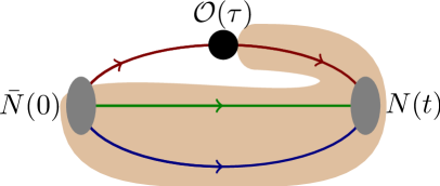
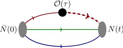
Figure 1: Diagrammatic illustration of the sequential method through the sink (left) and the stochastic method (right).

3 Assessment of the stochastic method

To test the applicability of the stochastic method, we need to determine how large $N_{S}$ must be in order to keep the stochastic noise under control. This depends on the observable of interest. To be concrete, we compute a relatively simple benchmark observable of nucleon structure, namely the nucleon axial charge $g_{A}$, using our stochastic method. This quantity can be obtained from a nucleon matrix element of the isovector axial current. For the evaluation of matrix elements of the nucleon, we need to introduce the zero momentum nucleon two-point function,

$$C_{2}^{(N)}(t) =\sum\limits_{\vec{x}}\,\mathrm{Tr}\>\left[\frac{1}{2}\left(\mathbf{1}+\gamma_{0}\right)\left\langle\mathcal{I}^{(N)}(\vec{x},t)\right.\left.\bar{\mathcal{I}}^{(N)}(0)\right\rangle\right].$$

We then examine the ratio $R_{g_{A}}$ of the nucleon three-point and two-point correlation functions,

$$R_{g_{A}}(t,\tau) =\frac{C_{3,\mathcal{O}_{k}}^{(N)}(t,\tau)}{C_{2}^{(N)}(t)}$$ (5)

$$C_{3,\mathcal{O}_{k}}^{(N)}(t,\tau;\vec{p}=\vec{p}^{\prime}=0) =\sum\limits_{\vec{x},\vec{y}}\,\mathrm{Tr}\>\left[\Gamma_{k}\left\langle\mathcal{I}^{(N)}(\vec{x},t)\right|\mathcal{O}_{k}(\vec{y},\tau)\left|\bar{\mathcal{I}}^{(N)}(0)\right\rangle\right]$$

$$\mathcal{O}_{k}\left(\vec{y},\tau\right) =\bar{u}(\vec{y},\tau)\gamma_{5}\gamma_{k}u(\vec{y},\tau)-\bar{d}(\vec{y},\tau)\gamma_{5}\gamma_{k}d(\vec{y},\tau),$$

$$\Gamma_{k} =\frac{i}{2}\left(1+\gamma_{0}\right)\gamma_{5}\gamma_{k},\quad k=1,2,3$$

In the limit of large Euclidean time separations, $R_{g_{A}}$ converges to $g_{A}$ up to the renormalization factor $Z_{A}$,

$$Z_{A}R_{g_{A}}(t,\tau) \quad\longrightarrow\quad g_{A}\quad\text{for}\quad t\to\infty,\quad\tau\to\infty\quad\text{and}\quad(t-\tau)\to\infty.$$

In this paper we use the value of the renormalization constant $Z_{A}=0.757(3)$ determined non-perturbatively [13, 14].

In order to demonstrate that the stochastic method can indeed produce results with a reasonable computational effort and is potentially competitive with the sequential method, we performed a benchmark calculation with $N_{f}=2+1+1$ flavors of quarks. We employed twisted mass fermions at maximal twist with a lattice spacing of $a\approx 0.082~{}\text{fm}$ determined from the nucleon mass [14], a pion mass of $m_{\pi}\sim 370~{}\text{MeV}$ and a volume of $L^{3}\approx(2.6~{}\text{fm})^{3}$. In Fig. 2, we show $R_{g_{A}}(t,\tau)$ obtained using the stochastic method as a function of the insertion time $\tau$ for a fixed source-sink separation $t=12a$. We compare to the value $R_{g_{A}}(t=12a,\tau=6a)$ obtained using the sequential method. For different values of $\tau$ close to the middle of the plateau the picture is similar. We use spin-color diluted random $Z(4)$ vectors as stochastic sources,

$$\eta^{a}_{\alpha}(\vec{x},t)=\delta_{a,a_{0}}\delta_{\alpha,\alpha_{0}}\delta_{t,t_{0}}\tilde{\eta}(\vec{x}),\quad a_{0}\in\{0,1,2\},\quad\alpha_{0}\in\{0,1,2,3\},\quad\tilde{\eta}(\vec{x})\in Z(4)\;.$$

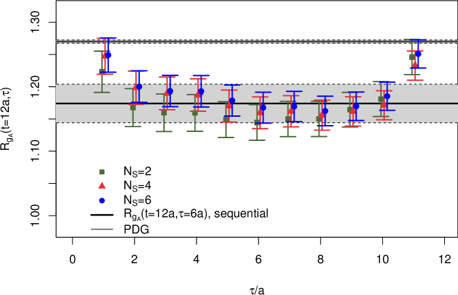
Figure 2: Plateau region of the ratio $R_{g_{A}}(t=12a,\tau)$ obtained from the stochastic method on one $N_{f}=2+1+1$ ensemble with a pion mass of $m_{\pi}\approx 370~{}\mathrm{MeV}$ and a lattice spacing $a\approx 0.082~{}\mathrm{fm}$. We use $N_{S}=2$, $4$ and $6$ spin-color diluted stochastic time-slice sources, with the source located at the sink. The source-sink separation is $12a$ and we compare to the standard sequential method, of which we show the ratio $R_{g_{A}}(t=12a,\tau=6a)$ with the light gray band. The dark gray band indicates the PDG value[15].

We have used a fixed number of gauge field configurations $N_{\text{gauge}}=460$ in both our stochastic and sequential approaches. Our observation is that using at most $N_{S}=4$ spin-color diluted stochastic noise vectors per configuration for the estimate of the all-to-all propagator is sufficient to reach the same statistical accuracy as with the sequential method.

In terms of inversions, $N_{S}=1$ corresponds to using the same number of inversions as in the sequential method i.e. ($4\times 12$) per gauge field configuration, for every additional set of stochastic sources we need ($2\times 12$) additional inversions to obtain the forward and back propagators, respectively. Thus this method would require four times more inversions. We would like to remark, however, that in the stochastic approach we can compute the correlation functions of proton and neutron without additional inversions, in contrast to the sequential method. In addition we used $3$ operators $k=1,2,3$ in Eq. (5), and correspondingly $3$ spin projectors for the stochastic method, again without the need of additional inversions when using the stochastic method. Our observation is that this procedure reduces the statistical error by about a factor $\sqrt{6}$, corresponding to a factor of about $6$ in statistics. We would like to remark however that this effective gain in statistics is rather specific for $g_{A}$ and will change for other observables.

Having demonstrated that it is in fact possible to compute $g_{A}$ using the stochastic method with a reasonable computational effort compared to the sequential method, we would like to know how the situation changes when the volume is varied. A potential danger of our stochastic method is that the number of stochastic sources required to reach the same precision as the sequential method may increase rapidly as the volume increases.

To study the volume effects, we use $N_{f}=2$ flavors of maximally twisted mass fermions, instead of the $N_{f}=2+1+1$. We expect that the stochastic noise should not noticeably depend on the number of dynamical flavors, and for the $N_{f}=2$ case, there exists a series of four different volumes at the same value of the lattice spacing, $a\approx 0.082~{}\mathrm{fm}$ [16] and a pion mass, $m_{\pi}\approx 370~{}\mathrm{MeV}$ [17]. These volumes are $V=L^{3}\times T$, where $L/a=16,20,24,32$ and the temporal extent of the lattice is $T=2L$ in all cases. This enables us to thoroughly study the volume dependence of the stochastic method over a relatively large range of spatial volumes, from about $(1.4~{}\mathrm{fm})^{3}$ to $(2.8~{}\mathrm{fm})^{3}$. This corresponds to $1.95\lessapprox m_{\pi}L\lessapprox 3.9$.

We performed an analysis using the stochastic method on a fixed number of gauge field configurations $N_{\text{gauge}}=200$ at each of the four volumes. The source-sink separation is fixed to $12a$ in all cases, which corresponds to about $1.067$ fm.

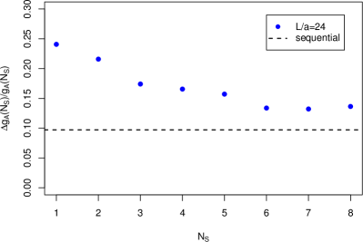
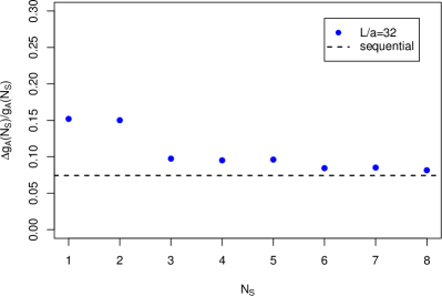
Figure 3: The filled circles show the relative error on the value obtained for $g_{A}$ as a function of the number of spin-color diluted stochastic sources $N_{S}$ per gauge field configuration. In the left panel we show results for a lattice extent of $L/a=24$ and in the right panel we show results for $L/a=32$. The dashed lines represent the error when using the sequential method. A fixed number of gauge field configurations $N_{\text{gauge}}=200$ was used, with a pion mass of $m_{\pi}\approx 370~{}\mathrm{MeV}$ and a lattice spacing of $a\approx 0.082~{}\mathrm{fm}$.

In Fig. 3 we show the relative error of $g_{A}$ as a function of the number of stochastic sources for two of the four volumes $L/a=24$ and $L/a=32$, where also the sequential method has been applied. For both volumes a convergence towards the error of the sequential method can be seen, which looks better for the larger volume, where the error is close to the error of the sequential method for $N_{S}=4$, to be conservative. This confirms the observation in the $N_{f}=2+1+1$ calculation mentioned above, which was done at about the same physical volume. The error of the error is not shown, but it is roughly of order $10\%$ of the error.

We show the combined statistical and stochastic error of $g_{A}$ obtained using the stochastic method with $N_{S}=8$ for four different volumes in Fig. 4. In order not to be subject to a systematic error we do not fit the ratio given in Eq. (5) using an estimated plateau range $\tau$ between source and sink. Instead, we take the renormalized ratio $R_{g_{A}}(t=12a,\tau=6a)$ and its error in the middle between source and sink as our estimate for $g_{A}$, where contributions from excited states are expected to be the smallest. For the larger volumes the error scales like the one of the sequential method, $V^{-0.5}$ [18]. Therefore the plot is consistent with the error being dominated by the gauge noise for larger volumes, which we have demonstrated above, see Fig. 3. Thus this method appears to work as well or even better at the larger volumes typically employed in current calculations, an observation which, of course, needs to be verified for other quantities and different physical situations.

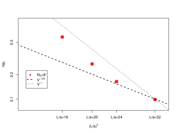
Figure 4: The filled circles show the error of $g_{A}$ using the stochastic method with a fixed number of stochastic sources $N_{S}=8$ on a fixed number of gauge fields $N_{\text{gauge}}=200$ for four different lattice sizes. The pion mass is $m_{\pi}\approx 370~{}\mathrm{MeV}$ and the lattice spacing is $a\approx 0.082~{}\mathrm{fm}$. The dashed lines indicate a scaling proportional to $V^{-1/2}$ and $V^{-1}$ and are solely meant to guide the eye. The error of the error is not much bigger than the symbol size, hence we do not show it. Please note the double logarithmic scale.

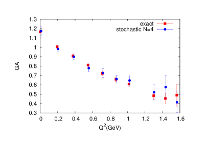
Figure 5: Comparison of $G_{A}(Q^{2})$ and $G_{p}(Q^{2})$ computed with the stochastic and standard sequential method (refered as exact in the legend). For the stochastic estimate we use a fixed number of stochastic sources $N_{S}=4$ and we use one projector for the proton correlators. The computation is performed using $N_{f}=2+1+1$ configurations fixed to $N_{\text{gauge}}=500$ with a pion mass of $m_{\pi}\approx 370~{}\mathrm{MeV}$ and a lattice spacing of $a\approx 0.082~{}\mathrm{fm}$.

The suitability of the method is demonstrated in Fig. 5 where we compare the nucleon axial form factors $G_{A}(Q^{2})$ and $G_{p}(Q^{2})$ [14] computed using the standard approach and our new method. For this comparison we use the same number of configurations and one projector. Since we use four stochatic noises diluted in colour and spin the computation is four times more expensive producing errors that are comparable to the exact case. However, the new method allows to compute the three point functions of the neutron as well as for three different projectors for free thus compensating for the increases cost. This compared with the fact that one can consider different final states e.g. a nucleon carrying momentum for free makes the new method more versatile.

4 Conclusion

We have applied a stochastic method for the calculation of nucleon matrix elements using spin-color diluted time slice sources. We have taken the case of the nucleon axial charge as a typical example of a three-point function to explore the method. Our conclusions for our test case is that the error is comparable to the error of the sequential method already at a moderate number of stochastic sources, namely four spin and color diluted timeslice stochastic sources, when using the same number of gauge field configurations. In this particular case we have effectively increased the statistics used in the stochastic method by a factor $6$ through averaging over neutron and proton correlators and using $3$ different currents, which does not require the computation of new propagators. Moreover, our results indicate that the convergence behaviour in the number of stochastic sources, $N_{S}$, appears to improve when the volume is increased.

Since the stochastic method needs of ${\cal O}(10)$ more inversions (we needed $N_{S}=4$ for $g_{A}$ but this maybe different for other matrix elements) it is competitive with the sequential method when one computes ${\cal O}(10)$ more types of matrix elements. In the case of $g_{A}$ the increase in computational effort is easily compensated by computing 6 different matrix elements with 3 different spin projections for the proton and the neutron. Thus, even with the additional computational overhead, the great versatility of the stochastic method explained in this paper outweighs the sequential method when many baryon matrix elements or form factors are computed.

References

- [1] Dru B. Renner. Status and prospects for the calculation of hadron structure from lattice QCD. PoS, LAT2009:018, 2009.
- [2] C. Alexandrou. Hadron Structure and Form Factors. PoS, LATTICE2010:001, 2010.
- [3] Kostas Orginos. Hadron interactions. PoS, LATTICE2011:016, 2011.
- [4] Constantia Alexandrou. Hadron Physics and Lattice QCD. 2012.
- [5] Simon Dinter, Constantia Alexandrou, Martha Constantinou, Vincent Drach, Karl Jansen, et al. Precision Study of Excited State Effects in Nucleon Matrix Elements. Phys.Lett., B704:89–93, 2011.
- [6] C. Alexandrou, M. Constantinou, S. Dinter, V. Drach, K. Hadjiyiannakou, et al. Sigma terms and strangeness content of the nucleon with twisted mass fermions. PoS, LATTICE2012:163, 2012.
- [7] Jeremy Green, John Negele, Andrew Pochinsky, Stefan Krieg, and Sergey Syritsyn. Excited state contamination in nucleon structure calculations. PoS, LATTICE2011:157, 2011.
- [8] Stefano Capitani, Bastian Knippschild, Michele Della Morte, and Hartmut Wittig. Systematic errors in extracting nucleon properties from lattice QCD. PoS, LATTICE2010:147, 2010.
- [9] S. Capitani, M. Della Morte, G. von Hippel, B. Jager, A. Juttner, et al. The nucleon axial charge from lattice QCD with controlled errors. Phys.Rev., D86:074502, 2012.
- [10] G. Martinelli and Christopher T. Sachrajda. A Lattice Study of Nucleon Structure. Nucl.Phys., B316:355, 1989.
- [11] Richard Evans, Gunnar Bali, and Sara Collins. Improved Semileptonic Form Factor Calculations in Lattice QCD. Phys.Rev., D82:094501, 2010.
- [12] Martin Luscher. Computational Strategies in Lattice QCD. pages 331–399, 2010.
- [13] Petros Dimopoulos et al. Renormalization constants for Wilson fermion lattice QCD with four dynamical flavours. PoS, LATTICE2010:235, 2010.
- [14] C. Alexandrou, M. Constantinou, S. Dinter, V. Drach, K. Jansen, et al. Nucleon form factors and moments of generalized parton distributions using twisted mass fermions. Phys.Rev., D88:014509, 2013.
- [15] K. Nakamura et al. Review of particle physics. J.Phys., G37:075021, 2010.
- [16] C. Alexandrou et al. Axial Nucleon form factors from lattice QCD. Phys.Rev., D83:045010, 2011.
- [17] Ph. Boucaud et al. Dynamical Twisted Mass Fermions with Light Quarks: Simulation and Analysis Details. Comput. Phys. Commun., 179:695–715, 2008.
- [18] Silas R. Beane, William Detmold, Thomas C Luu, Kostas Orginos, Assumpta Parreno, et al. High Statistics Analysis using Anisotropic Clover Lattices. II. Three-Baryon Systems. Phys.Rev., D80:074501, 2009.