Spinning particle in a varying magnetic field:

how work is done by changing external parameter

Vladimír Balek

Department of Theoretical Physics, Comenius University, Bratislava, Slovakia

The work done by a spinning particle, or on it, when put into a varying magnetic field is discussed.

If a spinning particle with magnetic moment $\mu$ is located in a magnetic field that increases from zero to $B$ and points in the direction of the moment, the particle loses energy $\mu B$. If the field behaves the same way but points in the opposite direction, the particle gains energy $\mu B$. The particle performs work $\mu B$ on the field in the former case and the field performs work $\mu B$ on the particle in the latter case. Clearly, ‘to perform work on the field’ means to perform it on the equipment generating the field, and ‘to perform work on the particle’ means to perform it on movable parts of the equipment against the action of the magnetic field of the particle. In a similar way as ‘perform work on a spinning particle’ we can ‘perform work on a weight’, if we press the spring to which the weight is attached without moving the weight itself. Work is defined as force times the distance traveled by the object on which the force is acting, hence it can be performed on a standing object only in a figurative sense; in actual fact it is performed on an intermediate system attached to the object (spring, equipment generating the field).

Work is supplied to the field or done by it also if the field is acting on a system of spinning particles in contact with heat reservoir. In this setting, the field can be viewed as an external parameter and the work can be computed from the standard formula ‘pressure times the increment of the parameter’. The ‘pressure’, however, is not the force per unit area coming from the chaotic motion of the particles, but the component of the total magnetic moment in the direction of the field. As it turns out, this quantity is related to the magnetic field in the same way as the ordinary pressure is related to the volume.

The identification of magnetic field with an external parameter, and the resulting formula for work, are well known to any student of thermodynamics. Magnetic field is mentioned on regular basis as the second example of an external parameter, the first being volume. However, to see how the work defined by the thermodynamic formula can actually be extracted from the system, that is to say, how a string of spins in a varying magnetic field can be used ’to turn the wheel’ somewhere in the equipment generating the field, we must go back to the description of magnetic field in Maxwell theory.

1. Thermodynamics of a string of spins. Consider $N$ particles with spin 1/2 and unit magnetic moment, put into homogeneous magnetic field $B$. The spins are supposed to have only two orientations, in the direction of the field (upwards) or in the direction opposite to the field (downwards). The energy of the system is

$$E=-MB,$$ (1)

with the total magnetic momentum $M$ given by

$$M=2n-N.$$ (2)

where $n$ is the number of spins oriented upwards. The entropy of the system is

$$S=\log\mbox{\Large$\left({}^{N}\mbox{\hskip-8.53581pt${}_{n}$}\right)$}.$$

(We use a system of units in which $k=1$.) For large $N$, $n$ and $N-n$ it holds

$$\mbox{\Large$\left({}^{N}\mbox{\hskip-8.53581pt${}_{n}$}\right)$}\simeq\frac{N^{N}}{\sqrt{2\pi}n^{n}(N-n)^{N-n}},$$

thus

$$S\simeq N\log N-n\log n-(N-n)\log(N-n).$$ (3)

We have omitted the constant $-\log\sqrt{2\pi}$ in the expression for $S$ since it has no effect on the results. Note that without it, $S$ assumes the correct value $S=0$ for $n=0$ and $N$. The inverse temperature can be computed from

$$\beta=\partial_{E}S=\frac{1}{2B}\partial_{n}S.$$

By inserting here the function $S(n)$ from (3), we find

$$\beta=\frac{1}{2B}\log\frac{N-n}{n}.$$ (4)

Note that we obtain the same formula when computing $\partial_{n}S$ as $\displaystyle\log\mbox{\Large$\left(\mbox{\hskip 5.69054pt${}^{N}$}\mbox{\hskip-14.22636pt${}_{n+1}$}\right)$}-\log\mbox{\Large$\left({}^{N}\mbox{\hskip-8.53581pt${}_{n}$}\right)$}$; however, we arrive at a wrong formula when using an apparently equivalent expression $\displaystyle\mbox{\Large$\left({}^{N}\mbox{\hskip-8.53581pt${}_{n}$}\right)$}^{-1}\left[\mbox{\Large$\left(\mbox{\hskip 5.69054pt${}^{N}$}\mbox{\hskip-14.22636pt${}_{n+1}$}\right)$}-\mbox{\Large$\left({}^{N}\mbox{\hskip-8.53581pt${}_{n}$}\right)$}\right]$, the reason being that one has to put $\Delta n\ll 1$ rather than $\Delta n=1$ when computing the derivative $\displaystyle\partial_{n}\mbox{\Large$\left({}^{N}\mbox{\hskip-8.53581pt${}_{n}$}\right)$}$ as the ratio of increments. (Two errors cancel each other!) From (4) we can immediately see that the temperature is positive for $n<N/2$ and negative for $n>N/2$. Having found $\beta$ as a function of $n$, we can express $n$ and, by using equations (2) and (3), $M$ and $S$, as functions of $\beta$. In this way we obtain

$$M=N\tanh\beta B$$ (5)

and, after some algebra,

$$S=-\beta MB+N\log(2\cosh\beta B).$$ (6)

The second formula can be checked by computing $S$ from the thermodynamic definition,

$$S=\int\beta\delta Q,$$

where $\delta Q$ is the heat received by the system and the integral is to be taken over a reversible process. If $B=const$, work is done neither by, nor on, the string of spins, therefore the heat received in an arbitrary process is $\delta Q=dE$. If we make use of (1) with $B=const$, we obtain

$$\delta Q=-BdM.$$ (7)

This, together with the expression (5) for $M$ (valid for systems in thermodynamic equilibrium, hence applicable to reversible processes), yields again the expression (6) for $S$.

The ‘pressure’ corresponding to the magnetic field is

$$p_{B}\equiv-(\partial_{B}E)_{S}=M,$$

where we have used the fact that $S$ can be expressed in terms of $M$ only, see equations (2) and (3). The work done by the string of spins when the magnetic field increases by $dB$ is $\delta A=p_{B}dB$, or

$$\delta A=MdB.$$ (8)

From (1) we have $dE=-MdB-BdM$, hence the expression (7) for $\delta Q$ and the recently obtained expression for $\delta A$ sum up to the first law of thermodynamics,

$$dE=-\delta A+\delta Q.$$

2. Electric charge in a varying electric field. Consider a pointlike charge $q$ in an external electric field, say, placed nearby a charged metal plate (fig. 1 to the left). Suppose

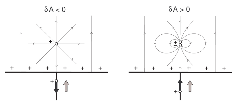
Fig. 1: Charges in a varying electric field

an additional charge $\delta Q$ is brought onto the plate from infinity, and denote the corresponding variation of the potential $\Phi$ at the point where the charge is located by $\delta\Phi$. The total work needed for this variation equals the work $\delta A_{0}$ done by the external forces that compensate the Coulomb force of the charges located on the plate, minus the work $\delta A$ done by the Coulomb forces of the charge $q$. The latter quantity can be viewed as the net energy that can be extracted from the process thanks to the fact that the charge $q$ is participating in it. Note, however, that this can be understood literally only if the positions of the charges producing the external field are not influenced by the presence of the charge $q$. If they are, as is the case for a metal plate, the work $\delta A_{0}^{\prime}$ needed to change the potential by $\delta\Phi$ when the plate is left on its own, differs in general from the work $\delta A_{0}$ needed for the same purpose when the charge $q$ is there, and the net energy gain is $\delta A_{0}+\delta A-\delta A_{0}^{\prime}$ rather than $\delta A$. Keeping in mind this reservation, let us find how $\delta A$ is related to $\delta\Phi$. Let $dQ$ be a portion of the charge $\delta Q$ transported along the path ${\bf r}={\bf r}(t)$ from the point $Q_{0}$ at infinity to the point $Q$ on the plate. The charge $q$ acts on the charge $dQ$ by the Coulomb force $d{\bf f}_{C}=dQ{\bm{\epsilon}}$, where ${\bm{\epsilon}}$ is the intensity of the electric field of the charge $q$ along the trajectory of the charge $dQ$. Thus, the work done by the charge $q$ on the charge $dQ$ is

$$dA=dQ\int\limits_{Q_{0}}^{Q}{\bm{\epsilon}}\ .\ d{\bf r}.$$

The force $d{\bf f}_{C}$ equals, by the law of action and reaction, minus the Coulomb force $d{\bf f}_{C}^{\prime}$ by which the charge $dQ$ acts on the charge $q$; that is, $d{\bf f}_{C}=-q\vec{\cal E}_{dQ}$, where $\vec{\cal E}_{dQ}$ is the intensity of the electric field of the charge $dQ$ at the point where the charge $q$ is located. Let us pass from $d{\bf f}_{C}$ to $d{\bf f}_{C}^{\prime}$, and at the same time from the path ${\bf r}={\bf r}(t)$ of the charge $dQ$, with the charge $q$ fixed at the point $P$, to the path ${\bf r}^{\prime}={\bf r}_{P}+{\bf r}_{Q}-{\bf r}(t)$ of the charge $q$, with the charge $dQ$ fixed at the point $Q$. In this way we obtain

$$dA=q\int\limits_{P_{0}}^{P}\vec{\cal E}_{dQ}\ .\ d{\bf r},$$

where the point $P_{0}$ is located at infinity symmetrically to the the point $Q_{0}$ with respect to the center of the segment $PQ$. The rewritten expression for $dA$ reduces to

$$dA=-q\Phi_{dQ}(P,Q),$$

where $\Phi_{dQ}(P,Q)$ is the potential generated at the point $P$ by the charge $dQ$ located at the point $Q$. Now, let $dQ$ be a charge that has been located on the plate from the very start, and was shifted after the charge $\delta Q$ was added to the plate. The work done on $dQ$ by $q$ can be found by rewriting the integral we have started with as

$$\int\limits_{Q_{0}}^{Q}=\int\limits_{Q_{1}}^{Q}-\int\limits_{Q_{1}}^{Q_{0}},$$

where $Q_{1}$ is an arbitrary point at infinity. If we apply the previous argument to both integrals on the right hand side, we obtain

$$dA=-q[\Phi_{dQ}(P,Q)-\Phi_{dQ}(P,Q_{0})].$$

The formulas for $dA$ can be summarized as

$$dA=-qd\Phi,$$

where $d\Phi$ is the contribution of the charge $dQ$ to the total variation of the potential $\Phi$. Finally, we sum up all contributions to the total work to obtain

$$\delta A=-q\delta\Phi.$$ (9)

With the formula for the work of a pointlike charge at hand, it is straightforward to compute the work of a dipole (fig. 1 to the right). Consider an elementary dipole with the moment $\bf d$, that is, a couple of pointlike charges $+q$ and $-q$ displaced with respect to each other by the vector $\bf a$ (so that ${\bf d}=q\bf a$), taken in the limit in which $q\to\infty$, $a\to 0$ and $qa$ is finite. With the charge $+q$ located at the point $P_{+}$ and the charge $-q$ located at the point $P_{-}$, it holds

$$\delta A=-q\delta\Phi(P_{+})+q\delta\Phi(P_{-})=-q{\bf a}\ .\ \nabla\delta\Phi,$$

and after exchanging $\nabla$ and $\delta$ and using the expression of $\bf d$ in terms of $q$ and $\bf a$, we find

$$\delta A={\bf d}\ .\ \delta\vec{\cal E},$$ (10)

where $\delta\vec{\cal E}$ is the variation of the electric intensity $\vec{\cal E}$ at the point where the dipole is located.

The two expressions for the work we have arrived at are consistent with the expressions for the potential energy of a pointlike charge

$$E=q\Phi$$ (11)

and of a dipole

$$E=-{\bf d}\ .\ \vec{\cal E}.$$ (12)

As can be seen by comparing these equations with equations (9) and (10), it holds $\delta A=-\delta E$; thus, the work done equals the energy lost.

To gain a better insight into the relation between $\delta A$ and $\delta E$, let us rederive it via the formula for the energy of electrostatic field. Consider a static, spatially bounded system of charges consisting of the subsystem $S$, generating the electric field with the potential $\Phi$ and intensity $\vec{\cal E}$, and the subsystem $s$, generating the electric field with the potential $\phi$ and intensity $\bm{\epsilon}$. The interaction energy of the two fields is

$$E_{int}=\epsilon_{0}\int\vec{\cal E}\ .\ {\bm{\epsilon}}dV,$$

and can be rewritten either as

$$E_{int}=-\epsilon_{0}\int\nabla\Phi\ .\ {\bm{\epsilon}}dV=\epsilon_{0}\int\Phi\nabla\ .\ {\bm{\epsilon}}dV=\int\Phi\rho^{(s)}dV,$$

or as

$$E_{int}=-\epsilon_{0}\int\vec{\cal E}\ .\ \nabla\phi dV=\epsilon_{0}\int\phi\nabla\ .\ \vec{\cal E}dV=\int\phi\rho^{(S)}dV,$$

where $\rho^{(s)}$ and $\rho^{(S)}$ are the charge densities of the systems $s$ and $S$ respectively. After passing to the discrete charges $Q_{I}$ (in the system $S$) and $q_{i}$ (in the system $s$), we obtain

$$E_{int}=\sum q_{i}\Phi_{i}=\sum Q_{I}\phi_{I},$$ (13)

where $\Phi_{i}$ is the value of $\Phi$ at the location of the charge $q_{i}$ and $\phi_{I}$ is the value of $\phi$ at the location of the charge $Q_{I}$. The first expression is the potential energy $E$ of the system $s$ in the field of the system $S$, and the second expression is the potential energy $E^{\prime}$ of the system $S$ in the field of the system $s$. If the system $s$ is kept fixed, like the pointlike charge and the dipole in the previous discussion, and if the charge of the system $S$ is redistributed–which may include bringing some charge from infinity to the neighborhood of the system $s$–the resulting variations of $E$ and $E^{\prime}$ coincide. Since the latter variation equals minus the work $\delta A$ done by the system $s$ on the system $S$, we arrive again at the formula $\delta A=-\delta E$.

3. Magnetic dipole in a varying magnetic field. After having analyzed the effect of a varying electric field on a pointlike charge and a dipole, let us turn to the effect of a varying magnetic field on a spinning particle. The field can be generated either by a moving magnet, or by a moving circuit, or by a circuit with a varying current. Consider first the case with the moving magnet. Let a spinning particle with the magnetic moment $\bf m$ be placed nearby a permanent magnet generating an inhomogeneous magnetic field with the induction $\bf B$ (fig. 2 to the left). After the magnet is shifted, the magnetic field at the point where the particle is located changes by $\delta\bf B$ and the particle does the work $\delta A$. The relation

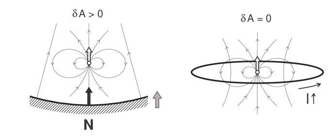
Fig. 2: Spin in a varying magnetic field

between these two quantities is most easily established with the help of the electrostatic analogy, by replacing $\bf d$ by $\bf m$ and $\vec{\cal E}$ by $\bf B$ in equation (10). In this way we obtain

$$\delta A={\bf m}\ .\ \delta{\bf B}.$$ (14)

For a string of spins that is could or could not be in contact with heat reservoir, this yields equation (8). Note that one can arrive at the expression (14) for $\delta A$ also without the reference to electrostatics. The reverse process to the one considered, with the spin moving and the magnet at rest, takes place in the Stern-Gerlach experiment. If one replaces the spinning particle by two nearby monopoles with opposite signs, one immediately obtains the well-known formula for the force acting on the particle,

$${\bf f}_{SG}={\bf m}\ .\ \nabla{\bf B}.$$

By the law of action and reaction, the particle acts on the magnet by the force ${\bf f}=-{\bf f}_{SG}$. If the magnet is moving and the spin stays at rest, the work done on the magnet is

$$\delta A={\bf f}\ .\ \delta{\bf r}={\bf f}_{SG}\ .\ \delta{\bf r}^{\prime},$$

where $\delta{\bf r}$ is the displacement of the magnet and $\delta{\bf r}^{\prime}$ is the displacement of the particle with respect to the magnet; and if we insert here the expression for ${\bf f}_{SG}$, we obtain again equation (14).

Let us now replace the magnet by the circuit. The previous reasoning seems to stay valid as long as we restrict ourselves to the circuits that move; for example, a circuit that approaches the spin without varying its shape, or a circuit that contracts towards the spin. Then, the Lorentz forces by which the spin is acting on mobile charges inside the circuit do work on the bulk of the circuit, and it turns out that the work has just the right value,

$$\delta A_{L}={\bf m}\ .\ \delta{\bf B}.$$ (15)

To check that this is the case, one needs three ingredients: the formula for the Lorentz force, the Biot-Savart law and the expression for the potential of the dipole field. We will spare ourselves this calculation since, as we will see, it can be carried out ‘in one line’ with the help of the formula for the interaction energy of the magnetic fields.

Equations (14) and (15) suggest that the behavior of a magnetic dipole in a varying field is the same as the behavior of an electric dipole in the same situation, no matter how the field is generated. However, the whole concept falls apart when the circuit neither moves as a solid body nor deforms, and the magnetic field acting on the spin changes because the current that flows through the circuit is changing (fig. 2 to the right). The Lorentz force is perpendicular to the direction of motion of the charges in the circuit, hence it does no work on them; and there is no other mechanism for doing work in sight. This casts doubts also on the previous analysis concerning the moving circuits. At a closer look we find that we have omitted an important part of the story; namely, we paid no attention to the fact that the particle generates an additional voltage in the moving circuit according to the Faraday’s law of induction. The induced voltage does work on the mobile charges in the circuit, or work must be done on the charges by the external forces in order to overcome the induced voltage; and it is a matter of simple calculation to check that this work exactly cancels the work done by the Lorentz forces. Since this result is important for further considerations, let us prove it here. Consider an electric circuit with the current $I$ in the magnetic field $\bf b$ of the spinning particle, and suppose an infinitesimal segment of the circuit $d{\bf r}$ shifts by the vector $\delta{\bf r}$, as depicted in fig. 3.

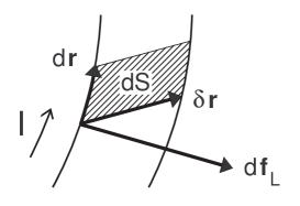
Fig. 3: Work done by the Lorentz forces

The Lorentz force acting on the segment is $d{\bf f}_{L}=Id{\bf r}\ \times\ {\bf b}$, hence the work done on the segment is

$$dA_{L}=d{\bf f}_{L}\ .\ \delta{\bf r}=I{\bf b}\ .\ (\delta{\bf r}\ \times\ d{\bf r})=I{\bf b}\ .\ d{\bf S}=Idf,$$

where $d{\bf S}$ is the element of the surface spanned by the vectors $\delta{\bf r}$ and $d{\bf r}$, and $df$ is the variation of the magnetic flux through the circuit due to the displacement of the segment. As a result, the total work done by the Lorentz forces is

$$\delta A_{L}=I\delta f,$$

where $\delta f$ is the total variation of the magnetic flux. On the other hand, the work done on the circuit by the spinning particle via electromagnetic induction is

$$\delta A_{ind}=IU_{ind}dt,$$

where $U_{ind}$ is the induced voltage in the circuit and $dt$ is the duration of the process; and since, by the Faraday’s law of induction, it holds $U_{ind}=-df/dt$, we obtain

$$\delta A_{ind}=-I\delta f.$$

As stated above, the two works cancel,

$$\delta A_{L}+\delta A_{ind}=0.$$ (16)

Note that this can be derived ‘in one line’, too, if one uses the fact that the induced electric field in the moving circuit comes from the relativistic transformation of the magnetic field into the rest frames of the elements of the circuit. To summarize, there is a sharp distinction between the case when the varying magnetic field is generated by a permanent magnet, and the case when its source is a circuit with an electric current. In the former case, the work done by the spinning particle is nonzero and given by the formula (14), while in the latter case the work is zero.

4. Energy of the magnetic dipole. The conclusion we have arrived at provokes a question about the energy balance. For a magnetic dipole in an external magnetic field, one generally uses the expression for energy analogical to that from electrostatics,

$$E=-{\bf m}\ .\ {\bf B}.$$ (17)

The previous analysis leaves an impression that the energy of the dipole equals sometimes this expression and sometimes zero. But the matters are even more mixed up. It turns out that the total energy of the dipole is actually given by equation (17) with the reversed sign,

$$E_{tot}={\bf m}\ .\ {\bf B}.$$ (18)

More precisely, this is true if the dipole as well as the source of the external magnetic field are purely classical (non-quantum) objects, since otherwise they cannot be described by the Maxwell theory in a consistent way. The requirement is obeyed neither by spinning particles like electrons or atoms, nor by permanent magnets. As we will see, these objects can be still included into the theory, but we must be cautious when doing that.

A nice derivation of $E_{tot}$, by computing the total work needed to bring an electrical circuit into a magnetic field, can be found in §15.2 of Feynman lectures. For comparison, in Jackson’s textbook the expression for $E_{tot}$ is not even written down, not to mention derived. It is only suggested, in a comment on equation (17) (on p. 185 of the 1975 edition), that $E_{tot}$ differs from $E$ because ‘in bringing the dipole $\bf m$ into its final position in the field, work must be done to keep the current $\bf J$ which produces $\bf m$ constant’. However, as the reader of Feynman knows, this is not the whole story, since work must be done also to keep the current which produces the external field constant. After computing the potential energy of a magnetic medium put into a magnetic field, Jackson comments on $E_{tot}$ again (on p. 217 of the 1975 edition), but in a rather cryptic way and as before without giving the explicit expression for it. On the contrary, the Feynman’s derivation of $E_{tot}$ is completely satisfactory and we could conclude the discussion just by giving the reference to it. However, for our purposes it is useful to compute $E_{tot}$ in a different way, as the interaction energy of fields.

Consider an elementary magnetic dipole with the moment $\bf m$, that is, a circuit with the current $i$ and the vector of the surface $\bm{\sigma}$ (so that ${\bf m}=i{\bm{\sigma}}$), taken in the limit in which $i\to\infty$, $\sigma\to 0$ and $i\sigma$ is finite. Let the dipole be put into a magnetic field generated by a system of stationary, spatially bounded currents, and denote the magnetic fields of the dipole and the currents by $\bf b$ and $\bf B$ respectively. We will show that the interaction energy of the two fields,

$$E_{int}=\frac{1}{\mu_{0}}\int{\bf B}\ .\ {\bf b}dV,$$ (19)

equals just the energy $E_{tot}$ from equation (18). Denote the distance between the dipole and the observer by $r$ and the unit vector pointing from the dipole to the observer by $\bf n$. Our starting point will be the formula for the vector potential of the dipole

$${\bf a}=\frac{\mu_{0}}{4\pi}\ \frac{{\bf m}\ \times\ {\bf n}}{r^{2}}.$$

For finite circuits, this holds only at large distances, but since we have shrunk the circuit to a point, we can write $\bf a$ in this way in the whole space. The magnetic field of the dipole is

$${\bf b}=\nabla\ \times\ {\bf a}=-\frac{\mu_{0}}{4\pi}\nabla\ \times\ \left({\bf m}\ \times\ \nabla\frac{1}{r}\right)=\frac{\mu_{0}}{4\pi}\left[({\bf m}\ .\ \nabla)\nabla\frac{1}{r}-{\bf m}\triangle\frac{1}{r}\right]=-\nabla\phi+\mu_{0}{\bf m}\delta({\bf r}),$$

where $\phi$ is the potential of the field,

$$\phi=\frac{\mu_{0}}{4\pi}\ \frac{{\bf m}\ .\ {\bf n}}{r^{2}},$$

and $\bf r$ is the radius vector of the observer with respect to the point where the dipole is located. After inserting this into $E_{int}$, we find

$$E_{int}=-\frac{1}{\mu_{0}}\int{\bf B}\ .\ \nabla\phi dV+{\bf m}\ .\ {\bf B}=\frac{1}{\mu_{0}}\int\phi\nabla\ .\ {\bf B}dV+{\bf m}\ .\ {\bf B}={\bf m}\ .\ {\bf B},$$

q. e. d.

We have argued that the dipole, disguised under the name ‘spinning particle’, does zero work in a varying magnetic field if the field is generated by electric currents. This is consistent with the fact that the dipole has a nonzero total energy which varies in the process, since the sources of the field do work on the dipole via electromagnetic induction. We have just to show that this work equals minus the variation of the energy of the dipole. To carry out the task, let us perform analogical manipulations with the formula for $E_{int}$ as in the electrostatic case. Consider a stationary, spatially bounded system of currents consisting of the subsystem $S$, generating the magnetic field with the potential $\bf A$ and intensity $\bf B$, and the subsystem $s$, generating the magnetic field with the potential $\bf a$ and intensity $\bf b$. The interaction energy of the two fields, defined in equation (19), can be rewritten as

$$E_{int}=\frac{1}{\mu_{0}}\int(\nabla\ \times\ {\bf A})\ .\ {\bf b}dV=\frac{1}{\mu_{0}}\int{\bf A}\ .\ (\nabla\ \times{\bf b})dV=\int{\bf A}\ .\ {\bf j}^{(s)}dV,$$

or as

$$E_{int}=\frac{1}{\mu_{0}}\int{\bf B}\ .\ (\nabla\ \times\ {\bf a})dV=\frac{1}{\mu_{0}}\int{\bf a}\ .\ (\nabla\ \times{\bf B})dV=\int{\bf a}\ .\ {\bf j}^{(S)}dV,$$

where ${\bf j}^{(s)}$ and ${\bf j}^{(S)}$ are the current densities of the systems $s$ and $S$ respectively. After passing to the circuits $C_{A}$ with the currents $I_{A}$ (in the system $S$) and the circuits $c_{a}$ with the currents $i_{a}$ (in the system $s$), and denoting the surfaces spanned by the circuits $C_{A}$ and $c_{a}$ by $S_{A}$ and $s_{a}$, we obtain

$$E_{int}=\sum i_{a}\oint\limits_{c_{a}}{\bf A}\ .\ d{\bf r}=\sum i_{a}\int\limits_{s_{a}}{\bf B}\ .\ d{\bf S}$$

and

$$E_{int}=\sum I_{A}\oint\limits_{C_{A}}{\bf a}\ .\ d{\bf r}=\sum I_{A}\int\limits_{S_{A}}{\bf b}\ .\ d{\bf S}.$$

In the compact notation,

$$E_{int}=\sum i_{a}F_{a}=\sum I_{A}f_{A},$$ (20)

where $F_{a}$ is the flux of $\bf B$ through the surface $s_{a}$ and $f_{A}$ is the flux of $\bf b$ through the surface $S_{A}$. The first expression can be identified with the total energy $E_{tot}$ of the system $s$ in the field of the system $S$, and the second expression can be regarded as the total energy $E_{tot}^{\prime}$ of the system $S$ in the field of the system $s$. If the system $s$ consists of one elementary dipole, the first expression yields

$$E_{int}=iF=i{\bm{\sigma}}\ .\ {\bf B}={\bf m}\ .\ {\bf B},$$

in accordance with the more direct calculation carried out above. Suppose we leave the system $s$ unchanged and change the currents, the location of the circuits and/or the shape of the circuits in the system $S$. Then, the energy of the system $s$ changes by

$$dE_{tot}=\sum i_{a}dF_{a}=-\sum i_{a}u_{ind,a}dt=-\delta a_{ind},$$

where $u_{ind,a}$ is the induced voltage in the circuit $c_{a}$, $dt$ is the duration of the process and $\delta a_{ind}$ is the total work of the voltages $u_{ind,a}$. The energy of the system $S$ changes by the same amount, $dE_{tot}^{\prime}=dE_{tot}$. To have the energy budget balanced, we must assume that the work of the induced voltage is done by the external sources on the circuit in which the voltage appears. Then, the system $S$ does the work $\delta a_{ind}$ on the system $s$, while the system $s$ does no net work on the system $S$. Indeed, if the currents are varying only, no work is done at all; and if the circuits move, the work done by the Lorentz forces is compensated by the work done by the induced voltages, see equation (16). Thus, the energies $E_{tot}$ and $E_{tot}^{\prime}$ do not change because the system $s$ does work on the system $S$, as in the electrostatic case, but because the system $S$ does work on the system $s$. This scheme has been outlined in the remark about the behavior of a dipole in a varying field we have started with; and the condition of consistency mentioned there is just the relation between $dE_{tot}$ and $\delta a_{ind}$.

To complete the analysis, let us define the mechanical energy of the system $s$ in the field of the system $S$ as $E=-E_{tot}$. Then, by mimicking the procedure by which we have obtained the relation between $dE_{tot}$ and $\delta a_{ind}$, we can obtain a relation between $dE^{\prime}$ (the variation of the mechanical energy of the system $S$ in the field of the system $s$) and $\delta A_{ind}$ (the work done on the system $S$ by the system $s$ via electromagnetic induction),

$$dE^{\prime}=\delta A_{ind}.$$

Since $\delta A_{L}=-\delta A_{ind}$, we can also write

$$dE^{\prime}=-\delta A_{L},$$

which explains the term ‘mechanical energy’ for $E$. Furthermore, from $dE=dE^{\prime}$ it follows $dE=-\delta A_{L}$; and by utilizing the expression (17) for $E$, we find the expression (15) for $\delta A_{L}$. Finally, let us consider an elementary dipole in a constant magnetic field, and discuss the variation of its energy due to the change of its orientation. To keep the notations unchanged, let us identify, as before, the dipole with the system $s$, and exchange the roles of the systems $s$ and $S$. In this way we obtain

$$dE_{tot}=-\delta A_{ind}=-\delta a_{L}-\delta a_{ind}-\delta A_{ind},$$

where the only new quantity is the work $\delta a_{L}$ done on the dipole by the external field via the Lorentz forces. If we insert here from $dE=-\delta a_{L}$, we have

$$dE_{tot}=dE-\delta a_{ind}-\delta A_{ind}.$$ (21)

The three terms on the right hand side correspond to the three contributions to $E_{tot}$ in Feynman’s §15.2. Both $\delta a_{ind}$ and $\delta A_{ind}$ equal $dE$, hence it holds $dE_{tot}=-dE$ (as it should, considering how we have defined $E$).

5. Role of quantum mechanics. Thermodynamics of a string of spins was studied in experiments with negative temperatures. The experiments used a crystal put into a strong magnetic field, with the original magnetization reversed by a discharging condenser. In principle, one could obtain the effect we are interested in by adding a permanent magnet to the setup, and moving it towards the crystal or away from it. We will not discuss how this could be done in practice; our aim is just to specify what kind of spinning particles and sources of magnetic field can be used to extract work from the field.

In the actual experiment, spinning particles were nuclei in the crystal, and in the extended version proposed here, the source would a ferromagnetic material or, in a higher resolution, ions in the domains of which the material consists. In both cases we are dealing with quantum-mechanical particles, therefore the previous reasoning about the energy balance, based on the classical Maxwell theory, must be revised. The particles are composite, so that they can occupy different energy levels in their rest frame; however, in the setting we are considering they remain all the time in the ground state. If such particle is put into a varying field or moves in a stationary field, the work $\delta a_{ind}$ is not to be included into its energy balance. The reason is obvious: even if there are electric currents inside the particle, the electromagnetic induction has no effect on them. The situation is effectively the same as with elementary particles as electron or (in the given context) nucleon. In the Maxwell theory, both kinds of particles can be modeled as tiny self-sustained electrical circuits with no response to electromagnetic induction. Elimination of the work $\delta a_{ind}$ for ions in the moving magnet leads to elimination of the work $\delta A_{ind}$ done on the magnet by the spinning particle staying at rest; and with both works $\delta a_{ind}$ and $\delta A_{ind}$ eliminated, the total energy gain from the shift of the magnet with respect to the particle equals, as desired, the work $\delta A$ of equation (14).

For composite particles that can be excited, one can argue that $\delta a_{ind}$ is still irrelevant if they just change their orientation in the external field, but can be relevant if they shift with respect to field, or stay at rest and the field varies. For the problem with a particle changing its orientation, consider how the Zeeman effect is described in QED (see, for example, Landau-Lifshitz IV, §51). In the presence of a magnetic field, the energy levels $E_{at}$ of the atom are modified by the mechanical part of the energy $E_{tot}$ only, and the energy of the emitted or absorbed photon is given by $\Delta E_{at}$, with no contribution of $\delta a_{ind}$. This is presumably the consequence of the fact that we restrict ourselves to the lowest order of perturbation theory, since then the effects of the interaction of the atom with the magnetic field and with the photon just sum up, with no interference between them. However, it seems strange to use such approximation if we know from the Maxwell theory that the work $\delta a_{ind}$ is not much less in the absolute value than the energy difference $\Delta E$, but equal to it. To remove the apparent inconsistency, let us observe that $\delta a_{ind}$ can be viewed as the energy spared by the battery that feeds the circuit, in case the induced voltage appears in the circuit and replaces a part of the emf of the battery. The energy can be turned into work, say, by using the residual emf to drive an electric motor. For a quantum-mechanical system like atom, an analogue of the battery would be an energy-supplying device taking the system back into the stationary state it occupied before, anytime it leaves it into a state with a different magnitude of magnetic moment because of spontaneous emission. Since the processes of absorbtion and emission of photons due to the Zeeman effect are well described as transitions between stationary states, the ‘battery’ is not participating in them and the work $\delta a_{ind}$ does not show up. A different question is whether the ‘battery’ should not be put into action if the system shifts in a stationary magnetic field or is located at a fixed place in a varying magnetic field. Then, the relaxation times for the transitions between the stationary states of the system are to be included into considerations.

The description of both elementary and composed particles in the Maxwell theory as self-sustained circuits seemed to work well in the previous analysis. However, if one regards electrons as truly elementary, one can ask whether they should not be represented better as ‘electric-like’ magnetic dipoles; that is, as pairs of magnetic monopoles with opposite signs placed close to each other. We mentioned this representation when motivating the formula for the Stern-Gerlach force. The two kinds of elementary dipole, the pair of monopoles and the electrical circuit, are in almost all respects undistinguishable. However, the question about the correct way how to represent electrons can still be decided experimentally; and as we will see, the answer is ‘by circuits’.

Magnetic fields of the two kinds of dipole differ only by the value they assume, in the sense of the theory of distributions, at the point where the dipole is located. If we denote the magnetic field of the monopole-based dipole by ${\bf b}_{I}$ and the magnetic field of the circuit-based dipole by ${\bf b}_{II}$, we have

$${\bf b}_{I}=-\nabla\phi,\ \ {\bf b}_{II}=-\nabla\phi+\mu_{0}{\bf m}\delta({\bf r}).$$

To be able to compare the physical effects of the two fields, we must split the vector field $\nabla\phi$, with $\phi\propto{\bf m}\ .\ {\bf n}/r^{2}$, into a regular part and a part proportional to the $\delta$-function. (A similar splitting of $\nabla\ \times\ \bf a$ is carried out in Jackson; however, the procedure presented there is restricted to the first step of our procedure.) First, consider the integral of $\nabla\phi$ over an arbitrary ball with the center at the origin, where the dipole is located. If we attempted to compute the integral directly, we would obtain an ill defined expression of the form ‘infinity times zero’, where the infinity comes from the integration over $r$ and zero comes from the integration over the angles. However, we can evaluate the integral–in fact, define it–by using the Gauss theorem, in a similar way as we evaluate the integral of the function $\triangle(1/r)$ over an arbitrary domain containing the origin. This yields

$$\int\nabla\phi dV=\oint\phi d{\bf S}=\frac{\mu_{0}}{4\pi}\oint\frac{({\bf m}\ .\ {\bf n})d{\bf S}}{r^{2}}=\mu_{0}\big{\langle}({\bf m}\ .\ {\bf n}){\bf n}\big{\rangle}=\frac{1}{3}\mu_{0}{\bf m},$$

where the angle brackets in the last but one term denote averaging over angles. Consider now a smooth spherically symmetric function $f(r)$, decreasing at infinity at least as $r^{-p}$ with some $p>0$, and compute the integral of the product $f\nabla\phi$ over the whole space. Let us divide the integration domain into two parts: the ball ${\cal B}_{\epsilon}$, with the center at the origin and the radius $\epsilon$ such that the Taylor expansion of $f$ at the origin converges uniformly in ${\cal B}_{\epsilon}$, and the rest of the space. The integral over the rest of the space, as well as the integrals of the higher order terms of the Taylor expansion in ${\cal B}_{\epsilon}$, are zero because the integral over the angles is zero and the integrals over $r$ are finite. Thus

$$\int f\nabla\phi dV=\int\limits_{{\cal B}_{\epsilon}}f\nabla\phi dV=f(0)\int\limits_{{\cal B}_{\epsilon}}\nabla\phi dV+\frac{1}{2}f^{\prime\prime}(0)\int\limits_{{\cal B}_{\epsilon}}r^{2}\nabla\phi dV+\ldots=\frac{1}{3}\mu_{0}{\bf m}f(0).$$

This suggests that we can write the vector field $\nabla\phi$ as

$$\nabla\phi=\nabla\phi_{reg}+\frac{1}{3}\mu_{0}{\bf m}\delta({\bf r}),$$

with a properly defined $\nabla\phi_{reg}$. The definition reads

$$f\nabla\phi_{reg}=[f-f_{0}(r)]\nabla\phi,$$

where $f=f({\bf r})$ is an arbitrary function of $\bf r$ and $f_{0}(r)$ is a spherically symmetric function equal to $f(0)$ at the origin and decreasing at least as $r^{-p}$ at infinity. (By subtracting $f_{0}$ from $f$ we have regularized $f$ to zero at the origin in such a way that $\nabla\phi$ weighted by the regularized function is integrable.) With the $\delta$-function term separated out from $\nabla\phi$, we can write the two versions of the dipole magnetic fields as

$${\bf b}_{I}=-\nabla\phi_{reg}-\frac{1}{3}\mu_{0}{\bf m}\delta({\bf r}),\ \ {\bf b}_{II}=-\nabla\phi_{reg}+\frac{2}{3}\mu_{0}{\bf m}\delta({\bf r}).$$ (22)

The term in the expression for the magnetic field of the electron proportional to the $\delta$-function makes all the difference when one computes the hyperfine splitting of the ground state of the hydrogen atom. The splitting produces the 21-cm hydrogen line, famous for its applications in astrophysics. By performing the computation with the fields ${\bf b}_{I}$ and ${\bf b}_{II}$, we obtain the wavelength of the transition between the split energy levels 42 cm and 21 cm, respectively. Thus, there is a strong experimental evidence that the correct choice for the magnetic field of electron is ${\bf b}_{II}$.

Acknowledgement. I am grateful to Vladimír Černý for friendly arguments about the ideas explained here.

References

Feynman R., Leighton R., Sands M.: The Feynman Lectures on Physics, Adison Wesley (1970).

Jackson J. D.: Classical Electrodynamics, John Wiley & Sons (1975).

Berestetskii V. B., Lifshitz E. M., Pitaevskii L. P.: Quantum Electrodynamics, Butterworth-Heinemann (1982).