Electronic and optical properties of Cadmium fluoride: the role of many-body effects

Abstract

Electronic excitations and optical spectra of $CdF_{2}$ are calculated up to ultraviolet employing state-of-the-art techniques based on density functional theory and many-body perturbation theory. The GW scheme proposed by Hedin has been used for the electronic self-energy to calculate single-particle excitation properties as energy bands and densities of states. For optical properties many-body effects, treated within the Bethe-Salpeter equation framework, turn out to be crucial. A bound exciton located about 1 eV below the quasiparticle gap is predicted. Within the present scheme the optical absorption spectra and other optical functions show an excellent agreement with experimental data. Moreover, we tested different schemes to obtain the best agreement with experimental data. Among the several schemes, we suggest a self-consistent quasiparticle energy scheme.

I Introduction

Fluorides and fluorite-type crystals have recently attracted much interest for their intrinsic optical properties and their potential applications in optoelectronic devices.rubloff Because of their peculiar optical properties, possible applications in ultraviolet (UV) laser optics could be considered. For example, excimer ArF lasers with an emission wavelength of 193 nm and KrF lasers with an emission wavelength of 248 nm offer many applications in medicine: e.g., photoablation of the substantia propria (or stroma of cornea), and high precision tissue ablation.medicine application This comes in addition to the common application in photolithography of the semiconductor industry.

Here we will consider cadmium fluoride ($CdF_{2}$) which is characterized by a large gap energy (of the order of 9 eV)kalugin and, hence, a high transparency in a wide energy range, while the more famous calcium fluoride ($CaF_{2}$) has a direct band gap at $\Gamma$ of $12.1$ eV and an indirect band gap estimated around $11.8$ eV.rubloff $CdF_{2}$ has been chosen as a representative candidate for a material class which seems to exhibit similar behavior, as well as numerical problems (e.g., $BaF_{2}$unpub ). In particular, its overall very small values of the dielectric function, the extended high-energy tail, and the full ionicity (i.e., the weak band dispersions) may pose critical theoretical and numerical problems.

By doping, usually with trivalent metal impurities and a certain thermochemical treatment, $CdF_{2}$ can be also produced in the semiconducting state.hayes Many dopants, as Sc and Y, generate only a shallow donor state, but In or Ga related defects exhibit a bistable behavior. In addition to the shallow state these impurity centers also possess a deep state.piekara ; dmochowski1 ; dmochowski2 Application of UV and visible light at low temperatures results in disappearance of the absorption peak corresponding to the deep electronic state and an infrared absorption band associated with the occupation of the metastable shallow state. In other words, the electrons occupying the deep state are lifted due to photoexcitation to the shallow state. At low temperatures the electrons cannot be trapped back to the deep states due to a barrier induced by different atomic configurations for shallow and deep states. The change in the electronic occupation causes a large difference in the local refractive index, which can be used as means for holographic writing at nanoscale spatial resolution.ryskin A general observation is that the formation energies of most defects are found to be very low.mattila This suggests that the fluorite structure in $CdF_{2}$ often contains high defect concentrations in agreement to what is found experimentally.hayes It is also essential that $CdF_{2}$ crystals of quite large size can be obtained at a relatively low cost.kalugin

Optical properties of $CdF_{2}$ have been experimentally determined by different spectroscopic techniques since the seventies of the previous centuryberger ; bourdillon in the fundamental absorption region and in the core-level excitation range. In the same decade reflection spectra of $CdF_{2}$ have been determined in comparison with those of $SrF_{2}$,bourdillon while UPS and XPS spectra of $CdF_{2}$ and $SrF_{2}$ have appeared in the literature in 1980.raisin Also $\beta$-$PbF_{2}$ and $CdF_{2}$ mixed crystals absorption coefficients have been reported by spectrophotometry measurements.kosacki

Various theoretical methods have been applied to study either the ground state or the excited states of the fluorite compounds. The energy bands and reflectance spectra of $CaF_{2}$ and $CdF_{2}$ have been determined within a combined tight-binding and pseudopotential method.albert Mixed crystals of $CaF_{2}$, $SrF_{2}$, $CdF_{2}$, $\beta$-$PbF_{2}$ have been studied with respect to their electronic energy bands and density of states (DOS) within the linear muffin-in orbital (LMTO) method.kudrnovsky Linear and non-linear optical properties of the cubic insulators $CaF_{2}$, $SrF_{2}$, $CdF_{2}$, $BaF_{2}$ and other compounds have been determined by first-principles orthogonalized linear combination of atomic orbitals (OLCAO).ching Point defect studies in $CdF_{2}$ have been performed within the plane wave pseudopotential (PW-PP) method.mattila With respect to one-particle and two-particle electronic properties and energy band gaps, state-of-the-art techniques have been applied until now only to $CaF_{2}$. In fact, electronic band structures of $CaF_{2}$ have been determined within a GW approximation, using a PW-PP scheme.shirley On the other hand the imaginary part $Im~{}\varepsilon(\omega)$ of the dielectric function has been calculated for $CaF_{2}$ after an iterative procedure using an effective Hamiltonian,benedict within a PW-PP scheme considering a screened interaction for electron-hole (e-h) coupling, and using localized orbitals.rohlfing

In this paper the electronic excitations and optical spectra of $CdF_{2}$ are calculated up to 40 eV employing state-of-the-art techniques based on density functional theory (DFT) and many-body perturbation theory (MBPT). We use the GW scheme proposed by Hedinhedin for the exchange-correlation (XC) self-energy, employing an Heyd-Scuseria-Ernzerhof (HSE)hse03 hybrid functional as starting point for the electronic quasiparticle structure to calculate single-particle excitation properties as the energy bands and the DOS. The DOS near the gap region and the energy-band structure are compared with existing data from literature; we show and discuss the comparison with them. The role of many-body effects turns out to be fundamental for these single-particle properties. Moreover, we demonstrate that a simple one-shot GW ($G_{0}W_{0}$) is not sufficient to obtain the correct band gaps. For optical properties excitonic effects, treated within the Bethe-Salpeter equation (BSE)onidarubioreining framework, are crucial to allow a reasonable comparison with existing experimental spectra as well. We discuss the electronic excitation structure and the optical spectra including the existence of bound excitons, and compare with available experiments.kalugin One of our goals is to provide a wide scenario of the one- and two-particle properties of this material treated within first-principles techniques. However, as considered later on, a very extended high-energy tail and overall rather small values of the dielectric function require inclusion of an unusually large number of bands or band pairs in the GW and BSE schemes. In regard to this last point, we suggest a theoretical framework and a simulative protocol able to give solutions with appreciable agreements with the available experimental measures, saving at the same time the computational demands.

II Ground state properties and computational details

All the calculations have been performed using density functional theory (DFT)kohn as implemented in the plane-wave basis code VASP.kresse ; kresse2 The projector augmented wave (PAW)paw ; paw2 method is applied to generate pseudopotentials and wave functions in the spheres around the cores. In standard use, VASP performs a fully relativistic calculation for the core-electrons and treats valence electrons in a scalar relativistic approximation.kresse ; kresse2 ; bachelet ; kaupp The effect of spin-orbit coupling on the energy bands has been considered extensively in Ref. cadelano, , where the spin-orbit effect, in the case of $CdF_{2}$, slightly decreases the gaps by about 0.05 eV only. Thus spin-orbit effects will be neglected in the present paper.

We performed the calculations using different XC functionals. The local density approximation (LDA) has been used for the XC energy, as given by Ceperley and Alder, and parametrized by Perdew and Zunger.ceperley ; perdew In addition, the generalized-gradient approximation (GGA) in the parametrization of Perdew, Burke, and Ernzerhof (PBE) is used.perdewburkeernzerhof Moreover, we considered also a revised version of the PBE functional which gives better results in solids which we shall refer to as PBEsolperdew2008 from now on.

The lattice structure of $CdF_{2}$, as well as of all the other fluorides, is a cubic one with the space group $Fm\overline{3}m$, with three ions per unit cell, i.e., one cation $Cd$ placed in the origin and two anions $F$ situated at $\pm(\frac{1}{4}a,\frac{1}{4}a,\frac{1}{4}a)$.wyckoff In the crystal the $F^{(-)}$ ions form a simple cubic sublattice surrounded by a face-centered cubic lattice of $Cd^{(++)}$ cations. All fluorides with cations belonging to the II and IIB groups are stable in this crystallographic structure.cadelano

Besides the $Cd$(5s) and $F$(2s,2p) valence states also the shallow $Cd$(4s, 4p, 4d) core states are treated as valence electrons. Inclusion of the $Cd$(4d) states is important because they appear in between the $F$(2s) and $F$(2p) bands. Inclusion of the strongly bound $Cd$(4s,4p) states (about 100 or 60 eV below the valence band maximum) is not an absolute must but helps a lot to construct s- and p-pseudopotentials with excellent scattering properties up to very high energies which are needed for a proper treatment of a large number of unoccupied bands in the calculation of the dielectric function. The wave functions are expanded in a plane-wave basis set with a cutoff energy of 950 eV. The DFT/HSE calculations for this cutoff value are fully converged. For GW/BSE calculations the error bar has been estimated at about 0.1 eV. The face-centered cubic (fcc) Brillouin zone (BZ) is sampled by $\Gamma$-point centered meshes with 16×16×16 Monkhorst-Pack k-pointsmonkhorst (converging within a few meV). The minimum of the total energy with respect to the volume is obtained by fitting to the Vinet equation of state.vinet For the calculation of the cohesive energies $E_{coh}$, we have subtracted the spin-polarized ground-state energies of the free atoms.

Table 1: Structural data for $CdF_{2}$ are given: lattice constant $a_{\circ}$, bulk modulus $B_{\circ}$ and its pressure derivative $B^{\prime}_{\circ}=dB_{\circ}/dP$, and cohesive energy $E_{coh}$. Three local and semilocal XC functionals are used, as discussed in the text. Other theoretical results and experimental references are reported in column ”OTheory” and in column ”Expt.”, respectively.

	LDA	PBE	PBEsol	OTheory	Expt.
$a_{\circ}$ (Å)	5.30	5.49	5.39	5.39kudrnovsky	5.36−5.39deligoz
$B_{\circ}$ (GPa)	126.70	93.80	108.50	123.00kudrnovsky	114.60deligoz
$B^{\prime}_{\circ}$	4.76	4.88	4.85	4.85kudrnovsky
$E_{coh}$ (eV)	-12.07	-9.55	-10.39

Comparing experimental measurementskudrnovsky with results calculated with different XC functionals, see Table 1, the best results are obtained within the PBEsol scheme. Therefore we have decided to use from now on the PBEsol lattice constant of $5.39$ Å  consistently for all calculations (ground-state, one- and two-particles excitations). This is an important point since band structure test calculations on DFT level for different lattice constants show that the gap value changes by about +0.1 eV (-0.1 eV) when going from the PBEsol to the LDA (PBE) lattice constant.

III Quasi-particle excitations

The Kohn-Sham (KS) eigenvalues of the DFT scheme cannot be interpreted as energies of single-particle/quasiparticle (QP) electronic excitations and, therefore, cannot be compared with the band structure and the DOS from experiments. We apply the many-body perturbation theory within Hedin’s GW approximation for the electronic self-energy operator.hedin It can be demonstrated that one has to solve the QP equation:hl ; onidarubioreining ; cappellinissc92 ; Stankovski

$$\left\{-\frac{\hslash^{2}}{2m_{o}}\nabla_{\mathbf{r}}^{2}+\nu_{H}(\mathbf{r})+\nu_{ext}(\mathbf{r})\right\}\Phi_{k}^{QP}(\mathbf{r})$$

$$+\int d^{3}\mathbf{r^{\prime}}\varSigma(\mathbf{r},\mathbf{r^{\prime}};\varepsilon_{k}^{QP})\Phi_{k}^{QP}(\mathbf{r^{\prime}})=\varepsilon_{k}^{QP}\Phi_{k}^{QP}(\mathbf{r}).$$ (1)

Equation (III) has a similar structure as the KS equation of DFT. The fundamental difference is that the XC potential of DFT is replaced by the non-Hermitian, nonlocal energy dependent self-energy operator $\varSigma$ resulting in QP eigenvalues $\epsilon_{k}^{QP}$ and QP wave functions $\Phi_{k}^{QP}$. Due to the fact that the Hamiltonian is non-Hermitian, QP eigenvalues are usually complex numbers. The real part describes resonance energies (excitation energies) and the imaginary part defines the lifetime of excited states. Equation (III) should be solved self-consistently; however, the most common GW approach avoids this procedure. Since empirically one often finds that QP wave functions are similar to the KS DFT-LDA ones,hl it is natural to take them as a starting point for a GW calculation and, hence, to calculate QP corrections in the sense of a perturbation treated within first-order perturbation theory.hl ; onidarubioreining ; cappellinissc92 The following equation,

$$\varepsilon_{k}^{QP}=\varepsilon_{k}+\langle\varphi_{k}\lvert\varSigma(\epsilon_{k}^{QP})-\nu_{XC}\rvert\varphi_{k}\rangle,$$ (2)

is used in conjunction with the random phase approximation (RPA) dielectric function to calculate the screened Coulomb interaction $W_{0}$ and the DFT Green’s function $G_{0}$. This approach called $G_{0}W_{0}$ usually works very well and gives very good results for the GW eigenvalues (band gaps, bandwidths and band dispersions).hl ; cappellinissc92 Another GW treatment of the QP band structure is based on the so-called generalized KS schemes (gKS).gKS1 ; gKS2 The gKS methods have in common that nonlocal exchange-correlation potentials involving partial or screened exact exchange are inserted into the KS equations combined with (semi-)local DFT potentials. From the viewpoint of band structure calculations these gKS schemes can be also considered as oversimplified GW schemes. Hence, they can be considered as an improved starting point (eigenvalues, wave functions) for $G_{0}W_{0}$ calculations. While results are similar for many systems, gKS schemes as a $G_{0}W_{0}$ starting point can provide much improved results for those cases where DFT-LDA or -GGA fails drastically (wrong band ordering, extreme gap underestimates). Since the experimental gap is almost three times as large as the DFT-PBEsol one (a gap correction of about 5 eV is necessary to arrive at the experimental values) a gKS starting point (still leaving a 3 eV gap error) can be considered as an improvement also for fluorides.

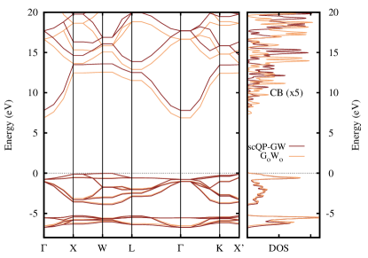
Figure 1: (Color online) Energy bands of $CdF_{2}$ calculated within the $G_{0}W_{0}$ (light lines) and the scQP-GW (dark lines) schemes. On the right panel of the figure, the DOS are reported for valence bands (VB) and conduction bands (CB). Notice the magnification factor used for the conduction bands.

In the present work QP bands of $CdF_{2}$ are determined by an iterative solution of the QP equations given in Eq.(2) with the XC self-energy in the GW approximation. The iteration starts with the gKS equations, with a self-energy derived from the nonlocal HSE03 hybrid functional (zeroth order).hse03 Subsequently, the GW corrections are calculated in first-order perturbation theory, i.e., within the one-shot $G_{0}W_{0}$. Thereby, the full frequency dependence of the RPA dielectric function entering the screened Coulomb interaction ($W_{0}$) is taken into account sampled on a frequency grid with 128 points up to $\hbar\omega\approx$350 eV, i.e., no plasmon pole modelsStankovski or model dielectric functionscappellinissc92 have been involved. We present here QP eigenvalues calculated in the $G_{0}W_{0}$ approach on top of the HSE03 ground-state electronic structures.

The strategy to calculate QP corrections then follows: The band structure and DOS have been calculated first with the PBEsol GGA, then a HSE03 calculation is performed, and finally we apply the $G_{0}W_{0}$ scheme on top of HSE03. Even after this step, the QP energies are of the order of $1$ eV smaller than the experimental ones. For comparison we made also Hartree-Fock (HF) calculations, which show as expected deviations in the opposite direction (i.e., an unrealistic overestimate of the gaps).hl ; strinati As the last step, in order to open that gap further, we performed a ”self-consistent quasiparticle energy” calculation within the GW approximation (namely, scQP-GW) which is a kind of ”iterated $G_{0}W_{0}$” just updating the eigenvalues only but keeping the HSE03 wave functions fixed. This procedure gives almost perfect gaps with respect to experiment.smith ; caruso

The main outcomes of the present paragraph are reported in Table 2 and in Figs. 1 and 2. More details are also discussed in Ref. note2, . The QP values for the fundamental gaps $\Gamma-\Gamma$ (direct) and $W-\Gamma$ (indirect) obtained within different approximations are also reported in Table 2.

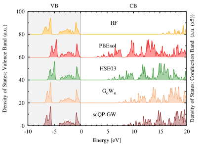
Figure 2: (Color online) Density of states around the gap region calculated within different approximations: HF, PBEsol, HSE03, $G_{0}W_{0}$, and scQP-GW. Notice the magnification factor (five) used for the conduction bands.

Table 2: QP energies for the fundamental gaps of $CdF_{2}$, between lowest CB and highest VB at high symmetry points, are computed with several approximations and compared with available experiments.

data in eV	HF	PBEsol	HSE03	$G_{0}W_{0}$	scQP-GW	Exp.
$\Gamma-\Gamma$	16.02	3.41	5.50	7.64	8.58	8.4orlowski ,8.7raisin
$W-\Gamma$	15.30	2.91	4.91	6.90	7.83	7.8orlowski

Table 3: Transition energies between lowest CB and highest VB at high symmetric points, and valence bandwidth within the two GW schemes. All data are expressed in eV.

Direct bandgaps	$G_{0}W_{0}$	scQP-GW
$L\rightarrow L$	12.11	13.08
$\Gamma\rightarrow\Gamma$	7.64	8.58
$X\rightarrow X$	12.57	13.62
$W\rightarrow W$	12.28	13.66
$K\rightarrow K$	12.65	13.44
Indirect bandgaps
$W\rightarrow\Gamma$	6.90	7.83
$W\rightarrow X$	12.50	13.55
$W\rightarrow L$	11.56	12.54
$W\rightarrow K$	12.47	13.44
VB width (F 2s - F 2p)	22.47	22.99

It is clear from Table 2 and from Figs. 1 and 2 that after the computational procedure adopted here an excellent agreement has been obtained with available experiments.orlowski ; raisin The other point is that for $CdF_{2}$, $G_{0}W_{0}$ is not sufficient and a self-consistent procedure, GW based, has to be considered in addition. Referring to Fig. 1 the main discrepancies between the different GW methods appear in the conduction bands. This point is also clear from the DOSs which are nearly overlapping for the VB energy region, as shown in Figs. 1 and 2.

Therefore, the electronic structure of $CdF_{2}$, within the PBEsol, $G_{0}W_{0}$, and scQP-GW schemes, shows an indirect gap at $W-\Gamma$ of 7.83 eV (expt. 7.8 eVorlowski ) and a larger direct gap at $\Gamma$ of 8.58 eV (expt. $8.4-8.7$ eV).orlowski ; raisin The best accordance with experiments is found within the scQP-GW scheme with a high level of accuracy. In Fig. 2 we present the calculated DOS within different schemes. As is clear from this figure the VB regions after the HSE03 and PBEsol methods seem very similar while discrepancies arise for the CB region between the results after the two methods (higher value of the gap after the HSE03 scheme).

Similarities for the VB regions appear also between the result after the $G_{0}W_{0}$ and scQP-GW schemes. The latter method does operate a further opening of the gap. In the upper part of Fig. 2, the HF DOS is reported. It determines a (too) large overestimate of the band gaps (about 16 eV at $\Gamma$) and valence bands are only partially (the shallow ones) similar to those calculated after the other methods. This HF band gap overestimate resembles a similar behavior taking place in other systems.hl ; strinati Notice that the d-electrons of $Cd$ play an important role. Indeed, they are present inside the valence bands in the energy range displayed in Fig. 1, and give rise to flat bands/sharp peaks near -5 eV, due to the localized character of these states. Localization of CB states is much weaker, and hence their dispersion is much stronger. Therefore, the average height of the DOS is smaller in comparison with the VB states. It is interesting to report in detail the energy band gaps calculated within the two different GW schemes proposed in the present publication, namely $G_{0}W_{0}$ and scQP-GW. As it is clear from Table 3 a nearly rigid shift of about 1 eV appears going from $G_{0}W_{0}$ to scQP-GW transition energies. Therefore, with respect to $CdF_{2}$, considering Fig. 1 and Table 3, the action of the self-consistency upon the eigenvalues operates a kind of ”second order scissor operator rule” on the conduction bands to obtain good accordance with experiments. The valence bandwidths after the two approximations of XC, respectively $G_{0}W_{0}$ and scQP-GW, agree within 0.5 eV. Thereby, the scQP-GW value of 22.99 eV corresponds excellently to an experimental estimate of 23 eV reported by Raisin.raisin

IV Two-particles properties and dielectric function

The treatment of excitons and resulting optical spectra, i.e., the full excitonic problem, requires to set up and diagonalize an electron-hole Hamiltonian Ĥ. Within Hedin’s GW scheme and a restriction to static screening this two-particle Hamiltonian reads for singlet excitations in matrix form as:onidarubioreining ; cappellini2

$${\hat{H}}(vc\mathbf{k},v^{\prime}c^{\prime}\mathbf{k^{\prime}})=[\varepsilon_{c}^{QP}(\mathbf{k})-\varepsilon_{v}^{QP}(\mathbf{k})]\delta_{vv^{\prime}}\delta_{cc^{\prime}}\delta_{\mathbf{k}\mathbf{k^{\prime}}}$$

$$-\int d^{3}\mathbf{r}\int d^{3}\mathbf{r^{\prime}}\varphi_{c\mathbf{k}}^{\ast}(\mathbf{r})\varphi_{c^{\prime}\mathbf{k^{\prime}}}(\mathbf{r})W(\mathbf{r},\mathbf{r^{\prime}})\varphi_{v\mathbf{k}}(\mathbf{r^{\prime}})\varphi_{v^{\prime}\mathbf{k^{\prime}}}^{\ast}(\mathbf{r^{\prime}})$$

$$+2\int d^{3}\mathbf{r}\int d^{3}\mathbf{r^{\prime}}\varphi_{c\mathbf{k}}^{\ast}(\mathbf{r})\varphi_{v\mathbf{k}}(\mathbf{r})\bar{v}(\mathbf{r},\mathbf{r^{\prime}})\varphi_{c^{\prime}\mathbf{k^{\prime}}}(\mathbf{r^{\prime}})\varphi_{v^{\prime}\mathbf{k^{\prime}}}^{\ast}(\mathbf{r^{\prime}}),$$ (3)

where matrix elements between KS or gKS wave functions of CB states and VB states occur. Contributions to Eq.(IV) which destroy particle number conservation have been omitted. The first term describes the noninteracting quasi-electron quasi-hole pairs. The second term accounts for the screened electron-hole Coulomb attraction with the statically screened Coulomb potential $W(\mathbf{r},\mathbf{r^{\prime}})$. The third contribution, governed by the nonsingular part of the bare Coulomb interaction $\bar{v}(\mathbf{r},\mathbf{r^{\prime}})$, represents the electron-hole exchange or crystal local-field effects.onidarubioreining ; roedl The QP eigenvalues entering the first term and $W(\mathbf{r},\mathbf{r^{\prime}})$ entering the second term have been directly extracted from the scQP-GW results. After diagonalization of the exciton matrix, or, more precisely, solving the homogeneous BSE or stationary two-particle Schrödinger equation with the eigenvalues $E_{\varLambda}$ and the eigenfunctions $A_{\varLambda}(vc\mathbf{k})$ of the pair states $\Lambda$, frequency dependent macroscopic dielectric function including excitonic effects can be written as:

$$\varepsilon_{\alpha\alpha}(\omega) = \delta_{\alpha\alpha}+\frac{16\pi e^{2}\hslash^{2}}{V}\sum_{\varLambda}\left\lvert\sum_{cv\mathbf{k}}\frac{\langle c\mathbf{k}\lvert v_{\alpha}\rvert v\mathbf{k}\rangle}{\varepsilon_{c}(\mathbf{k})-\varepsilon_{v}(\mathbf{k})}A_{\varLambda}(vc\mathbf{k})\right\rvert^{2}$$ (4)

$$\times \left[\frac{1}{E_{\varLambda}-\hslash(\omega+i\gamma)}+\frac{1}{E_{\varLambda}+\hslash(\omega+i\gamma)}\right]$$

where $v_{\alpha}$ is the corresponding Cartesian component of the single-particle velocity operator and $\gamma$ is the pair damping constant. The crystal volume is given by V. The details of the standard scheme using the direct diagonalization of Eq.(4) have been discussed elsewhere.onidarubioreining ; shirley ; cappellini2 ; roedl

Since the rank of the Hamilton matrix in Eq.(4) is extremely large (it is given by the number of valence bands times the number of conduction bands times the number of $\bf k$ points) a straightforward diagonalization of this matrix is often not possible due to high CPU but also memory requirements.

Therefore, we mainly refer to a numerically efficient schemesmith to solve the Bethe-Salpeter equation, which has been successfully applied by Bechstedt and coworkers on several systems. This method is based on the calculation of the time evolution of the exciton-state by Fourier transform on the time domain. This scheme delivers optical spectra directly but no exciton eigenvalues and eigenfunctions.smith The calculation of the $\omega$-dependent polarizability can be considered as an initial-value problem.smith This means that it can be written as a Fourier representation within an integral of time-dependent elements. The time evolution of these elements is driven by the pair Hamiltonian [see Eq.(IV)] and it is operatively performed by using a central-difference method, which requires one matrix-vector multiplication per time step. The time integration can be truncated due to exponential decay factors and it determines a scheme nearly independent from the dimension N (number of pair states) of the system. Two further advantages come from the matrix-vector multiplication scheme, i.e., an $O(N^{2})$ dependence on operations count and the possibility to effectively distribute the multiplications on several processors of a parallel computer.smith Applications of this method to the calculation of the $\omega$-dependent dielectric function of bulk and surface systems have been successfully performed with good comparison either with experimental results and with outcomes of the matrix diagonalization scheme. Moreover, a further speed-up of the calculations could be obtained combining this method with the use of a model dielectric function,smith ; cappellinissc92 ; cappelliniPRB93 which, however, has not been employed in the current calculations which involve no models at all. This scheme has the big advantage that it never requires the explicit diagonalization of the Hamilton matrix, because it needs only to evaluate the Hamilton exciton matrix times the current wave function for every time-step. Massive CPU-time saving and improved scaling of the computational work with respect to system size result. On the other hand, we should admit that the lack of eigenvalues and eigenfunctions limits the detailed knowledge of excitons, e.g., their real-space representation.note4

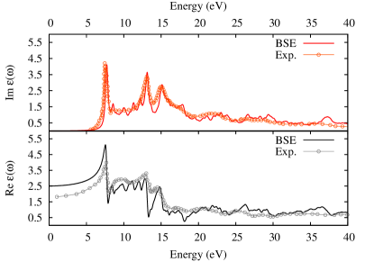
Figure 3: (Color online) Imaginary and real part of the dielectric function calculated within the BSE scheme in comparison with experimental results after Ref. bourdillon, .

The investigation of the fine structure of optical absorption spectra, especially near the absorption edge and for low energy optical transitions, requires finer k-point samplings than those necessary for the ground-state calculations. Due to the large number of bands and high cutoffs involved we have, however, to restrict ourselves to a rather limited number of k-points. For the GW and BSE calculations, we apply a $\Gamma$-centered 8×8×8 mesh. Furthermore, a sufficiently large number of conduction bands has to be included in the calculations to describe the electron-hole pair interaction properly. The number of empty states is limited by introducing a cutoff energy for the electron-hole single-particle transitions (without QP corrections) that contribute to the excitonic Hamiltonian of Eq.(IV). This transition energy cutoff was chosen to be 60 eV, corresponding to up to 50 unoccupied bands. A rank of the excitonic Hamiltonian matrix of the order of 210.000 results from this setup. In addition, for the calculation of the full frequency dependent dielectric function, screened exchange integrals, and four-orbit integrals in the GW and BSE schemes, one may introduce a lower plane-wave cutoff than for ground-state calculations without spoiling accuracy too much. In our case we use a cutoff of 475 eV.

The matrix elements of the excitonic Hamiltonian have been evaluated by means of HSE03 wave functions. Since the HSE03+$G_{0}W_{0}$ QP eigenvalues still leads to a gap underestimate (see Table 2), HSE03+$scQPGW$ eigenvalues are employed instead of HSE03+$G_{0}W_{0}$ eigenvalues on the main diagonal of the Hamiltonian. It has been carefully checked that no change of band ordering occurs when going from PBEsol to HSE03.

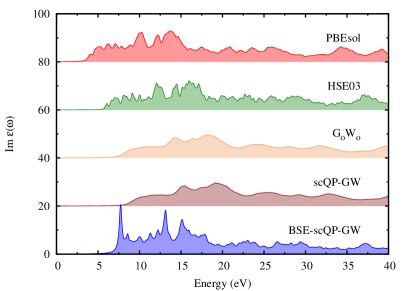
Figure 4: (Color online) Imaginary part of the macroscopic dielectric function calculated within different approximations, namely PBEsol, HSE03, $G_{0}W_{0}$, scQP-GW, and BSE. Notice that each graph has been shifted by 20 units along the y axis.

In Fig. 3, we report the principal result of the present calculations: the imaginary part of the dielectric function $Im~{}\varepsilon(\omega)$ determined within the BSE approach by using the method of Schmidt et al..smith The real part has been obtained by a Kramers-Kronig (KK) transform afterwards. Also the experimental results after Bourdillonbourdillon are reported, which are obtained with synchrotron radiation technique. The agreement both in the positions and intensities of the peaks between theory and experiment should be stressed for the imaginary part of the dielectric function (e.g., the first main three peaks are located at 7.7, 13.1, and 15.1 eV, respectively). As shown in the top panel of Fig. 3, the good agreement turns out for the full energy spectrum from near UV up to 40 eV, either below and above the QP direct gap. The first structure is a $\Gamma$ exciton, while the second and the third peaks are excitons which may originate from X, L, or W transitions between valence and conduction bands. Since we calculated the spectra directly by the method of Schmidt, we have no access to excitonic eigenvalues or eigenfunctions and can just speculate on the basis of single-QP eigenvalues.

However, on the basis of the experimental spectra of Bourdillonbourdillon as shown in Fig. 3, the value of $\varepsilon_{\infty}$ is seemingly about 1.8, which is in large discrepancy to our value of 2.5. However, one should mention that the data of Bourdillon have been extracted indirectly from reflection spectra and that there exist other values for $\varepsilon_{\infty}$ from more direct methods. Most probably, the best directly measured value is about 2.4,bosomworth and it is also indirectly confirmed by Krukowskakrukowska from measurements of the refraction index at visible optical frequencies, obtaining a value slightly larger than 2.4, i.e., about 2.46−2.5. Furthermore, by using the Lyddane-Sachs-Teller (LST) relationfox the consistency of our result could also be indirectly confirmed from measurements of $\epsilon_{0}$ (which yield values of 7.7, 7.8, and 8.3−8.5 at 0 K, 80 K, and 300 K, respectively)young together with phonon data,deligoz ; cribier which lead toward values in the range of 2.3−2.5 for $\varepsilon_{\infty}$. Hence all these values from direct measurements are in excellent agreement with our computed value. Furthermore the real part of the dielectric function $Re~{}\varepsilon(\omega)$, as shown in the second panel of Fig. 3, is in close agreement with the experimental data after Ref. bourdillon, .

In Fig. 4, we show the imaginary part of the dielectric function $Im~{}\varepsilon(\omega)$ within the different approximations proposed here, starting from the DFT reference which is the PBEsol one. Going from this approximation to the gKS HSE03 one an opening of the gap results. Both GW schemes further enlarge the gap energies. Finally the BSE results are disposed which reproduce the experiment at best in terms of oscillator strengths, peak positions, and onset behavior.

V Optical and loss functions

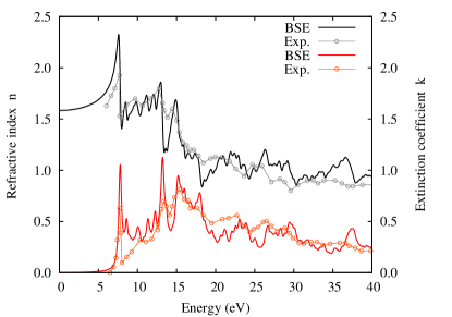
Figure 5: (Color online) Real and imaginary part of the refractive index (n,k) as a function of energy in comparison with measured spectra (after Ref. bourdillon, ).

In Fig. 5, the imaginary and real part of the refractive index in comparison with experiment after Ref. kalugin, are shown. A fair agreement results with respect to the three main peaks at 7.8, 13.2, and 15.2 eV and to the high-energy region 20−40 eV.

The reflectivity function $R$ is show in Fig. 6 in comparison with an experimental spectrumbourdillon . The positions of the main peaks of the theoretical curve (namely, occurring at 7.8 eV, 13.2 eV, and 15.2 eV) reproduce the corresponding ones of the measurement, except for the fourth peak (at 18.0 eV) which is overestimated in intensity and it should be compared with the shoulder around 17 eV as obtained in the experimental spectrum. Furthermore, the energy region above 16 eV is only in qualitative agreement with experiment. Regarding the first three peak positions of the reflectivity R, our results compare well with the experimental values after Berger and coworkers.berger Albert et al.albert assign these peaks to $\Gamma_{15}^{V}\rightarrow\Gamma_{1}^{C}$, $X_{2^{\prime}}^{V}\rightarrow X_{3}^{C}$ and $X_{5^{\prime}}^{V}\rightarrow X_{3}^{C}$ excitons. The first excitonic peak at 7.7 eV is consistent with the results of 7.6 eV given by Orlowskiorlowski , Raisinraisin , and by Formanforman and coworkers.

We focus on the fact that in our computations a natural/instrumental broadening of 0.2 eV has been applied in all the curves. Within our scheme, ”our experimental curve” is the imaginary part of the dielectric function, $Im~{}\varepsilon(\omega)$ (the first outcome of the computational code). All the other functions are derived from this calculation. Thus, an important methodological point is the following: From each optical function produced here one can return to the original dielectric function which was the output of the code we used (”our reference result”). Moreover the comparison with the experimental result for $Im~{}\varepsilon(\omega)$ is anyway excellent (see Fig. 3). If one operates a broadening to fit at best an optical function with respect to a particular experiment, the reverse operation (to generate again the $Im~{}\varepsilon(\omega)$ in agreement with experiment) is not guaranteed.

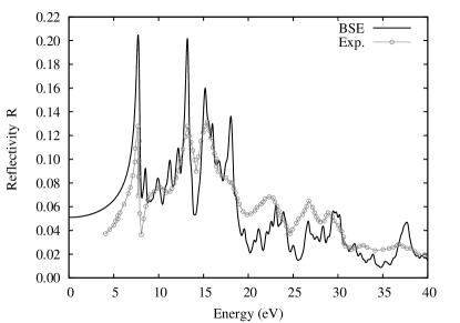
Figure 6: Calculated reflectance spectrum within BSE and experiments after Ref. bourdillon, as a function of energy.

In Fig. 7, we present the energy loss function after the present BSE calculation and experiment in a wide energy range.kalugin Also for the onset region and the main three structures below 20 eV the agreement is very close in positions and, a little less, in the oscillator strengths. For energies larger than 20 eV, a slight blue-shift of the peak positions is obtained with respect to the experimental ones. Furthermore, some differences with respect to the energy loss function $-Im~{}\varepsilon^{-1}$ of other semiconductor/insulator systems could be considered. Indeed, these systems generally show a broad single structure around the plasmon frequency $\omega_{p}$ (e.g., as in the cases of cubic GaAs and Si),cardona unlike our theoretical curve (as shown in Fig. 7), while a structure of well-separated peaks appears in the spectrum of $CdF_{2}$. A single broad structure would appear around the energy of 34.6 eV, if all the valence electrons had contributed to a single plasmonlike excitation. Instead of this hypothetic structure, only two sharp peaks (located at 7.9 and 13.4 eV, respectively) could be ascribed to excitonic effects. Analyzing the positions of the peaks above 15 eV, it seems that they occur around the energies for which the real part of the dielectric function (see Fig. 3) shows its minima; i.e., around 19 eV, 25 eV, 30 eV, and 37 eV. In particular, one could suggest that due to the distinct separation of the valence states, in the case of $CdF_{2}$ the plasmon excitations take place but divided in well-defined energy windows. One could argue that the electrons remain at disposal for collective plasmonlike excitations as far as the corresponding energies are larger than the relative binding energies. Nevertheless, this hypothesis is correct for the $F$(2p), $Cd$(4d), and $F$(2s) valence electrons but it is no more true for the $Cd$(4p) and $Cd$(4s) electrons. In fact, considering the contribution of the $F$(2p) electrons one obtains a plasmon frequency of 20.53 eV. The contribution of $F$(2p) plus $Cd$(4d) electrons gives a plasmon energy of 27.81 eV. Finally, a plasmon energy of 30.23 eV is obtained including the $F$(2s) electrons. These values are not so far away from the energies of the first three above-mentioned peaks of loss function. On the other hand, the $Cd$(4p) and $Cd$(4s) electrons lead to the following values for collective plasmonlike excitations: 32.53 eV [Cd(4p included] and 34.57 eV [Cd(4p) and $Cd$(4s) included]. These energies are much smaller than the corresponding binding energies of about -62 eV for $Cd$(4p) and -102 eV for $Cd$(4s) electrons. Therefore, a plasmonlike mechanism, involving $Cd$(4p) and $Cd$(4s) electrons, could not explain the structures in the high-energy spectrum of Fig. 7. It is interesting to note that the electron energy loss function of the rock salt rs-CdO, similarly to the present case, shows no evidence of a single pronounced plasma resonance coming from s, p or d electrons.schleife

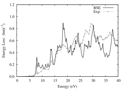
Figure 7: Electronic energy loss function after present calculation vs experiments (Ref. kalugin, ).

In Fig. 8, the absorption coefficient $\alpha$ is shown in comparison with available experimental data.kalugin Considering the first part of the $\alpha$ function, the main four sharp peaks (at 7.8 eV, 13.2 eV, 15.2 eV, and 18.0 eV) compare well with experimental data. These facts can be ascribed to the four structures of the imaginary part of the dielectric function, taking in consideration that the absorption coefficient is directly proportional to the product of $Im~{}\varepsilon(\omega)$ and the frequency, divided by the refractive index which shows a decreasing behavior in this energy range. The three broader structures in $\alpha$ at higher energies, between 20 eV and 40 eV, could be also posed in correspondence with three structures present in this energy range in the $Im~{}\varepsilon(\omega)$ curve. For these structures a slight overestimate of around 0.5−1.0 eV occurs with respect to the experimental counterpart.

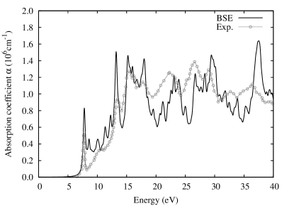
Figure 8: Absorption coefficient after present calculation vs experiment (Ref. kalugin, ).

VI CONCLUSIONS

Electronic excitations and optical properties of $CdF_{2}$ are calculated within parameter-free schemes with state-of-the-art techniques. The QP corrections within the GW approximation for the electronic self-energy of the order of 5 eV result. The $CdF_{2}$ turns out to be an indirect gap insulator with a minimum gap of 7.8 eV and a direct gap at $\Gamma$ of 8.6 eV in good accordance with experiments. The QP spectrum of $CdF_{2}$ shows similarities to the $CaF_{2}$ spectrum (i.e., direct gap of 12.1 eV and indirect gap of 11.8 eV). The Bethe-Salpeter scheme used for the optical absorption confirms the existence of an exciton located about 1.0 eV below the QP gap. The BSE spectrum for the imaginary part of the dielectric function shows an excellent accordance with experiment.

With respect to one-particle excitations we used the GW perturbative scheme for the electronic self-energy and calculated the energy bands and the DOS. The electronic density of states at the gap region for $CdF_{2}$ and the energy-band structure have been compared with existing data in literature. The role of many-body effects turns out to be important in these one-particle properties by the large opening of the energy gaps. We show, moreover, that for the optical properties, many-body effects, treated within the BSE scheme, are fundamental to obtain a reasonable comparison with existing experimental spectra. BSE imaginary part spectrum shows large differences in the shape which could not be recovered by any one-particle (GW/HSE) modified scheme at least in this material.

Finally, the existence of an exciton located 1 eV below the quasiparticle gap for this compound has been discussed.

- (1) G. W. Rubloff, Phys. Rev. B 5, 662 (1972).
- (2) J. P. Moss, B.C.M. Patel, G.J. Pearson, G. Arthur, R. A. Lawes, Biomaterials, 15, 1013 (1994).
- (3) A. I. Kalugin and V. V. Sobolev, Phys. Rev. B 71, 115112 (2005).
- (4) G. Cappellini, J. Furthmüller, E. Cadelano, and F. Bechstedt (unpublished).
- (5) R.C.N., Crystals with the Fluorite Structure - electronic, vibrational and defect properties, edited by W. Hayes (Clarendon Press, Oxford, 1974), Journal of Molecular Structure, 32, 210 (1976).
- (6) U. Piekara, J. M. Langer, B. Krukowska-Fulde, Solid State Communications, 23, 583 (1977).
- (7) J. E. Dmochowski, P. D. Wang and R. A. Stadling, Semicond. Sci. Technol. 6, 118 (1991).
- (8) J. E. Dmochowski, L. Dobaczewski, J. M. Langer and W. Jantsch , Phys. Rev. B 40, 9671 (1989).
- (9) A. I. Ryskin, A. S. Shcheulin, B. Koziarska, J. M. Langer, A. Suchocki, I. I. Buczinskaya, P. P. Fedorov, B. P. Sobolev, App. Phys. Lett., 67, 31 (1995).
- (10) T. Mattila, S. Pöykkö, R. M. Nieminen, Phys. Rev. B 56, 15665 (1997).
- (11) J.-M. Berger, G. Leveque, J. Robin, C. R. Acad. Sci. (Paris), 279, 509 (1974).
- (12) A. Bourdillon and J. Beaumont, J. Phys. C 9, L473 (1976).
- (13) C. Raisin, J. Berger, S. Robin-Kandare, G. Krill, and A. Amamou, J. Phys. C 13, 1835 (1980).
- (14) I. Kosacki and J. M. Langer, Phys. Rev. B 33, 5972 (1986).
- (15) J. P. Albert, C. Jouanin and C. Gout, Phys. Rev. B 16, 4619 (1977).
- (16) J. Kudrnovský, N. E. Christensen and J. Mašek, Phys. Rev. B 43, 12597 (1991).
- (17) W. Y. Ching, Fanqi Gan, Ming-Zhu Huang, Phys. Rev. B 52, 1596 (1995).
- (18) E. L. Shirley, Phys. Rev. B 58, 9579 (1998).
- (19) L. X. Benedict and E. L. Shirley, Phys. Rev. B 59, 5441 (1999).
- (20) Y. Ma and M. Rohlfing, Phys. Rev. B 75, 205114 (2007).
- (21) L. Hedin, Phys. Rev. 139, A796 (1965).
- (22) J. Heyd, G. E. Scuseria, and M. Ernzerhof, J. Chem. Phys. 118, 8207 (2003).
- (23) G. Onida, L. Reining, and A. Rubio, Rev. Mod. Phys. 74, 601 (2002).
- (24) W. Kohn, L. J. Sham, Phys. Rev. 140, A1133 (1965).
- (25) G. Kresse, J. Furthmüller, Comput. Mater. Sci. 6, 15 (1996).
- (26) G. Kresse, J. Furthmüller, Phys. Rev. B 54, 11169 (1996).
- (27) P. E. Blöchl, Phys. Rev. B 50, 17953 (1994).
- (28) G. Kresse, D. Joubert, Phys. Rev. B 59, 1758 (1999).
- (29) G. B. Bachelet and M. Schlüter, Phys. Rev. B 25, 2103 (1982).
- (30) M. Kaupp, and H. G. von Schnering, Inorg. Chem. 33, 4718 (1994).
- (31) E. Cadelano, G. Cappellini , Eur. Phys. J. B 81, 115-120 (2011).
- (32) D. M. Ceperley, B. J. Alder, Phys. Rev. Lett. 45, 566 (1980).
- (33) J. P. Perdew, A. Zunger, Phys. Rev. B 23, 5048 (1981).
- (34) J. P. Perdew, K. Burke, and M. Ernzerhof, Phys. Rev. Lett. 77, 3865 (1996).
- (35) J. P. Perdew, A. Ruzsinszky, G. I. Csonka, O. A. Vydrov, G. E. Scuseria, L. A. Constantin, X. Zhou, and K. Burke, Phys. Rev. Lett. 100, 136406 (2008); 102, 039902(E) (2009); A. E. Mattsson, R. Armiento, and T. R. Mattsson, ibid. 101, 239701 (2008); J. P. Perdew, A. Ruzsinszky, G. I. Csonka, O. A. Vydrov, G. E. Scuseria, L. A. Constantin, X. Zhou, and K. Burke, ibid.101, 239702 (2008).
- (36) R. W. G. Wyckoff, Crystal Structures, 9th Ed. (Interscience/John Wiley, New York 1963), Vol. 1.
- (37) H. J. Monkhort, J. D. Pack, Phys. Rev. B 13, 5188 (1976).
- (38) P. Vinet, J. H. Rose, J. Ferrante, and J. R. Smith, J. Phys.:Condens. Matter 1, 1941 (1989).
- (39) E. Deligoz, K. Colakoglu and Y.O. Ciftci, Journal of Alloys and Compounds 438, 66 (2007); D.O. Pederson and J.A. Brewer, Phys. Rev. B 16, 4546 (1977).
- (40) M. S. Hybertsen and S. G. Louie, Phys. Rev. Lett. 55, 1418 (1985); M. S. Hybertsen and S. G. Louie, Phys. Rev. B 34, 5390 (1986).
- (41) F. Bechstedt, R. Del Sole, G. Cappellini and L.Reining, Solid State Communications 84, 765 (1992).
- (42) M. Stankovski, G. Antonius, D. Waroquiers, A. Miglio, H. Dixit, K. Sankaran, M. Giantomassi, X. Gonze, M. Côté, G.-M. Rignanese, Phys. Rev. B, 84, 241201(R) (2011).
- (43) A. Seidl, A. Görling, P. Vogl, J. A. Majewski, and M. Levy, Phys. Rev. B 53, 3764 (1996).
- (44) F.Bechstedt et al., Phys. Status Solidi B 246, 1733 (2009).
- (45) G. Strinati, H. J. Mattausch, and W. Hanke, Phys. Rev. B 25, 2867 (1982).
- (46) W. G. Schmidt, S. Glutsch, P. H. Hahn, and F. Bechstedt, Phys. Rev. B 67, 085307 (2003).
- (47) F. Caruso, P. Rinke, X. Ren, M. Scheffler, A. Rubio, Phys. Rev. B 86, 081102 (2012).
- (48) For the PBEsol, and HSE03 as well, bands and DOS cutoff energies of 950 eV and 1640 eV have been used obtaining almost identical results. A reduced cutoff of 475 eV was used for the dielectric function, and screened exchange integrals. Cd (4s, 4p, 4d, 5s) and F (2s, 2p) states were included in the valence (resulting in 17 occupied bands for a 3-atom cell of , i.e., band ”17” is the valence band edge; band 1 is Cd (4s), bands 2-4 are Cd (4p), bands 5−6 are F (2s).; bands 7−11 are Cd (4d), bands 12-17 are F (2p). For GW calculations 1152 bands (1135 are unoccupied ones) and 8×8×8 k-points have been used (covering transition energies up to about 500 eV) for the evaluation of the dielectric function.
- (49) B. A. Orlowski, P. Plenkiewicz, Phys. Status Solidi B 126,285 (1984).
- (50) G. Satta, G. Cappellini, V. Olevano, L. Reining, Phys. Rev. B 70, 195212 (2004).
- (51) C. Rödl, F. Fuchs, J. Furthmüller, and F. Bechstedt, Phys. Rev. B 77, 184408 (2008).
- (52) G.Cappellini, R.Del Sole, L.Reining, F.Bechstedt, Phys. Rev. B 47, 9892 (1993).
- (53) However, due to several similarities between and we expect similar behavior also for the exciton: e.g., a Frenkel exciton as in fox with a binding energy of the order of magnitude of 1.0 eV and an exciton radius of 4−5 Å.shirley ; rohlfing ; albert
- (54) D.R. Bosomworth , Phys. Rev. 157, 709 (1967).
- (55) B. Krukowska-Fulde and T. Niemyski, J. Cryst. Growth 1, 183 (1967).
- (56) M.Fox, Optical properties of solids, (Oxford University Press, Oxford, 2001).
- (57) K.F. Young and H.P.R. Frederikse, J. Appl. Phys. 40, 3115 (1969).
- (58) D. Cribier,B. Farnoux, and B. Jacrot, Phys. Lett. 1, 187 (1962).
- (59) R.A. Forman, W.R. Hosler, and R.F. Blunt, Solid State Comm. 10, 19 (1972).
- (60) P.Y. Yu, and M.Cardona, Fundamentals of Semiconductors, Physics and Materials, (Springer-Verlag, Berlin, 2010)
- (61) A. Schleife, C. Rödl, F. Fuchs, J. Furthmüller, and F. Bechstedt, Phys. Rev. B 80, 035112 (2009)