An optimization approach to kinetic model reduction for combustion chemistry

Abstract

Model reduction methods are relevant when the computation time of a full convection–diffusion–reaction simulation based on detailed chemical reaction mechanisms is too large. In this article, we review a model reduction approach based on optimization of trajectories and show its applicability to realistic combustion models. As most model reduction methods, it identifies points on a slow invariant manifold based on time scale separation in the dynamics of the reaction system. The numerical approximation of points on the manifold is achieved by solving a semi-infinite optimization problem, where the dynamics enter the problem as constraints. The proof of existence of a solution for an arbitrarily chosen dimension of the reduced model (slow manifold) is extended to the case of realistic combustion models including thermochemistry by considering the properties of proper maps. The model reduction approach is finally applied to three models based on realistic reaction mechanisms: 1. ozone decomposition as a small test case; 2. simplified hydrogen combustion for comparison with another model reduction method; 3. syngas combustion as a test case including all features of a detailed combustion mechanism.

1 Introduction

The modeling of chemically reacting flows comprises the interplay between flow (convection), diffusion, and chemical reaction processes. This interplay is fairly complex if the model is based on a detailed combustion mechanism involving a large number of chemically reactive species and reactions. Here complexity reduction and model reduction methods can be effective tools.

A common aim of many model reduction approaches is the identification (and computation) of so called slow invariant manifolds (SIM). Many model reduction methods are applied to the chemical source term of the system of reaction transport partial differential equations (PDE), which describe the reactive flow. This means, the model reduction method is only regarding a system of ordinary differential equations (ODE) modeling the kinetic source term. Trajectories in chemical composition space are relaxing to the SIM while converging towards equilibrium. In this sense, the SIM represent the slow chemistry for a time scale separation between the tangent and normal dynamics. The existence of a SIM is closely related to multiple time scales and time scale separation and a spectral gap in the eigenvalues of the Jacobian of the chemical source term characterizes the ratio of contraction rates in tangent and normal directions.

In general, certain species will be chosen as “represented” ones for the simulation of the reacting flow based on reduced chemistry models; these are also called reaction progress variables. These variables parametrize the reduced chemistry model and for these variables the transport PDE are actually solved. The values of the remaining unrepresented variables are computed in dependence of the represented species by considering a point on the slow manifold parameterized by the reaction progress variables.

Historically, model reduction techniques have been used since the quasi steady state assumption (QSSA) and the partial equilibrium assumption (PEA) became popular—methods that had to be performed by hand Warnatz2006 . By contrast, modern model reduction methods compute a slow manifold approximation automatically without the need of expert knowledge for identification of reactions in partial equilibrium and species in steady state within a complex chemical reaction mechanism. A very popular automatic method is the intrinsic low dimensional manifold (ILDM) method, that has originally been published by Maas and Pope in Maas1992 in 1992, and its extensions. Also the computational singular perturbation (CSP) method by Lam and Goussis Lam1985 ; Lam1994 is widely applied, e.g. in Najm2010 . Another widely applied method, e.g. in Ketelheun2011 , is the method of flamelet generated manifolds Delhaye2008 . For an overview of model reduction methods, see the review Gorban2005 and the references it contains.

The scope of this manuscript is a guidance to the application of the optimization based model reduction method as introduced in Lebiedz2004c and future developments. The method is applied to chemical combustion mechanisms and results are discussed. The outline of this manuscript is as follows. In Section 2, the chemistry models regarded here are presented. The optimization problem for identification of the SIM is explained in Section 3. A short overview of appropriate numerical methods needed for solving the optimization problem is given in Section 4. Results of an application to three models are shown and discussed in Section 5.

2 Model equations in combustion chemistry

The model reduction approach discussed here is applied only to the reaction part of the reactive flow model. In this section we review knowledge that can be found in text books as e.g. Kee2003 ; Warnatz2006 .

2.1 Mass conservation laws

The general reaction transport equation in the variable $\zeta$ which can be mass fractions, temperature, or any variable describing the state of the system depending on time $t$ and space $x$ can be written as

$$\partial_{t}\zeta=\mathcal{S}(\zeta)+\mathcal{T}(\zeta,\partial_{x}\zeta,\partial_{x}^{2}\zeta),$$ (1)

where $\mathcal{S}$ is the (chemical) source term and $\mathcal{T}$ the physical transport operator, i.e. convection and diffusion.

The model comprises $n_{\mathrm{spec}}$ chemical species composed by $n_{\mathrm{elem}}$ chemical elements, and the chemical source term $\mathcal{S}$ obeys the law of elemental mass conservation and an energetic balance which will be regarded in Section 2.2. In the following, the variables $z_{i}$ are given in terms of specific moles, which are defined as the amount of species $i$ ($n_{i}$) divided by the total mass ($m$) of the system, which is the same as the species’s mass fractions ($w_{i}$) divided by its molar mass ($M_{i}$):

$$z_{i}=\frac{n_{i}}{m}=\frac{w_{i}}{M_{i}}.$$

In these variables, the mass conservation of each element in the system is formulated as

$$\bar{z}_{i}=\sum_{j=1}^{n_{\mathrm{spec}}}\chi_{ij}z_{j}\quad i=1,\dots,n_{\mathrm{elem}},$$ (2)

where $\chi_{ij}$ is the atomic composition coefficient—the number of element $i$ in species $j$. There is also a restriction to the choice of the elemental specific moles $\bar{z}_{i}$ requiring that the mass fractions sum to one

$$\sum_{i=1}^{n_{\mathrm{elem}}}\bar{M}_{i}\bar{z}_{i}=1,$$

where $\bar{M}_{i}$ is the molar mass of element $i$. This is equivalent to the conservation of the total mass of the system.

2.2 Energetic balance

Energy conservation has to be regarded, too. We consider systems within one of the four standard thermodynamic environments, i.e.

• isothermal and isochoric

• isothermal and isobaric

• adiabatic and isochoric (hence isoenergetic)

• adiabatic and isobaric (hence isenthalpic)

systems. Only the temperature is fixed in the isothermal case, while the specific enthalpy $h$

$$h=\sum_{i=1}^{n_{\mathrm{spec}}}\bar{H}_{i}^{\circ}(T)\;z_{i},$$ (3)

or the specific internal energy $e$

$$e=h-\frac{RT}{\bar{M}},$$ (4)

respectively, are fixed in the adiabatic cases, where we assume an ideal gas mixture, and $\bar{M}$ is the mean molar mass

$$\bar{M}=\frac{1}{\sum_{i=1}^{n_{\mathrm{spec}}}z_{i}}.$$

The molar enthalpy $\bar{H}_{i}^{\circ}(T)$ of species $i$ is computed by evaluation of so called NASA polynomials Burcat2005 .

2.3 Standard systems

In the optimization problem discussed later in Section 3, the dynamics of the system are considered as constraints. Therefore, the reaction ODE system that is given by the source term only is discussed in the following. This ODE system includes mass action kinetics and incorporates a differential form of the elemental mass conservation laws.

The mass balance in specific moles $z_{i}$ can be formulated as

$$\mathrm{d}_{t}z_{i}\mathrel{\mathop{:}}=\frac{\mathrm{d}}{\mathrm{d}t}z_{i}=S^{\mathrm{m}}\mathrel{\mathop{:}}=\frac{\omega}{\rho},\quad i=1,\dots,n_{\mathrm{spec}}.$$ (5)

In the right hand side of Equation (5), the symbol $\rho$ refers to the overall mass density in the system which is given via

$$\rho=\frac{m}{V}=\frac{p\bar{M}}{RT}.$$

In the isochoric case, the total mass and volume $V$ are to be known; in the isobaric case the total pressure $p$, the gas constant $R$, the temperature $T$, and the mean molar mass are necessary. The molar net chemical production rate is denoted by $\omega$ in Eq. (5). It has to be computed based on a set of chemical elementary reactions and their parameters as described in Section 2.4.

In our case, we formulate the energy balance via the right hand side of the temperature equation $\mathrm{d}_{t}T=\frac{\mathrm{d}}{\mathrm{d}t}T=S^{\mathrm{e}}$. In the isothermal case, we have $S^{\mathrm{e}}=0$ of course. In the adiabatic cases, energy or enthalpy conservation define the concise form of $S^{\mathrm{e}}$.

2.4 Chemical kinetics

In the remainder of this section, we review the computation of $\omega$. A chemical combustion mechanism generally is given as a set of $n_{\mathrm{reac}}$ elementary reactions involving $n_{\mathrm{spec}}$ species (and eventually a third body $\mathrm{M}$)

$$\sum_{i=1}^{n_{\mathrm{spec}}}\nu_{ij}^{\prime}\mathrm{X}_{i}\rightleftharpoons\sum_{i=1}^{n_{\mathrm{spec}}}\nu_{ij}^{\prime\prime}\mathrm{X}_{i},\quad j=1,\dots,n_{\mathrm{reac}}$$

with the chemical species $\mathrm{X}_{i}$ and the forward and reverse stoichiometric coefficients $\nu_{ij}^{\prime}$ and $\nu_{ij}^{\prime\prime}$. The forward and reverse rate of reaction $j$ is given via

$$r_{\mathrm{f},j} =k_{\mathrm{f},j}\prod_{i=1}^{n_{\mathrm{spec}}}c_{i}^{\nu_{ij}^{\prime}}$$ (6)

$$r_{\mathrm{r},j} =k_{\mathrm{r},j}\prod_{i=1}^{n_{\mathrm{spec}}}c_{i}^{\nu_{ij}^{\prime\prime}}$$

with the concentrations $c_{i}$ of species $i$ and the rate constants $k_{\mathrm{f},j}$ and $k_{\mathrm{r},j}$. Using the net stoichiometric coefficient

$$\nu_{ij}=\nu_{ij}^{\prime\prime}-\nu_{ij}^{\prime},$$

the net rate of change $\omega_{i}$ of species $i$ is computed as

$$\omega_{i}=\sum_{j=1}^{n_{\mathrm{reac}}}\nu_{ij}(r_{\mathrm{f},j}-r_{\mathrm{r},j}).$$ (7)

In case a third body $\mathrm{M}$ takes part in reaction $j$, third body collision efficiencies $\alpha_{i}$ for all species $i=1,\dots,n_{\mathrm{spec}}$ are to be given. The third body concentration

$$c_{\mathrm{M}}=\sum_{i=1}^{n_{\mathrm{spec}}}\alpha_{i}c_{i}$$ (8)

is then multiplied to the products in Equation (6).

Formulas for the computation of the rate coefficients are stated in the following. The elementary reactions in the mechanism considered here are given in Arrhenius format and pressure dependent Troe format, resp. The three parameters $A$, $b$, and $E_{\mathrm{a}}$ are given in the Arrhenius kinetics for each reaction. The forward reaction rate coefficient is computed via the extended Arrhenius formula

$$k_{\mathrm{f},j}=A\ T^{\tfrac{b}{1\mathrm{K}}}\ \mathrm{e}^{-\tfrac{E_{\mathrm{a}}}{RT}}.$$ (9)

A more complicated formula applies in case of pressure dependent reactions. Here $k_{\mathrm{f},j}$ is computed using Troe fall off curves Gilbert1983 ; Troe1983 . Both the low pressure rate coefficient $k_{0}$ and the high pressure coefficient $k_{\infty}$ are given via the extended Arrhenius formula (9). These are used together with a third body $\mathrm{M}$ to compute the reduced pressure

$$p_{\mathrm{r}}=\frac{k_{0}c_{\mathrm{M}}}{k_{\infty}},$$

where $c_{\mathrm{M}}$ is defined as in Equation (8). With this parameter, the final rate constant is computed as

$$k_{\mathrm{f},j}=k_{\infty}\frac{p_{\mathrm{r}}}{1+p_{\mathrm{r}}}F$$

with a function $F$. To compute the value of $F$, Gilbert, Luther, and Troe Gilbert1983 ; Troe1983 introduced the formula

$$\lg F=\left\{1+\left[\frac{\lg p_{\mathrm{r}}+c}{n-d(\lg p_{\mathrm{r}}+c)}\right]^{2}\right\}^{-1}\lg F_{\textrm{c}}$$

with a set of simplifications

$$c =-0.4-0.67\lg F_{\textrm{c}}$$

$$n =0.75-1.27\lg F_{\textrm{c}}$$

$$d =0.14$$

and the F-center-value

$$F_{\textrm{c}}=(1-a)\exp\left(-\frac{T}{T^{***}}\right)+a\exp\left(-\frac{T}{T^{*}}\right)+\exp\left(-\frac{T^{**}}{T}\right)$$

which includes the four parameters $a$, $T^{*}$, $T^{**}$, and $T^{***}$. These are given for each so called Troe-reaction.

The reverse reaction rate constant $k_{\mathrm{f},j}$ of reaction $j$ is computed via the equilibrium constant $K_{c,j}$ of the reaction. The equilibrium constant of reaction $j$ in terms of concentrations is given as

$$K_{c,j}=\left(\frac{p^{\circ}}{RT}\right)^{\nu_{j}}\exp\left(\frac{\Delta S_{\mathrm{r},j}^{\circ}}{R}-\frac{\Delta H_{\mathrm{r},j}^{\circ}}{RT}\right)$$

with the standard pressure $p^{\circ}$ and the net change of the number of species present in the gas phase

$$\nu_{j}=\sum_{i=1}^{n_{\mathrm{spec}}}\nu_{ij}.$$

The change in entropy $\Delta S_{\mathrm{r},j}$ and enthalpy $\Delta H_{\mathrm{r},j}$ can be computed by using an evaluation of the NASA polynomials for their molar values of the species involved. The reverse rate of reaction $j$ finally is

$$k_{\mathrm{r},j}=\frac{k_{\mathrm{f},j}}{K_{c,j}}.$$

3 Optimization problem

In 2004, Lebiedz introduced a model reduction method based on the minimization of entropy production rate along trajectories in chemical composition space Lebiedz2004c . The basic idea is that the SIM is characterized by maximum relaxation of the system dynamics under given constraints of fixed reaction progress variables. This approach has been extended and refined in a number of following publications Lebiedz2010a ; Lebiedz2010 ; Lebiedz2011a ; Reinhardt2008 .

The general geometric situation in the phase space of the reaction system spanned by the variables $z_{i}$ can be seen in the sketch in Figure 1. Trajectories bundle on the manifolds of slow motion, that are hierarchically ordered.

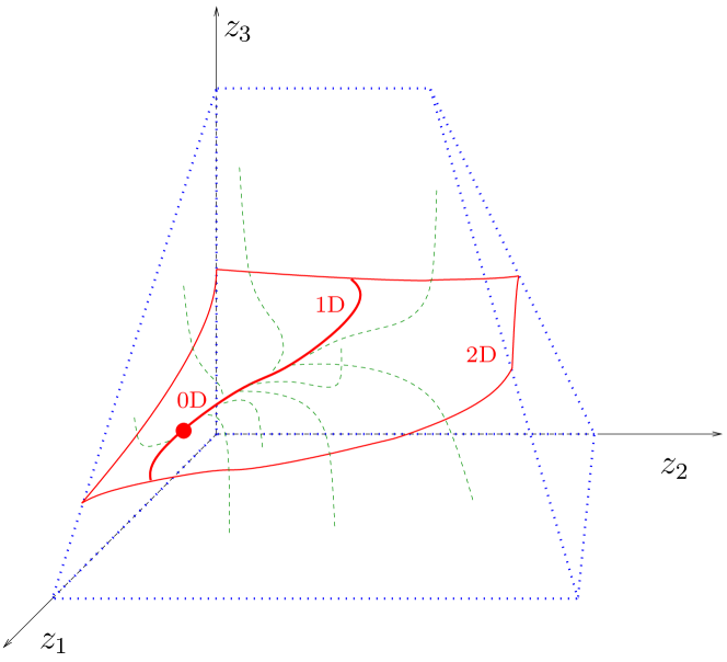
Figure 1: Sketch of the chemical composition space. The domain, where the dynamics take place is the blue-bounded polytope, here three-dimensional. Within this polytope there might be (depending on a possible time scale separation) a two-dimensional manifold (depicted in red), where (shown in green) trajectories relax onto. The trajectories relax then onto the one-dimensional manifold within the two-dimensional one. Finally the trajectories converge toward the zero-dimensional manifold: the equilibrium.

The aim is to compute an approximation of such a manifold of given dimension point-wise such that the free variables are computed depending on the given reaction progress variables which parametrize the manifold.

Following the idea of Lebiedz2004c ; Lebiedz2010a ; Lebiedz2010 ; Lebiedz2011a ; Reinhardt2008 , an optimization problem has to be solved for the approximation of points on the manifold. It can be written in specific moles and temperature as minimization of an objective functional

$$\min_{z,T}\int_{t_{0}}^{t_{\textrm{f}}}\Phi(z(t))\;\mathrm{d}t$$ (10a)

subject to

$$\mathrm{d}_{t}z(t) =S^{\mathrm{m}}(z(t),T(t))$$ (10b)

$$\mathrm{d}_{t}T(t) =S^{\mathrm{e}}(z(t),T(t))$$ (10c)

$$0 =C\left(z(t_{*}),T(t_{*})\right)$$ (10d)

$$0 =z_{j}(t_{*})-z_{j}^{t_{*}},\quad j\in\mathcal{I}_{\mathrm{rpv}}$$ (10e)

$$0 \leqslant z(t),T(t)$$ (10f)

and

$$t \in[t_{0},t_{\textrm{f}}]$$ (10g)

$$t_{*} \in[t_{0},t_{\textrm{f}}]\quad\text{(fixed)}.$$ (10h)

In the following, we explain optimization problem (10) in detail starting with the constraints.

Chemical source and heat of reaction

For the numerical solution of the optimization problem, the dynamics of the system have to be computed. The dynamics are given via the ODE system in the constraints (10b) and (10c). This ensures to identify as solution of (10) a special solution trajectory piece.

Conservation relations

All necessary additional conservation laws are combined in the (nonlinear) function $C$. As discussed before, the dynamics (10b) and (10c) contain differential forms of the balances of mass and energy. The concise values of the conserved quantities have to be specified at some (fixed) point in time along a solution which we choose to be $t_{*}$. This is Equation (2) and a specification of a fixed temperature, enthalpy, or energy, as e.g. (3) or (4), depending on the assumed thermodynamic environment.

SIM parametrization

In order to approximate the SIM, a parametrization needs to be specified. The species (i.e. the specific moles $z_{i}$) which serve as reaction progress variables and especially their number have to be specified in advance. The number of progress variables determines the chosen dimension of the SIM to be approximated.

In the case illustrated in Figure 1, one might choose $z_{1}$ and $z_{2}$ as reaction progress variables for parametrization in order to compute a value for the remaining free variable $z_{3}$ which is supposed to be on the two-dimensional manifold. Alternatively, one can choose only $z_{1}$ as reaction progress variable for approximation of the one-dimensional manifold.

The indices of the reaction progress variables are collected in the index set $\mathcal{I}_{\text{rpv}}\subset\{1,\dots,n_{\mathrm{spec}}\}$, and their values are fixed in the optimization problem to $z_{j}^{t_{*}}$.

Positivity

Since only positive values of specific moles and temperature have a physical meaning, this is included in (10f). In the optimization context with a realistic combustion mechanism included in the constraints, this is also technically important as negative values of $z_{i}$ and $T$ can result in undefined values (logarithm of a negative number) of the right hand sides $S^{\mathrm{m}}$ and $S^{\mathrm{e}}$. The positivity and the linear mass conservation relations define a polytope as depicted in Figure 1.

The chosen point in time $t_{*}\in[t_{0},t_{\mathrm{f}}]$ specifies the position where the fixation of the reaction progress variables and the constraint $C$ is applied along the trajectory piece, which is optimized. In first publications, e.g. Lebiedz2004c ; Lebiedz2010 , $t_{*}=t_{0}$ is chosen. This incorporates the demand that the trajectories are fully relaxed to the SIM at time $t_{*}$ and no further relaxation takes place afterward.

The inverse idea is the fixation at the end point $t_{*}=t_{\mathrm{f}}$. The solution point and solution trajectory piece of the optimization problem (10) is supposed to be part of the SIM. Therefore, also in backward direction of time the trajectory is supposed to be already relaxed.

This is related to the definition of positive and negative invariance of a set under a flow in dynamical systems theory.

Definition 1 (Invariant set, Wiggins1996 )

Let $\Omega\subset\mathbb{R}^{n}$ be a set. It is called invariant under the vector field $\dot{\zeta}=\mathcal{S}(\zeta)$, $\zeta\in\mathbb{R}^{n}$ if for any $\zeta_{0}\in\Omega$ it holds that $\zeta(t;\zeta_{0})\in\Omega$ for all $t\in\mathbb{R}$, where $\zeta(t;\zeta_{0})$ denotes the solution of the initial value problem $\dot{\zeta}=\mathcal{S}(\zeta)$ with initial value $\zeta_{0}$ at $t=0$. It is called positively invariant if this conditions holds for positive $t\geqslant 0$ and negatively invariant if the conditions holds for negative $t\leqslant 0$.

Clearly, the essential degrees of freedom of the optimization problem is the effective phase space dimension $n_{\mathrm{spec}}-n_{\mathrm{elem}}$ minus the number of reaction progress variables $|\mathcal{I}_{\mathrm{rpv}}|$. The goal of solving the optimization problem (10) is the determination (species reconstruction) of the “missing” values $z_{i}(t_{*}),\ i\notin\mathcal{I}_{\mathrm{rpv}}$, as a function of the parameters $z_{j}^{t_{*}},\ j\in\mathcal{I}_{\mathrm{rpv}}$.

3.1 The objective functional

The relaxation criterion $\Phi$ is supposed to measure the degree of chemical force relaxation along a trajectory. Several criteria have been tested for their SIM approximation quality, especially in Lebiedz2010 .

The SIM to be approximated is considered to be slow. This means, the residence time of the trajectory in some open neighborhood of a point on the SIM should be large—conversely the change and (to second order) the rate of change of the variable values is supposed to be small. A similar idea has been pointed out already in Girimaji1998 . The rate of change is closely related to the curvature of the trajectories as geometrical objects in phase space. The rate of change of the specific moles is simply $\dot{z}=S^{\mathrm{m}}$. Its rate of change is the second derivative

$$\ddot{z}(t)=J_{S^{\mathrm{m}}}(z(t),T(t))\;S^{\mathrm{m}}(z(t),T(t)),$$

where we denote the Jacobian of a function $S$ as $J_{S}$. This can be seen as a directional derivative of the chemical source w.r.t. its own direction $v$ which should be regarded normalized $v\mathrel{\mathop{:}}=\frac{\dot{z}}{\|\dot{z}\|_{2}}=\frac{S^{\mathrm{m}}}{\|S^{\mathrm{m}}\|_{2}}$

$$D_{v}\dot{z}(t)\mathrel{\mathop{:}}=\frac{\mathrm{d}}{\mathrm{d}\alpha}S^{\mathrm{m}}(z(t)+\alpha v,T(t))\Big{|}_{\alpha=0}=J_{S^{\mathrm{m}}}(z(t),T(t))\frac{S^{\mathrm{m}}(z(t),T(t))}{\|S^{\mathrm{m}}(z(t),T(t))\|_{2}},$$

where $\|\cdot\|_{2}$ denotes the Euclidean norm. The evaluation of this expression within the integral should be done in arc length. A re-parametrization cancels out the norm $\|S^{\mathrm{m}}(z(t),T(t))\|_{2}$ such that (in notation that coincides with the general problem (10)) a reasonable candidate for the criterion $\Phi$ would be

$$\Phi(z(t))=\|J_{S^{\mathrm{m}}}(z(t),T(t))\;S^{\mathrm{m}}(z(t),T(t))\|_{2}^{2}.$$ (11)

3.2 Solution of the optimization problem

In Lebiedz2011a , the authors study theoretical properties of the optimization based model reduction method as described in the sections before. It is shown there always exists a solution of the optimization problem (10) with only linear (mass conservation) constraints if there exists a feasible solution.

In case of a realistic combustion mechanism as a model for an adiabatic system, the nonlinear internal energy conservation or enthalpy conservation comes into play. The existence proof will be extended to this cases in the following. The crucial point is the compactness of the feasible domain, which is more complicated to ensure in the nonlinear case.

A simple way to guarantee compactness of the feasible domain would be an upper bound for the temperature. Together with the compactness argument for the linear constraints Lebiedz2011a , the compactness of the feasible domain is obvious. But it is not clear at all where to choose the upper cut off for the temperature.

We avoid this temperature cut off but make use of the definition of molar enthalpy via NASA polynomials. Thereby we accept the temperature to outrange the domain where the NASA polynomials approximate the molar enthalpy of the species appropriately.

The specific enthalpy $h$ of a system is given as

$$h=\sum_{i=1}^{n_{\mathrm{spec}}}\bar{H}_{i}^{\circ}(T)\;z_{i}.$$ (12)

The equation for the specific internal energy $e$ is

$$e=h-RT\sum_{i=1}^{n_{\mathrm{spec}}}z_{i}.$$ (13)

The molar enthalpy $\bar{H}_{i}^{\circ}(T)$ of species $i$ is a continuous function in the temperature $T$. In our case, it is computed by evaluation of the NASA polynomials. Their formula is

$$\frac{\bar{H}_{i}^{\circ}(T)}{R}=a_{6}+a_{1}T+\frac{a_{2}}{2}T^{2}+\frac{a_{3}}{3}T^{3}+\frac{a_{4}}{4}T^{4}+\frac{a_{5}}{5}T^{5}$$ (14)

with two sets of coefficients $a_{i}$, $i=1,\dots,6$. One set is given for a temperature lower than a certain switch temperature $T<T_{\mathrm{sw}}$ and one set of coefficients for high temperature $T\geqslant T_{\mathrm{sw}}$. The two branches are connected at $T_{\mathrm{sw}}$ at least continuously. There are also upper and lower bounds for the temperature, where the polynomial approximation is valid. We ignore these bounds for the following theory.

Definition 2 (Proper map, Lee2011 )

Let $X$ and $Y$ be topological spaces. A map (continuous or not) $H:X\rightarrow Y$ is called proper if the preimage $H^{-1}(K)$ of each compact subset $K\subset Y$ is compact.

To formulate a sufficient condition for properness we need the

Definition 3 (Divergence to infinity, Lee2011 )

If $X$ is a topological space, a sequence $(x_{n})$ in $X$ is said to diverge to infinity if for every compact set $K\subseteq X$ there are at most finitely many indices $n$ with element $x_{n}\in K$.

A sufficient condition for properness is the following

Lemma 1 (Properness condition, Lee2011 )

Suppose $X$ and $Y$ are topological spaces, and $H:X\rightarrow Y$ is a continuous map. If X is a second countable Hausdorff space and $F$ takes sequences diverging to infinity in $X$ to sequences diverging to infinity in $Y$, then $F$ is proper.

Proof

See (Lee2011, , p. 119).

Lemma 2 (Properness of $h$ and $e$)

The specific enthalpy $h$ and the specific internal energy $e$ defined via NASA polynomials seen as functions in $T$ and $z$ are proper maps.

Proof

The vector space $\mathbb{R}^{n_{\mathrm{spec}}+1}$ is a second countable Hausdorff space. Any non-constant polynomial takes sequences diverging to infinity in $\mathbb{R}^{n}$ equipped with its Euclidean metric induced topology to sequences diverging to infinity in $\mathbb{R}$. We can see $h$ and $e$ as polynomials of sixth degree in $z_{i}$ and $T$, see Eq. (12), (13), and (14). Therefore, $h:\mathbb{R}^{n_{\mathrm{spec}}+1}\rightarrow\mathbb{R}$ and $e:\mathbb{R}^{n_{\mathrm{spec}}+1}\rightarrow\mathbb{R}$ are proper maps.∎

Using this information, we can extend the existence lemma 2.1 in Lebiedz2011a .

Lemma 3

The feasible set at $t_{*}$

$$M=\{(z,T):C(z,T)=0;\ z_{j}-z_{j}^{t_{*}}=0,\;j\in\mathcal{I}_{\mathrm{rpv}};\ (z,T)\geqslant 0\}$$

is compact.

Proof

Case 1: isothermal combustion
The mass conservation together with the positivity and the fixed temperature define a polytope in $\mathbb{R}^{n_{\mathrm{spec}}+1}$ which is closed and bounded, hence (Heine–Borel theorem) compact.
Case 2: adiabatic combustion
As in the isothermal case, the variables $z_{i}$ are restricted to a compact polytope due to elemental mass conservation and positivity constraints. Following Lemma 2, the preimage of the singleton of the fixed energy/enthalpy is a compact subset of $\mathbb{R}^{n_{\mathrm{spec}}+1}$. This subset may only be further constrained by the polytope defined by the mass conservation and positivity, and the intersection of compact subsets is compact.∎

Lemma 4 (Existence of a solution)

If the map $\Phi:\mathbb{R}^{n_{\mathrm{spec}}}\rightarrow\mathbb{R}$ in the objective functional of the optimization problem $(\ref{eq:op})$ is a continuous function and the feasible set is not empty, there exists a solution of problem $(\ref{eq:op})$.

Proof

Following the argumentation in Lebiedz2011a , the semi-infinite optimization problem (10) can be reduced to a finite dimensional optimization problem by construction of a continuous map $(z,T)(t_{*})\mapsto\int_{t_{0}}^{t_{\textrm{f}}}\Phi\left(z(t)\right)\;\mathrm{d}t$. As seen in Lemma 3, the feasible set $M$ is compact. Therefore, existence follows from the Weierstraß theorem.∎

4 Numerical methods

The semi-infinite optimization problem (10) can be solved after suitable discretization of the ODE constraints e.g. either by a sequential quadratic programming (SQP) Powell1978 or an Interior Point (IP) method, see e.g. the review Forsgren2002 .

4.1 Discretization

In general, there are two ways for discretization and solution of (10): the sequential and the simultaneous approach.

4.1.1 Sequential approach

In the sequential approach, ODE solution and optimization are fully decoupled. The initial values $(z(t_{0}),T(t_{0}))$ are used as optimization variables. Starting at $t_{0}$, the system is integrated with a stiff ODE solver, e.g. via a backward differentiation formulae (BDF) scheme Curtiss1952 . The integrand in the objective function (10a) is integrated itself, and the end point is evaluated in sense of a Mayer term objective functional. The optimization iteration is performed after that based on the results of the integration and computed derivative information. In the cases $t_{*}=t_{0}$ and $t_{*}=t_{\mathrm{f}}$, a single shooting is appropriate as we deal with a stable ODE system; whereas in case of $t_{*}\in(t_{0},t_{\mathrm{f}})$, a double shooting is needed for the values at $t_{*}$.

4.1.2 Simultaneous approach

Sometimes (e.g. in case of unstable or extremely stiff systems), it is beneficial to use an all-at-once approach using collocation formulae Ascher1998 . In this simultaneous approach, the solution of the dynamic constraints and the optimization are coupled. The interval $[t_{0},t_{\mathrm{f}}]$ is divided into sub-intervals. Via e.g. a collocation method, polynomials are constructed on each sub-interval tangent to the vector field of the dynamics (10b) and (10c) approximating their solution, and the corresponding formulae are treated as constraints in the optimization iteration. In a collocation approach, we use a Gauß-Radau formula with linear, quadratic, and cubic polynomials, respectively, because they have stiff decay Ascher1998 .

4.2 Solution of the finite-dimensional optimization problem

In both cases (sequential and simultaneous), the result of the discretization is a finite-dimensional nonlinear programming (NLP) problem. This can be solved using an SQP algorithm or an IP method. The SQP algorithm treats the inequality constraints using an active set strategy, see e.g. Nocedal2006 . Newton’s method is applied to the first order optimality conditions of a quadratic approximation of the NLP problem including only equality and active inequality constraints. By activating and deactivating constraints, the active set in the solution is identified. In contrast in an IP method, the inequality constraints are coupled to the objective function via a barrier term forcing the iterates into the interior of the feasible domain. The resulting equality constrained NLP problem is solved with a homotopy method: Newton’s method is applied to the first order optimality conditions. In the progress of optimization, the barrier parameter is driven to zero to follow an homotopy path to the solution of the NLP problem.

4.3 Algorithms and software

In Section 5, we present results of an application of the model reduction method. We use IPOPT Waechter2006 as the main optimization tool. It turned out to be a robust IP algorithm appropriate for our problems. For the solution of linear equation systems within the optimization algorithm, HSL routines HSL2007 and MUMPS Amestoy2001 , resp., are used. Derivatives needed for the optimization are computed with the open source automatic differentiation package CppAD Bell2010 ; Bell2008 .

For discretization of the optimization problem, we use a collocation approach based on a Gauß-Radau method Ascher1998 . Alternatively, we use a shooting approach including a BDF integrator that has been developed by D. Skanda for Skanda2012 . For the numerical solution strategies, see also Lebiedz2012 . We use MATLAB for plotting.

5 Results

In this section, results for the application of the optimization based model reduction method are shown. As this manuscript is focused on the application to realistic systems, we skip a discussion of test equations for model reduction methods. These can be found in Lebiedz2010 ; Lebiedz2011a . We only consider combustion mechanisms providing the complete kinetic and thermodynamic data.

In Lebiedz2011a , it has been shown that the reverse mode ($t_{*}=t_{\mathrm{f}}$) of the method identifies the correct SIM in case of a linear test model and the Davis–Skodje test model Davis1999 , which has an analytically given one-dimensional SIM, for infinite time horizon $t_{0}\rightarrow-\infty$. Hence we use the reverse mode for all results presented here.

5.1 Ozone decomposition

As a first small test problem, we consider an ozone decomposition mechanism including only three allotropes of oxygen, namely atomic oxygen, dioxygen and ozone. The mechanism is given in Table 1.

Table 1: Ozone decomposition mechanism for the forward rates as in Maas1989 . Collision efficiencies in reactions including M: $\alpha_{\mathrm{O}}=1.14,\alpha_{\mathrm{O_{2}}}=0.40,\alpha_{\mathrm{O_{3}}}=0.92$.

Reaction			$A$ / $\textrm{cm},\textrm{mol},\textrm{s}$	$b$	$E_{\textrm{a}}$ / $\mathrm{kJ}\text{\,}{\mathrm{mol}}^{-1}$
$\mathrm{O}+\mathrm{O}+\mathrm{M}$	$\rightleftharpoons$	$\mathrm{O_{2}}+\mathrm{M}$	$2.9\times 10^{17}$	$-1.0$	$0.0$
$\mathrm{O_{3}}+\mathrm{M}$	$\rightleftharpoons$	$\mathrm{O}+\mathrm{O_{2}}+\mathrm{M}$	$9.5\times 10^{14}$	$0.0$	$95.0$
$\mathrm{O}+\mathrm{O_{3}}$	$\rightleftharpoons$	$\mathrm{O_{2}}+\mathrm{O_{2}}$	$5.2\times 10^{12}$	$0.0$	$17.4$

The thermodynamic data is used in form of NASA polynomial coefficients. In comparison to the results in Lebiedz2010 , we set up the mechanism in the framework described in Section 2. Reverse rate coefficients are derived from equilibrium thermodynamics. For mass conservation, the elemental specific mole has to be given which is

$$\bar{z}_{\mathrm{O}}=\frac{1000}{$15.999\text{\,}\mathrm{g}\text{\,}{\mathrm{mol}}^{-1}$}=$62.5\text{\,}\mathrm{mol}\text{\,}{\mathrm{kg}}^{-1}$.$$

We consider a density of $\rho=$0.2\text{\,}\mathrm{kg}\text{\,}{\mathrm{m}}^{-3}$$ in the isochoric case and a pressure of $p=${10}^{5}\text{\,}\mathrm{Pa}$$ for isobaric conditions, respectively.

In case of the ozone mechanism (Table 1), it is technically not necessary to demand positiveness of specific moles and temperature because no pressure dependent reactions are present. Therefore, the mechanism can be evaluated also in nonphysical regions (negative species concentrations visible in the plots).

Results for the four different thermodynamic environments are shown in Figure 2, 3, 4, and 5. The model has two degrees of freedom; we compute a numerical approximation of a one-dimensional SIM. The (blue) open rings in the plots are the solution points $(z,T)(t_{*})$. Orbits through these points in forward and reverse direction are also shown (blue curves), where the reverse part coincides with the optimal trajectory piece $(z,T)(t)$, $t\in[t_{0},t_{\mathrm{f}}]$. The trajectories converge toward equilibrium which is shown as full (red) dot on the left hand side of the subfigures.

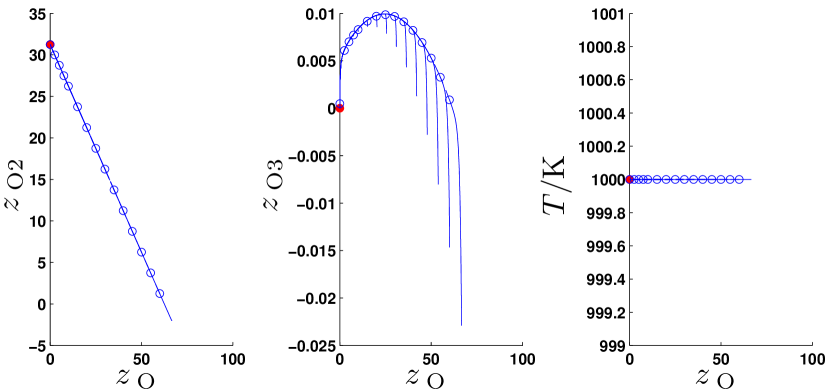
Figure 2: Results (one-dimensional SIM) for the ozone decomposition mechanism modeled within an isothermal and isochoric environment. The value of $z_{\mathrm{O}}$ serves as reaction progress variable. The optimization problem is solved several time for different values of $z_{\mathrm{O}}^{t_{*}}$ varying between zero and the largest possible value $\bar{z}_{\mathrm{O}}$. We use the reverse mode ($t_{\mathrm{f}}=t_{*}$) with an integration interval of $t_{\mathrm{f}}-t_{0}=${10}^{-6}\text{\,}\mathrm{s}$$. The free $z_{i}$ (in $\mathrm{mol}\mathrm{/}\mathrm{k}\mathrm{g}$) and temperature are plotted versus $z_{\mathrm{O}}$.

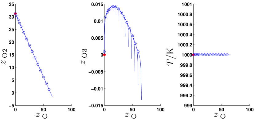
Figure 3: Results (one-dimensional SIM) for the ozone decomposition mechanism modeled within an isothermal and isobaric environment. The plot is arranged as in Figure 2. Again we use the reverse mode ($t_{\mathrm{f}}=t_{*}$) with an integration interval of $t_{\mathrm{f}}-t_{0}=${10}^{-6}\text{\,}\mathrm{s}$$.

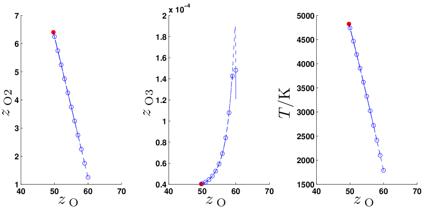
Figure 4: Results (one-dimensional SIM) for the ozone decomposition mechanism modeled within an adiabatic and isochoric environment. The plot is arranged as in Figure 2. As in the adiabatic case, the reaction evolves faster the integration horizon is reduced to $t_{\mathrm{f}}-t_{0}=${10}^{-8}\text{\,}\mathrm{s}$$.

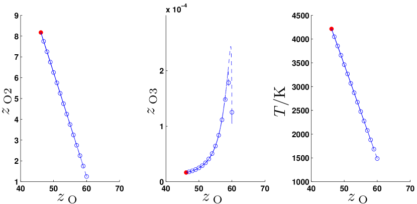
Figure 5: Results (one-dimensional SIM) for the ozone decomposition mechanism modeled within an adiabatic and isobaric environment. The plot is arranged as in Figure 2. Again the integration horizon is $t_{\mathrm{f}}-t_{0}=${10}^{-8}\text{\,}\mathrm{s}$$.

In all plots (Figure 2–5), it can be seen that near equilibrium very good results can be achieved as the SIM approximation is nearly invariant, i.e. all open dots are lying along one (slow) trajectory. But far from equilibrium at large values of the reaction progress variable $z_{\mathrm{O}}$, the full dynamics are active, so the invariance of the SIM is poor due to a lack of time scale separation. A short relaxation phase can be stated, but at least the values are in a reasonable range.

5.2 Simplified hydrogen combustion mechanism

In this section, we review a test case for a simplified combustion mechanism. The presentation and results are similar to those presented in Lebiedz2011a .

The reaction mechanism is given in Table 2. In Lebiedz2011a , we show a comparison to the results of Al-Khateeb et al. in Al-Khateeb2009 ; Al-Khateeb2010 . Hence we use the thermodynamical data (in form of NASA coefficients) we received from J. M. Powers and A. N. Al-Khateeb. The mechanism itself has been published originally in Li2004 . The simplified version shown in Table 2 has been used by Ren et al. in Ren2006a . The mechanism itself consists of five reactive species and inert nitrogen, where in comparison to a full hydrogen combustion mechanism the species $\mathrm{O}_{2}$, $\mathrm{HO}_{2}$, and $\mathrm{H}_{2}\mathrm{O}_{2}$ are removed. The species are involved in six Arrhenius type reactions, where three combination/decomposition reactions require a third body for an effective collision.

Table 2: The simplified mechanism as used in Ren2006a . Collision efficiencies $\mathrm{M}$: $\alpha_{\mathrm{H}}=1.0,\alpha_{\mathrm{H_{2}}}=2.5,\alpha_{\mathrm{OH}}=1.0$, $\alpha_{\mathrm{O}}=1.0,\alpha_{\mathrm{H_{2}O}}=12.0,\alpha_{\mathrm{N_{2}}}=1.0$.

Reaction			$A$ / ($\textrm{cm},\textrm{mol},\textrm{s}$)	$b$	$E_{\textrm{a}}$ / $\mathrm{kJ}\text{\,}{\mathrm{mol}}^{-1}$
$\mathrm{O}+\mathrm{H_{2}}$	$\rightleftharpoons$	$\mathrm{H}+\mathrm{OH}$	$5.08\times 10^{04}$	$2.7$	$26.317$
$\mathrm{H_{2}}+\mathrm{OH}$	$\rightleftharpoons$	$\mathrm{H_{2}O}+\mathrm{H}$	$2.16\times 10^{08}$	$1.5$	$14.351$
$\mathrm{O}$ + $\mathrm{H_{2}O}$	$\rightleftharpoons$	$\mathrm{2}\,\mathrm{OH}$	$2.97\times 10^{06}$	$2.0$	$56.066$
$\mathrm{H_{2}}+\mathrm{M}$	$\rightleftharpoons$	$\mathrm{2}\,\mathrm{H}+\mathrm{M}$	$4.58\times 10^{19}$	$-1.4$	$436.726$
$\mathrm{O}+\mathrm{H}+\mathrm{M}$	$\rightleftharpoons$	$\mathrm{OH}+\mathrm{M}$	$4.71\times 10^{18}$	$-1.0$	$0.000$
$\mathrm{H}+\mathrm{OH}+\mathrm{M}$	$\rightleftharpoons$	$\mathrm{H_{2}O}+\mathrm{M}$	$3.80\times 10^{22}$	$-2.0$	$0.000$

Al-Khateeb et al. identified a one-dimensional SIM for a model including this mechanism Al-Khateeb2009 . The model additionally involves the following parameters: The combustion is considered in an isothermal and isobaric environment with a temperature of $T=$3000\text{\,}\mathrm{K}$$ and a pressure of $p=$101\,325\text{\,}\mathrm{Pa}$$. The elemental mass conservation is given in terms of amount of species; it is

$$n_{\mathrm{H}}+2\,n_{\mathrm{H}_{2}}+n_{\mathrm{OH}}+2\,n_{\mathrm{H}_{2}\mathrm{O}} =$1.25\text{\times}{10}^{-3}\text{\,}\mathrm{mol}$$$

$$n_{\mathrm{OH}}+n_{\mathrm{O}}+n_{\mathrm{H}_{2}\mathrm{O}} =$4.15\text{\times}{10}^{-4}\text{\,}\mathrm{mol}$$$

$$2\,n_{\mathrm{N}_{2}} =$6.64\text{\times}{10}^{-3}\text{\,}\mathrm{mol}$.$$

Therefore, the total mass in the system is $m=$1.01\text{\times}{10}^{-4}\text{\,}\mathrm{kg}$$. We continue to use the specific moles as our standard variables here and use $z_{i}=\tfrac{n_{i}}{m}$ in the following.

The results are shown in Figure 6. There is a very good agreement of our results with theirs. Even on both sides of equilibrium, our approximations coincide with the correct one-dimensional SIM on its both branches which consist of two heteroclinic orbits in this case.

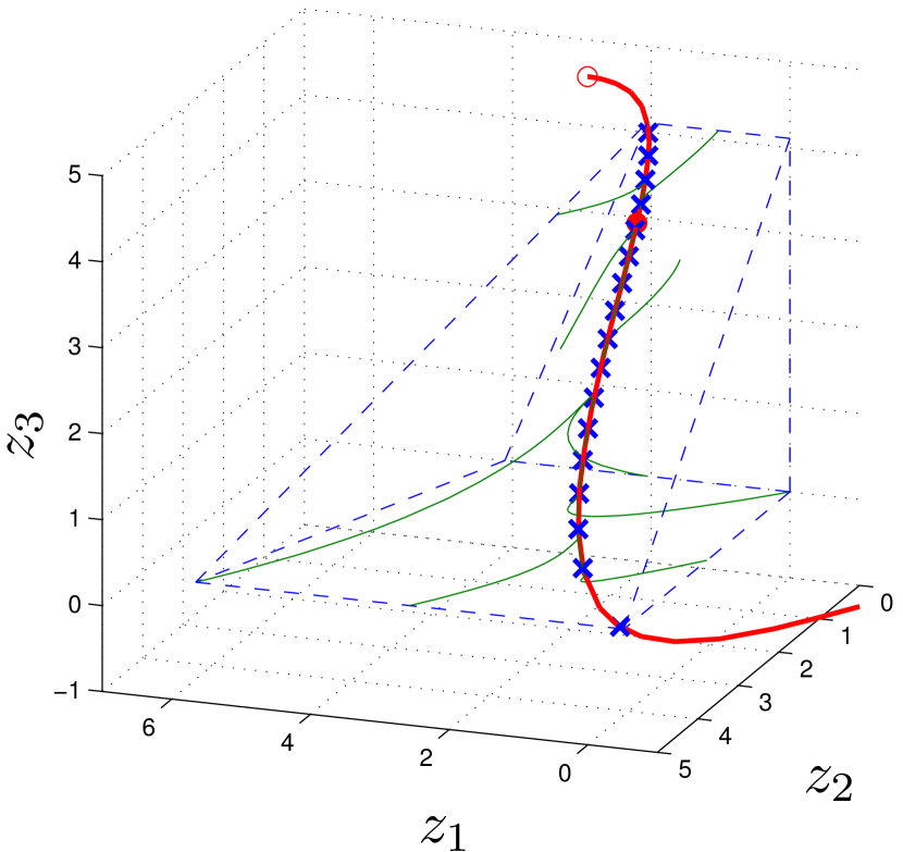
Figure 6: Three-dimensional plot of the results for the numerical approximation of a one-dimensional SIM of the simplified combustion mechanism computed with the reverse mode, $z_{\mathrm{H}_{2}\mathrm{O}}$ as reaction progress variable, and $t_{\mathrm{f}}-t_{0}=${10}^{-7}\text{\,}\mathrm{s}$$. The illustration is similar to Figure 9 in Al-Khateeb2009 . The blue bounded polytope shows the physically feasible state space. Green curves correspond to some “arbitrary” trajectories for illustration. The red curve depicts the two branches of the SIM as derived in Al-Khateeb2009 . The open red dot represents the unstable fixed point ($R_{6}$ in Al-Khateeb2009 ); the full red dot represents the equilibrium ($R_{7}$). Our results are included as blue crosses. The state of the species is given as $z_{1}=z_{\mathrm{H}_{2}}$, $z_{2}=z_{\mathrm{O}}$, and $z_{3}=z_{\mathrm{H}_{2}\mathrm{O}}$ in $\mathrm{mol}\text{\,}{\mathrm{kg}}^{-1}$.

5.3 Syngas combustion mechanism

As a last example of a full detailed chemistry combustion mechanism, we use a syngas combustion extracted from the GRI 3.0 mechanism Smith1999 . It consists of all 33 reactions of the GRI 3.0 mechanism which involve no other species than $\mathrm{O}$, $\mathrm{O}_{2}$, $\mathrm{H}$, $\mathrm{OH}$, $\mathrm{H}_{2}$, $\mathrm{HO}_{2}$, $\mathrm{H}_{2}\mathrm{O}_{2}$, $\mathrm{H}_{2}\mathrm{O}$, $\mathrm{N}_{2}$, $\mathrm{CO}$, and $\mathrm{CO}_{2}$. Those 33 reactions can be split up into 31 Arrhenius-type and two pressure-dependent ones.

The overall reaction can be stated as

$$\mathrm{H}_{2}+\mathrm{CO}+\mathrm{O}_{2}\rightarrow\mathrm{H}_{2}\mathrm{O}+\mathrm{CO}_{2},$$

where $\mathrm{N}_{2}$ only serves as a collision partner. We assume a stoichiometric mixture of syngas with air in an adiabatic and isochoric environment. As fixed mass density, we use $\rho=$0.3\text{\,}\mathrm{kg}\text{\,}{\mathrm{m}}^{-3}$$. We assume a ratio of $n_{\mathrm{H}_{2}}:n_{\mathrm{CO}}=1:1$, and a ratio of $n_{\mathrm{O}_{2}}:n_{\mathrm{N}_{2}}=1:3.76$. This leads to a unburned mixture of $z_{\mathrm{CO}}=z_{\mathrm{H}_{2}}=$5.973\text{\,}\mathrm{mol}\text{\,}{\mathrm{kg}}^{-1}$$ and $z_{\mathrm{N}_{2}}=$22.46\text{\,}\mathrm{mol}\text{\,}{\mathrm{kg}}^{-1}$$. The specific internal energy of this mixture at a temperature of $T=$1000\text{\,}\mathrm{K}$$ is used as a fixed specific internal energy for SIM computation.

Results for this model are shown in Figure 7.

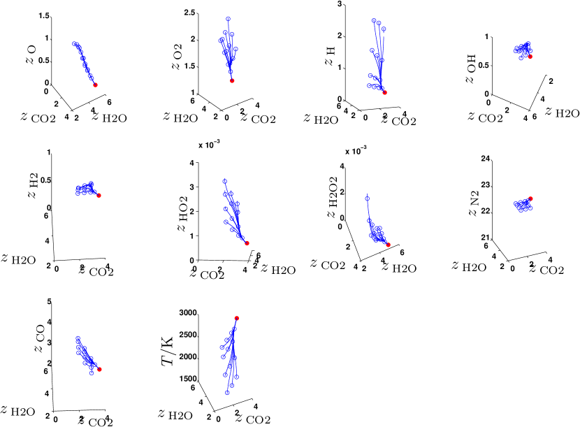
Figure 7: Visualization of the results (two-dimensional SIM) of the model reduction method applied to the syngas combustion model described in Section 5.3. The reverse mode is applied with a time horizon of ${10}^{-7}\text{\,}\mathrm{s}$. We approximate a two-dimensional manifold and use the overall products $z_{\mathrm{H}_{2}\mathrm{O}}$ and $z_{\mathrm{CO}_{2}}$ as reaction progress variables.

The same style as in Figure 3 is used. The resulting SIM approximation points (solutions of the optimization problem (10)) are shown as open blue dots together with trajectories emanating from these and converging to equilibrium, which is shown as full red dot. In the two-dimensional case, invariance cannot be seen by eye inspection, but a reasonable manifold is found.

6 Conclusions

An optimization method is presented that allows for efficient model reduction of realistic combustion models. It is applied to three models for testing its applicability. It can be seen that for an appropriate time scale separation the solution of an optimization problem approximates points on a slow invariant manifold. The application of the model reduction approach to a realistic syngas combustion model considered in an adiabatic and isochoric environment demonstrates the applicability to realistic large scale mechanisms.

Further research will be needed for an identification of an appropriate number and choice of the reaction progress variables for large scale mechanisms.

- (1) Al-Khateeb, A.N., Powers, J.M., Paolucci, S., Sommese, A.J., Diller, J.A., Hauenstein, J.D., Mengers, J.D.: One-dimensional slow invariant manifolds for spatially homogenous reactive systems. J. Chem. Phys. 131(2), 024,118 (2009)
- (2) Al-Khateeb, A.N.S.: Fine scale phenomena in reacting systems: Identification and analysis for their reduction. Ph.D. thesis, University of Notre Dame, Notre Dame, Indiana, USA (2010)
- (3) Amestoy, P.R., Duff, I.S., Koster, J., L’Excellent, J.Y.: A fully asynchronous multifrontal solver using distributed dynamic scheduling. SIAM J. Matrix. Anal. A. 23(1), 15–41 (2001)
- (4) Ascher, U., Petzold, L.: Computer methods for ordinary differential equations and differential-algebraic equations. SIAM, Philadelphia (1998)
- (5) Bell, B.M.: Automatic differentiation software cppad. (2010). URL http://www.coin-or.org/CppAD/
- (6) Bell, B.M., Burke, J.V.: Algorithmic differentiation of implicit functions and optimal values. In: C.H. Bischof, H.M. Bücker, P.D. Hovland, U. Naumann, J. Utke (eds.) Advances in Automatic Differentiation, pp. 67–77. Springer (2008)
- (7) Burcat, A., Ruscic, B.: Third millennium ideal gas and condensed phase thermochemical database for combustion with updates from active thermochemical tables. Tech. rep., Argonne National Laboratory (2005)
- (8) Curtiss, C.F., Hirschfelder, J.O.: Integration of stiff equations. Proc. Natl. Acad. Sci. USA 38, 235–243 (1952)
- (9) Davis, M.J., Skodje, R.T.: Geometric investigation of low-dimensional manifolds in systems approaching equilibrium. J. Chem. Phys. 111, 859–874 (1999)
- (10) Delhaye, S., Somers, L.M.T., van Oijen, J.A., de Goey, L.P.H.: Incorporating unsteady flow-effects in flamelet-generated manifolds. Combust. Flame 155(1-2), 133–144 (2008)
- (11) Forsgren, A., Gill, P.E., Wright, M.H.: Interior methods for nonlinear optimization. SIAM Rev. 44(4), 525–597 (2002)
- (12) Gilbert, R., Luther, K., Troe, J.: Theory of thermal unimolecular reactions in the fall-off range. ii. weak collision rate constants. Ber. Bunsenges. Phys. Chem. 87, 169–177 (1983)
- (13) Girimaji, S.S.: Reduction of large dynamical systems by minimization of evolution rate. Phys. Rev. Lett. 82(11), 2282–2285 (1999)
- (14) Gorban, A.N., Karlin, I.V.: Invariant Manifolds for Physical and Chemical Kinetics, Lecture Notes in Physics, vol. 660. Springer-Verlag Berlin Heidelberg New York (2005)
- (15) HSL: A collection of fortran codes for large-scale scientific computation. (2007). URL http://www.hsl.rl.ac.uk
- (16) Kee, R.J., Coltrin, M.E., Glarborg, P.: Chemically Reacting Flow: Theory and Practice. Wiley-Interscience, Hoboken, NJ (2003)
- (17) Ketelheun, A., Olbricht, C., Hahn, F., Janicka, J.: NO prediction in turbulent flames using LES/FGM with additional transport equations. Proc. Combust. Inst. 33(2), 2975–2982 (2011)
- (18) Lam, S.: Recent Advances in the Aerospace Sciences, chap. Singular Perturbation for Stiff Equations using Numerical Methods, pp. 3–20. Plenum Press, New York and London (1985)
- (19) Lam, S.H., Goussis, D.A.: The CSP method for simplifying kinetics. Int. J. Chem. Kinet. 26, 461–486 (1994)
- (20) Lebiedz, D.: Computing minimal entropy production trajectories: An approach to model reduction in chemical kinetics. J. Chem. Phys. 120(15), 6890–6897 (2004)
- (21) Lebiedz, D.: Entropy-related extremum principles for model reduction of dynamical systems. Entropy 12(4), 706–719 (2010)
- (22) Lebiedz, D., Reinhardt, V., Siehr, J.: Minimal curvature trajectories: Riemannian geometry concepts for slow manifold computation in chemical kinetics. J. Comput. Phys. 229(18), 6512–6533 (2010)
- (23) Lebiedz, D., Reinhardt, V., Siehr, J., Unger, J.: Geometric criteria for model reduction in chemical kinetics via optimization of trajectories. In: A.N. Gorban, D. Roose (eds.) Coping with Complexity: Model Reduction and Data Analysis, no. 75 in Lecture Notes in Computational Science and Engineering, first edn., pp. 241–252. Springer (2011)
- (24) Lebiedz, D., Siehr, J.: A continuation method for the efficient solution of parametric optimization problems in kinetic model reduction. arXiv:1301.5815 (2013). URL http://arxiv.org/abs/1301.5815
- (25) Lebiedz, D., Siehr, J., Unger, J.: A variational principle for computing slow invariant manifolds in dissipative dynamical systems. SIAM J. Sci. Comput. 33(2), 703–720 (2011)
- (26) Lee, J.M.: Introduction to Topological Manifolds, second edn. No. 202 in Graduate Texts in Mathematics. Springer, New York (2011)
- (27) Li, J., Zhao, Z., Kazakov, A., Dryer, F.L.: An updated comprehensive kinetic model of hydrogen combustion. Int. J. Chem. Kinet. 36(10), 566–575 (2004)
- (28) Maas, U., Pope, S.B.: Simplifying chemical kinetics: Intrinsic low-dimensional manifolds in composition space. Combust. Flame 88, 239–264 (1992)
- (29) Maas, U., Warnatz, J.: Simulation of thermal ignition processes in two-dimensional geometries. Z. Phys. Chem. N. F. 161, 61–81 (1989)
- (30) Najm, H.N., Valorani, M., Goussis, D.A., Prager, J.: Analysis of methane-air edge flame structure. Combust. Theor. Model. 14(2), 257–294 (2010)
- (31) Nocedal, J., Wright, S.J.: Numerical Optimization, second edn. Springer Series in Operations Research and Financial Engineering. Springer, New York (2006)
- (32) Powell, M.J.D.: A fast algorithm for nonlinearly constrained optimization calculations. In: A. Dold, B. Eckmann (eds.) Numerical Analysis, Lecture Notes in Mathematics, vol. 630, pp. 144–157. Springer-Verlag Berlin (1978)
- (33) Reinhardt, V., Winckler, M., Lebiedz, D.: Approximation of slow attracting manifolds in chemical kinetics by trajectory-based optimization approaches. J. Phys. Chem. A 112(8), 1712–1718 (2008)
- (34) Ren, Z., Pope, S.B., Vladimirsky, A., Guckenheimer, J.M.: The invariant constrained equilibrium edge preimage curve method for the dimension reduction of chemical kinetics. J. Chem. Phys. 124, 114,111 (2006)
- (35) Skanda, D.: Robust optimal experimental design for model discrimination of kinetic ODE systems. Ph.D. thesis, University of Freiburg, Freiburg im Breisgau, Germany (2012). URL http://www.freidok.uni-freiburg.de/volltexte/8787/
- (36) Smith, G.P., Golden, D.M., Frenklach, M., Moriarty, N.W., Eiteneer, B., Goldenberg, M., Bowman, C.T., Hanson, R.K., Song, S., Gardiner Jr., W.C., Lissianski, V.V., Qin, Z.: GRI-Mech 3.0. published online (1999). URL http://www.me.berkeley.edu/gri_mech
- (37) Troe, J.: Theory of thermal unimolecular reactions in the fall-off range. i. strong collision rate constants. Ber. Bunsenges. Phys. Chem. 87, 161–169 (1983)
- (38) Wächter, A., Biegler, L.T.: On the implementation of a primal-dual interior point filter line search algorithm for large-scale nonlinear programming. Math. Program. 106(1), 25–57 (2006)
- (39) Warnatz, J., Maas, U., Dibble, R.W.: Combustion: Physical and Chemical Fundamentals, Modeling and Simulation, Experiments, Pollutant Formation, fourth edn. Springer, Berlin (2006)
- (40) Wiggins, S.: Introduction to Applied Nonlinear Dynamical Systems and Chaos, third edn. No. 2 in Texts in Applied Mathematics. Springer, New York (1996)