Seesaw mechanism with four texture zeros
in the neutrino Yukawa matrix

Abstract

With the recent observation of nonzero $\theta_{13}$, five neutrino oscillation parameters are now known. By imposing four zeros in the Yukawa coupling matrix of the type I seesaw model, the number of parameters in the neutrino mass matrix is reduced to seven, and we are able to make predictions for the lightest neutrino mass, Dirac CP phase, and neutrinoless double beta decay. Four texture zeros in the Yukawa coupling matrix is equivalent to either a single texture zero or a single cofactor zero for an off-diagonal element of the light neutrino mass matrix. We find strong similarities between single texture zero models with one mass ordering and single cofactor zero models with the opposite mass ordering. In the context of a specific class of single-flavor leptogenesis models, we find additional constraints on the parameter space.

1 Introduction

Low-energy neutrino phenomenology is described by nine parameters in the Majorana mass matrix of light neutrinos, which can be written as [1] $M=V^{*}\text{diag}(m_{1},m_{2},m_{3})V^{\dagger}$, with $V=U\text{diag}(1,e^{i\phi_{2}/2},e^{i\phi_{3}/2})$ and

$$U=\begin{bmatrix}c_{13}c_{12}&c_{13}s_{12}&s_{13}e^{-i\delta}\\ -s_{12}c_{23}-c_{12}s_{23}s_{13}e^{i\delta}&c_{12}c_{23}-s_{12}s_{23}s_{13}e^{i\delta}&s_{23}c_{13}\\ s_{12}s_{23}-c_{12}c_{23}s_{13}e^{i\delta}&-c_{12}s_{23}-s_{12}c_{23}s_{13}e^{i\delta}&c_{23}c_{13}\end{bmatrix}.$$ (1)

After the measurement of $\theta_{13}$ by the Daya Bay [2], RENO [3], and Double Chooz [4] experiments, five of them are known; the result of a recent global three-neutrino fit [5] is shown in Table 1. The tiny masses of light neutrinos can be elegantly explained by the seesaw mechanism [6], but, unfortunately, with the introduction of additional free parameters that cannot be measured in the forseeable future. The most popular seesaw model is the type I seesaw, in which the mass matrix of the light neutrinos can be written as

$$M=\lambda^{T}{M_{R}}^{-1}\lambda v^{2}=Y^{T}Y\,,$$ (2)

where, for $N$ heavy right-handed neutrinos, ${M_{R}}=\text{diag}(M_{1},M_{2},\cdots,M_{N})$, $\lambda$ is a $N\times 3$ Yukawa coupling matrix, and

$$Y=v{M_{R}}^{-1/2}\lambda=\begin{bmatrix}y_{1e}&y_{1\mu}&y_{1\tau}\\ y_{2e}&y_{2\mu}&y_{2\tau}\\ \vdots&\vdots&\vdots\\ y_{Ne}&y_{N\mu}&y_{N\tau}\end{bmatrix}.$$ (3)

Note that on permuting the rows of the Y matrix (which is equivalent to reordering the right-handed neutrinos) or applying a rotation to the rows of the $Y$ matrix (which is equivalent to a rotation in the space of the right-handed neutrinos), the mass matrix of the light neutrinos remains the same.

The standard seesaw model has $N=3$ and permits any set of low-energy neutrino parameters in $M_{\nu}$. A way to extract predictions from the seesaw model is to impose constraints on its parameters. The most economical seesaw model includes two right-handed neutrinos and two zeros in the Yukawa coupling matrix, or, equivalently, two zeros in $Y$ [7]. The measurement of $\theta_{13}$ excludes the normal mass ordering (NO) and stringently constrains the allowed parameter space for the inverted mass ordering (IO); in particular, the phase $\delta$ must be such that Dirac CP violation is close to maximal [8]. Also, for two right-handed neutrinos, one of the light neutrinos must have vanishing mass, so the allowed values of the sum of all light neutrino masses (which affects structure formation in our universe) and $|M_{ee}|$ (which determines the rate for neutrinoless double-beta decay ($0\nu\beta\beta$), a signal of lepton number violation) are limited.

Table 1: Best-fit values and $2\sigma$ ranges of the oscillation parameters [5], with $\delta m^{2}\equiv m_{2}^{2}-m_{1}^{2}$ and $\Delta m^{2}\equiv m_{3}^{2}-(m_{1}^{2}+m_{2}^{2})/2$.

Ordering	$\theta_{12}(^{\circ})$	$\theta_{13}(^{\circ})$	$\theta_{23}(^{\circ})$	$\delta m^{2}(10^{-5}\text{eV}^{2})$	$|\Delta m^{2}|(10^{-3}\text{eV}^{2})$
Normal	$33.6^{+2.1}_{-2.0}$	$8.9^{+0.9}_{-0.9}$	$38.4^{+3.6}_{-2.3}$	$7.54^{+0.46}_{-0.39}$	$2.43^{+0.12}_{-0.16}$
Inverted	$33.6^{+2.1}_{-2.0}$	$9.0^{+0.8}_{-1.0}$	$38.8^{+5.3}_{-2.3}\oplus 47.5-53.2$	$7.54^{+0.46}_{-0.39}$	$2.42^{+0.11}_{-0.16}$

In this paper, we extend this most economical model to include a third right-handed neutrino. We use texture zeros in $Y$ as extra constraints, which may arise in, e.g., extra dimensional models [8]. If there are 5 or more texture zeros in $Y$, the most economical model with two right-handed neutrinos or a block diagonal matrix is obtained; the latter is excluded by the current experimental data. So the simplest case for three right-handed neutrinos has four texture zeros in $Y$, which is equivalent to five nonzero elements; for previous work see Refs. [9, 10]. Here we derive analytic formulas that relate the free parameters to the dependent ones and determine the constraints on these models including the recent data on $\theta_{13}$.

With five nonzero elements in $Y$ only two phases are physical, so that there are seven free parameters in the four texture zero model. Hence, we can use the five observed oscillation parameters from the global fit to determine the allowed regions for the Dirac CP phase $\delta$ and $m_{1}$ ($m_{3}$) for the normal (inverted) ordering. Then we can obtain the values of the Majorana phases $\phi_{2}$ and $\phi_{3}$, completing our knowledge of all the elements in the light neutrino mass matrix. Furthermore, from Eq. (2) we can find $Y$ and then study neutrinoless double beta decay and leptogenesis.

In Sec. 2, we list the general properties of the four texture zero model and give a brief review of neutrinoless double beta decay and leptogenesis. In Sec. 3, we use current experimental data to study the allowed parameter regions for each texture. We conclude in Sec. 4.

2 Classes with four texture zeros

There are 3 basic ways to have 5 nonzero elements: (2, 2, 1), (3, 1, 1) or (3, 2, 0), where the numbers indicate how many nonzero elements are in each row of the $Y$ matrix. The (3, 2, 0) case is equivalent to two right-handed neutrinos with one texture zero element and one vanishing mass, and is equivalent to the most economical $N=2$ model after a rotation in the right-handed neutrino space. So only the (2, 2, 1) and (3, 1, 1) cases need to be considered. There are 9 independent textures in the (2, 2, 1) case and 3 independent textures in the (3, 1, 1) case. We divide them into four classes:

Class 1

$$1A:\begin{bmatrix}\times&\times&0\\ \times&0&\times\\ \times&0&0\end{bmatrix}\quad 1B:\begin{bmatrix}\times&\times&0\\ \times&0&\times\\ 0&\times&0\end{bmatrix}\quad 1C:\begin{bmatrix}\times&\times&0\\ \times&0&\times\\ 0&0&\times\end{bmatrix}$$

Class 2

$$2A:\begin{bmatrix}\times&\times&0\\ 0&\times&\times\\ \times&0&0\end{bmatrix}\quad 2B:\begin{bmatrix}\times&\times&0\\ 0&\times&\times\\ 0&\times&0\end{bmatrix}\quad 2C:\begin{bmatrix}\times&\times&0\\ 0&\times&\times\\ 0&0&\times\end{bmatrix}$$

Class 3

$$3A:\begin{bmatrix}\times&0&\times\\ 0&\times&\times\\ \times&0&0\end{bmatrix}\quad 3B:\begin{bmatrix}\times&0&\times\\ 0&\times&\times\\ 0&\times&0\end{bmatrix}\quad 3C:\begin{bmatrix}\times&0&\times\\ 0&\times&\times\\ 0&0&\times\end{bmatrix}$$

Class 4

$$4A:\begin{bmatrix}\times&\times&\times\\ 0&\times&0\\ 0&0&\times\end{bmatrix}\quad 4B:\begin{bmatrix}\times&\times&\times\\ 0&0&\times\\ \times&0&0\end{bmatrix}\quad 4C:\begin{bmatrix}\times&\times&\times\\ \times&0&0\\ 0&\times&0\end{bmatrix}$$

For each class there are six possible permutations of the rows, so there are 72 individual cases in all [9].

The rate for neutrinoless double beta decay depends on the effective Majorana mass, which is equal to the magnitude of the $\nu_{e}-\nu_{e}$ element of the neutrino mass matrix,

$$|M_{ee}|=|m_{1}c_{12}^{2}c_{13}^{2}+m_{2}e^{-i\phi_{2}}s_{12}^{2}c_{13}^{2}+m_{3}e^{-i\phi_{3}}s_{13}^{2}e^{2i\delta}|.$$ (4)

Note that $|M_{ee}|$ can be written in a form that is independent of the Dirac CP phase $\delta$ by redefining $\phi_{3}$. We choose the form above because the Majorana phases will be constrained. The latest experimental result from EXO-200 [11] shows that the effective mass is less than $140-380$ meV at 90% C.L. In the foreseeable future, experiments such as KamLAND-Zen will reach a sensitivity of about 50 meV or below [12].

In principle, leptogenesis may provide hints of the structure of the Yukawa matrix; see Ref. [13] for a recent review. In what follows, we adopt a minimal scenario of leptogenesis [14]. We work in the single flavor approximation in which $M_{1}>10^{12}$ GeV, so that the flavor composition of the leptons does not affect the baryon asymmetry of the universe. We also assume the right-handed neutrinos to be hierarchical, $M_{2},M_{3}\gg M_{1}>10^{12}$ GeV. Then in the standard model the baryon asymmetry is given by [14]

$$\eta_{B0}=\frac{n_{B}}{n_{\gamma}}=-9.72\times 10^{-3}\times\epsilon_{1}\times\eta,$$ (5)

where $\epsilon_{1}$ is the CP asymmetry in the decay of the lightest right-handed neutrino, and $\eta$ is the wash out efficiency factor, which can be obtained by solving the Boltzmann equation. We use a very simple analytic fit [14]

$$\eta\simeq\left(\frac{0.55\times 10^{-3}\text{ eV}}{\tilde{m}_{1}}\right)^{1.16},$$ (6)

where $\tilde{m}_{1}$ is

$$\tilde{m}_{1}=\sum_{\begin{subarray}{c}\alpha=e,\mu,\tau\end{subarray}}|\lambda_{1\alpha}|^{2}\frac{v^{2}}{M_{1}}=\sum_{\begin{subarray}{c}\alpha=e,\mu,\tau\end{subarray}}|y_{1\alpha}|^{2}.$$ (7)

Equation (6) is valid for $M_{1}\ll 10^{14}$ GeV and $\tilde{m}_{1}\geq 0.01$ eV. With these constraints, the baryon asymmetry is

$$\eta_{B0}=\frac{n_{B}}{n_{\gamma}}\simeq-3.4\times 10^{-4}\times\epsilon_{1}(\frac{0.01\text{eV}}{\tilde{m}_{1}})^{1.16},$$ (8)

where $\epsilon_{1}$ can be written as

$$\epsilon_{1} =-\frac{3}{16\pi}\frac{M_{1}}{(\lambda\lambda^{\dagger})_{11}}\text{Im}[(\lambda\lambda^{\dagger}M_{R}^{-1}(\lambda\lambda^{\dagger})^{T})_{11}]$$

$$=-\frac{3}{16\pi}\frac{1}{(\lambda\lambda^{\dagger})_{11}}\sum_{\begin{subarray}{c}j\neq 1\end{subarray}}\text{Im}(\lambda\lambda^{\dagger})_{1j}^{2}\frac{M_{1}}{M_{j}}.$$ (9)

Since $\lambda=\frac{1}{v}M_{R}^{1/2}Y$, we have

$$\epsilon_{1} =-\frac{3}{16\pi}\frac{M_{1}}{v^{2}(YY^{\dagger})_{11}}\sum_{\begin{subarray}{c}j\neq 1\end{subarray}}\text{Im }(YY^{\dagger})_{1j}^{2}$$

$$=-\frac{3M_{1}}{16\pi v^{2}}\sum_{\begin{subarray}{c}j\neq 1\end{subarray}}\frac{\text{Im}(y_{1e}y_{je}^{*}+y_{1\mu}y_{j\mu}^{*}+y_{1\tau}y_{j\tau}^{*})^{2}}{|y_{1e}|^{2}+|y_{1\mu}|^{2}+|y_{1\tau}|^{2}}.$$ (10)

Hence, the baryon asymmetry is proportional to the lightest right handed neutrino mass $M_{1}$. The observed baryon asymmetry is $\eta_{B0}=6.19\times 10^{-10}$ [15]. Since $Y$ is determined by the light neutrino mass matrix, we can calculate the lightest right-handed neutrino mass $M_{1}$ from Eqs. (7), (8), and (10), ensuring that $10^{12}\text{ GeV}<M_{1}\ll 10^{14}$ GeV.

3 Phenomenology

3.1 Class 1 ($M_{23}=0$)

The mass matrices of the three textures in Class 1 always have a zero in the (2, 3) entry. In fact, $M_{23}=0$ is the only condition on $Y$ for all the textures in Class 1, and the condition is the same for both mass orderings (normal and inverted). Take Class 1A for example; we can write

$$Y=\begin{bmatrix}a&b&0\\ c&0&d\\ e&0&0\end{bmatrix}\,,$$ (11)

where $a,b,c,d,e$ are all nonzero complex numbers. Then the mass matrix of the light neutrinos becomes

$$M=Y^{T}Y=\begin{bmatrix}a^{2}+c^{2}+e^{2}&ab&cd\\ ab&b^{2}&0\\ cd&0&d^{2}\end{bmatrix}.$$ (12)

Comparing Eq. (12) with the standard parametrization, if $M_{23}=0$, we can find a solution for $Y$ as follows:

$$b=\pm M_{22}^{1/2},a=M_{12}/b,d=\pm M_{33}^{1/2},c=M_{13}/d,e=\pm(M_{11}-a^{2}-c^{2})^{1/2}.$$ (13)

Since $a,b,c,d,e$ are all nonzero complex numbers, a solution always exists. Solutions for $Y$ for the other two textures in Class 1 may be derived in a similar fashion. Therefore, Class 1 is defined by the necessary and sufficient condition $M_{23}=0$, which can be written as

$$m_{1}=-{m_{3}e^{i\phi_{3}}U_{\tau 3}U_{\mu 3}+m_{2}e^{i\phi_{2}}U_{\tau 2}U_{\mu 2}\over U_{\tau 1}U_{\mu 1}}.$$ (14)

Taking the absolute square gives

$$m_{1}^{2}|U_{\mu 1}|^{2}|U_{\tau 1}|^{2}-m_{2}^{2}|U_{\mu 2}|^{2}|U_{\tau 2}|^{2}-m_{3}^{2}|U_{\mu 3}|^{2}|U_{\tau 3}|^{2}=2{\rm Re}(m_{3}e^{-i\phi_{3}}U_{\mu 3}^{*}U_{\tau 3}^{*}m_{2}e^{i\phi_{2}}U_{\mu 2}U_{\tau 2}),$$ (15)

or, defining $\phi=\phi_{3}-\phi_{2}$,

$$m_{1}^{2} |U_{\mu 1}|^{2}|U_{\tau 1}|^{2}-m_{2}^{2}|U_{\mu 2}|^{2}|U_{\tau 2}|^{2}-m_{3}^{2}|U_{\mu 3}|^{2}|U_{\tau 3}|^{2}$$ (16)

$$= -2m_{2}m_{3}c_{13}^{2}s_{23}c_{23}{\rm Re}\left[e^{-i\phi}(c_{12}c_{23}-s_{12}s_{23}s_{13}e^{i\delta})(c_{12}s_{23}+s_{12}c_{23}s_{13}e^{i\delta})\right]$$

$$= -2m_{2}m_{3}c_{13}^{2}s_{23}c_{23}\times$$

$${\rm Re}\left[c_{12}^{2}s_{23}c_{23}\cos\phi+s_{12}c_{12}s_{13}(c_{23}^{2}-s_{23}^{2})\cos(\phi-\delta)-s_{12}^{2}s_{23}c_{23}s_{13}^{2}\cos(\phi-2\delta)\right].$$

Expanding the cosines yields the form

$$C=A\cos\phi+B\sin\phi,$$ (17)

with A, B and C as listed in Table 2.

$C=A\cos\phi+B\sin\phi$
Class A B C 1 $\begin{array}[]{l}-2m_{2}m_{3}c_{13}^{2}s_{23}c_{23}\times\\ \left[c_{12}^{2}s_{23}c_{23}+s_{12}c_{12}s_{13}(c_{23}^{2}-s_{23}^{2})\cos\delta\right.\\ \left.-s_{12}^{2}s_{23}c_{23}s_{13}^{2}\cos(2\delta)\right]\end{array}$ $\begin{array}[]{l}-2m_{2}m_{3}c_{13}^{2}s_{23}c_{23}s_{12}s_{13}\times\\ \left[c_{12}(c_{23}^{2}-s_{23}^{2})\sin\delta\right.\\ \left.-s_{12}s_{23}c_{23}s_{13}\sin(2\delta)\right]\end{array}$ $\begin{array}[]{l}m_{1}^{2}|U_{\mu 1}|^{2}|U_{\tau 1}|^{2}\\ -m_{2}^{2}|U_{\mu 2}|^{2}|U_{\tau 2}|^{2}\\ -m_{3}^{2}|U_{\mu 3}|^{2}|U_{\tau 3}|^{2}\end{array}$ 2 $\begin{array}[]{l}-2m_{2}m_{3}c_{13}^{2}s_{12}c_{23}s_{13}\times\\ \left[c_{12}s_{23}\cos\delta+s_{12}c_{23}s_{13}\cos(2\delta)\right]\end{array}$ $\begin{array}[]{l}-2m_{2}m_{3}c_{13}^{2}s_{12}c_{23}s_{13}\times\\ \left[c_{12}s_{23}\sin\delta+s_{12}c_{23}s_{13}\sin(2\delta)\right]\end{array}$ $\begin{array}[]{l}m_{1}^{2}|U_{e1}|^{2}|U_{\tau 1}|^{2}\\ -m_{2}^{2}|U_{e2}|^{2}|U_{\tau 2}|^{2}\\ -m_{3}^{2}|U_{e3}|^{2}|U_{\tau 3}|^{2}\end{array}$ 3 $\begin{array}[]{l}2m_{2}m_{3}c_{13}^{2}s_{12}s_{23}s_{13}\times\\ \left[c_{12}c_{23}\cos\delta-s_{12}s_{23}s_{13}\cos(2\delta)\right]\end{array}$ $\begin{array}[]{l}2m_{2}m_{3}c_{13}^{2}s_{12}s_{23}s_{13}\times\\ \left[c_{12}c_{23}\sin\delta-s_{12}s_{23}s_{13}\sin(2\delta)\right]\end{array}$ $\begin{array}[]{l}m_{1}^{2}|U_{e1}|^{2}|U_{\mu 1}|^{2}\\ -m_{2}^{2}|U_{e2}|^{2}|U_{\mu 2}|^{2}\\ -m_{3}^{2}|U_{e3}|^{2}|U_{\mu 3}|^{2}\end{array}$ 4A $\begin{array}[]{l}-2m_{2}^{-1}m_{3}^{-1}c_{13}^{2}s_{23}c_{23}\times\\ \left[c_{12}^{2}s_{23}c_{23}+s_{12}c_{12}s_{13}(c_{23}^{2}-s_{23}^{2})\cos\delta\right.\\ \left.-s_{12}^{2}s_{23}c_{23}s_{13}^{2}\cos(2\delta)\right]\end{array}$ $\begin{array}[]{l}-2m_{2}^{-1}m_{3}^{-1}c_{13}^{2}s_{23}c_{23}s_{12}s_{13}\times\\ \left[c_{12}(c_{23}^{2}-s_{23}^{2})\sin\delta\right.\\ \left.-s_{12}s_{23}c_{23}s_{13}\sin(2\delta)\right]\end{array}$ $\begin{array}[]{l}m_{1}^{-2}|U_{\mu 1}|^{2}|U_{\tau 1}|^{2}\\ -m_{2}^{-2}|U_{\mu 2}|^{2}|U_{\tau 2}|^{2}\\ -m_{3}^{-2}|U_{\mu 3}|^{2}|U_{\tau 3}|^{2}\end{array}$ 4B $\begin{array}[]{l}-2m_{2}^{-1}m_{3}^{-1}c_{13}^{2}s_{12}c_{23}s_{13}\times\\ \left[c_{12}s_{23}\cos\delta+s_{12}c_{23}s_{13}\cos(2\delta)\right]\end{array}$ $\begin{array}[]{l}-2m_{2}^{-1}m_{3}^{-1}c_{13}^{2}s_{12}c_{23}s_{13}\times\\ \left[c_{12}s_{23}\sin\delta+s_{12}c_{23}s_{13}\sin(2\delta)\right]\end{array}$ $\begin{array}[]{l}m_{1}^{-2}|U_{e1}|^{2}|U_{\tau 1}|^{2}\\ -m_{2}^{-2}|U_{e2}|^{2}|U_{\tau 2}|^{2}\\ -m_{3}^{-2}|U_{e3}|^{2}|U_{\tau 3}|^{2}\end{array}$ 4C $\begin{array}[]{l}2m_{2}^{-1}m_{3}^{-1}c_{13}^{2}s_{12}c_{23}s_{13}\times\\ \left[c_{12}c_{23}\cos\delta-s_{12}s_{23}s_{13}\cos(2\delta)\right]\end{array}$ $\begin{array}[]{l}2m_{2}^{-1}m_{3}^{-1}c_{13}^{2}s_{12}c_{23}s_{13}\times\\ \left[c_{12}c_{23}\sin\delta-s_{12}s_{23}s_{13}\sin(2\delta)\right]\end{array}$ $\begin{array}[]{l}m_{1}^{-2}|U_{e1}|^{2}|U_{\mu 1}|^{2}\\ -m_{2}^{-2}|U_{e2}|^{2}|U_{\mu 2}|^{2}\\ -m_{3}^{-2}|U_{e3}|^{2}|U_{\mu 3}|^{2}\end{array}$

Table 2: The coefficients A, B and C for each class.

For Eq. (17), if $C^{2}>A^{2}+B^{2}$, there is no solution; if $C^{2}<A^{2}+B^{2}$, there are two solutions:

$$\phi=2\arctan\frac{B\pm\sqrt{A^{2}+B^{2}-C^{2}}}{A+C}.$$ (18)

We can write Eq. (14) in terms of $\phi$ as

$$m_{1}=e^{i\phi_{2}}\frac{-m_{3}e^{i\phi}U_{\tau 3}U_{\mu 3}-m_{2}U_{\tau 2}U_{\mu 2}}{U_{\tau 1}U_{\mu 1}}.$$ (19)

Since $m_{1}$ is a non-negative real number, we get

$$\phi_{2}=-\text{arg}[\frac{-m_{3}e^{i\phi}U_{\tau 3}U_{\mu 3}-m_{2}U_{\tau 2}U_{\mu 2}}{U_{\tau 1}U_{\mu 1}}],$$ (20)

and

$$\phi_{3}=\phi_{2}+\phi.$$ (21)

Therefore, if $m_{1}$ ($m_{3}$) and $\delta$ in the normal (inverted) ordering are known, we can calculate A, B and C using the five measured oscillation parameters in Table 1. We scan the $\delta$ and $m_{1}$ ($m_{3}$) space to find the allowed regions, which are defined by the condition $C^{2}<A^{2}+B^{2}$ (see Fig. 1 for the normal ordering and the upper panel of Fig. 2 for the inverted ordering). We show allowed regions corresponding to the best-fit parameters, and those allowed at $2\sigma$. We also plot iso-$\phi_{2}$ and iso-$|M_{ee}|$ contours using the best-fit oscillation parameters. We only show the contours for the plus sign of $\phi$ in Eq. (18) because changing $\delta$ to $360^{\circ}-\delta$ yields the same contours for the minus solution.

The allowed regions can be further constrained using leptogenesis. We assume the lightest right-handed neutrino has mass between $10^{12}$ GeV and $10^{13}$ GeV and is much lighter than the others so that we can use Eq. (8). We also require $\tilde{m}_{1}\geq 0.01$ eV. From Eqs. (7) and (10), we see that the baryon asymmetry depends on the sign choices of $\phi$ in Eq. (18) but not on the sign choices in Eq. (13), because different choices of signs in Eq. (13) change the signs of all parameters in one row of the $Y$ matrix, which yield the same baryon asymmetry. The baryon asymmetry also depends on the row of $Y$ that is associated with the lightest right-handed neutrino mass, but the order of the other two rows does not affect the baryon asymmetry.

Since Classes 1A, 1B and 1C have different textures, the allowed regions for successful leptogenesis are also different in these three cases. Here we only consider Class 1A as an example. We find that successful leptogenesis is not possible for the normal ordering. For the inverted ordering, the allowed regions are shown in the three lower panels of Fig. 2. Although the constraints on $\delta$ vary according to which right-handed neutrino is lightest, in no case is the lightest left-handed neutrino allowed to be above 100 meV.

3.2 Class 2 ($M_{13}=0$)

Similar to Class 1, the only condition for Class 2 is $M_{13}=0$, which is independent of ordering and can be written as

$$m_{1}=-{m_{3}e^{i\phi_{3}}U_{\tau 3}U_{e3}+m_{2}e^{i\phi_{2}}U_{\tau 2}U_{e2}\over U_{\tau 1}U_{e1}}.$$ (22)

After taking the absolute square, then as in Class 1 this may be put in the form of Eq. (17), with A, B and C as in Table 2.

The solutions for $\phi_{2}$ and $\phi_{3}$ then proceed as in Class 1. The allowed regions for the inverted ordering are shown in Fig. 3, along with iso-$\phi_{2}$ and iso-$|M_{ee}|$ contours. We see that the solution found in Ref. [8] with $\lambda_{1e}=\lambda_{2\tau}=0$ or $\lambda_{1\tau}=\lambda_{2e}=0$ for the inverted ordering is a special case of our model with $m_{3}=0$. Leptogenesis predictions for Class 2A IO are also shown in Fig. 3, and give an upper bound on $m_{3}$ of about 200 meV. The allowed regions for the normal ordering are similar to Fig. 4.

3.3 Class 3 ($M_{12}=0$)

The only condition for Class 3 is $M_{12}=0$, which can be written

$$m_{1}=-{m_{3}e^{i\phi_{3}}U_{\mu 3}U_{e3}+m_{2}e^{i\phi_{2}}U_{\mu 2}U_{e2}\over U_{\mu 1}U_{e1}}.$$ (23)

This condition is the same for both mass orderings and as before this may be put in the form of Eq. (17) with A, B and C as in Table 2.

Note that Class 3 is the same as Class 2 for any ordering with $U_{\tau j}\to U_{\mu j}$, or $s_{23}\to-c_{23}$ and $c_{23}\to s_{23}$, which is the same as $\delta\to\delta+180^{\circ}$ when $\theta_{23}=45^{\circ}$. Since $\theta_{23}\approx 45^{\circ}$, the phenomenology of Classes 2 and 3 will be similar. The allowed regions for the normal ordering are shown in Fig. 4; also shown are predictions for $|M_{ee}|$ and $\phi_{2}$ and regions compatible with leptogenesis. The allowed regions for the inverted ordering are similar to those for Class 2 in Fig. 3 with $\delta\to\delta+180^{\circ}$. We note that the solution found in Ref. [8] with $\lambda_{1e}=\lambda_{2\mu}=0$ or $\lambda_{1\mu}=\lambda_{2e}=0$ for the inverted ordering is a special case in our model with $m_{3}=0$.

3.4 Class 4A ($(M^{-1})_{23}=0$)

Class 4 has no texture zeros in the mass matrix. However, the existence of a solution for $Y$ still depends on only one condition. Take Class 4A for example, in which case

$$Y=\begin{bmatrix}a&b&c\\ 0&d&0\\ 0&0&e\end{bmatrix}\,,$$ (24)

where $a,b,c,d,e$ are all nonzero complex numbers. Then the mass matrix becomes

$$M=Y^{T}Y=\begin{bmatrix}a^{2}&ab&ac\\ ab&b^{2}+d^{2}&bc\\ ac&bc&c^{2}+e^{2}\end{bmatrix},$$ (25)

and we see that if $\frac{M_{11}}{M_{12}}=\frac{M_{13}}{M_{23}}$ is satisfied, the other variables can be directly determined. Hence the Class 4A condition is equivalent to $M_{11}M_{23}=M_{12}M_{13}$, which means the (2, 3) cofactor of $M$, $C_{23}=M_{12}M_{31}-M_{11}M_{32}$, vanishes. Since $(M^{-1})_{ij}=\frac{1}{\det M}C_{ji}$, the condition for Class 4A is equivalent to $(M^{-1})_{23}=0$, i.e., a texture zero in the inverse mass matrix. Since $M^{-1}=V\text{diag}(m_{1}^{-1},m_{2}^{-1},m_{3}^{-1})V^{T}$, we can write the condition as

$$m_{1}^{-1}U_{\tau 1}U_{\mu 1}+m_{2}^{-1}e^{i\phi_{2}}U_{\tau 2}U_{\mu 2}+m_{3}^{-1}e^{i\phi_{3}}U_{\tau 3}U_{\mu 3}=0\,,$$ (26)

or

$$m_{1}^{-1}=-\frac{m_{2}^{-1}e^{i\phi_{2}}U_{\tau 2}U_{\mu 2}+m_{3}^{-1}e^{i\phi_{3}}U_{\tau 3}U_{\mu 3}}{U_{\tau 1}U_{\mu 1}}.$$ (27)

The allowed regions for the normal ordering are shown in Fig. 5. The allowed regions for the inverted ordering are similar to Fig. 1 (Class 1 NO), and the iso-$\phi_{2}$ and iso-$|M_{ee}|$ contours are similar with $\phi_{2}\to-\phi_{2}$. The similarity of an IO scenario with an NO one may seem unusual, but can be understood by looking at the form of the $A$, $B$, and $C$ coefficients in Table 2; multiplying the coefficients for Class 4A IO by $m_{2}m_{3}$, and dividing the coefficients for Class 1 NO by $m_{2}m_{3}$, we see that $A$ and $B$ are the same for the two cases. For the $C$ coefficient, the dominant term in each case is the third one, proportional to $|U_{\mu 3}|^{2}|U_{\tau 3}|^{2}$ times the ratio of a larger mass to a smaller one.

The comparison of Class 4A NO with Class 1 IO is more nuanced: when the lightest mass ($m_{1}$ for NO, $m_{3}$ for IO) is very small, the first two terms in the $C$ coefficient have similar size for Class 1 IO, but only the first term is dominant for Class 4A NO. However, when the lightest mass is not so small, such that $m_{1}\approx m_{2}$ in the NO, then the same terms in the $C$ coefficient are dominant. Thus for higher values of the lightest mass, although not necessarily so large that all three masses are quasi-degenerate, Classes 4A NO and 1 IO give similar predictions. This can be seen by comparing Figs. 5 and 2: although the allowed regions and contours are quite different when the lightest mass is below 20 meV, note the similarity of the $|M_{ee}|=100$ meV and $\phi_{2}=60^{\circ}$ contours.

3.5 Class 4B ($(M^{-1})_{13}=0$)

Similar to Class 4A, the condition for Class 4B is $(M^{-1})_{13}=0$, which can be written as

$$m_{1}^{-1}=-\frac{m_{2}^{-1}e^{i\phi_{2}}U_{\tau 2}U_{e2}+m_{3}^{-1}e^{i\phi_{3}}U_{\tau 3}U_{e3}}{U_{\tau 1}U_{e1}}.$$ (28)

This condition is the same for both mass orderings, and the analysis follows as in previous classes, with A, B and C given in Table 2.

The allowed regions for the normal (inverted) ordering are shown in Fig. 6 (Fig. 7). The inverted ordering for this case is also similar to Class 2 NO: multiplying the $A$, $B$, and $C$ coefficients by $m_{2}m_{3}$ for Class 4B IO and dividing them by $m_{2}m_{3}$ for Class 2 NO, $A$ and $B$ are identical for the two cases, and the dominant terms in $C$ are also the same. As was true in the previous section, the reverse correspondence between Class 4B NO and Class 2 IO exists only for larger values of the lightest mass (see Figs. 6 and 3 when the lightest mass is above 50 meV).

3.6 Class 4C ($(M^{-1})_{12}=0$)

Similar to Class 4A, the condition for Class 4C is $(M^{-1})_{12}=0$, which can be written as

$$m_{1}^{-1}=-\frac{m_{2}^{-1}e^{i\phi_{2}}U_{\mu 2}U_{e2}+m_{3}^{-1}e^{i\phi_{3}}U_{\mu 3}U_{e3}}{U_{\mu 1}U_{e1}}.$$ (29)

The corresponding values of A, B and C in Eq. (17) are given in Table 2.

Note that Class 4C is the same as Class 4B with $U_{\tau j}\to U_{\mu j}$, or $s_{23}\to-c_{23}$ and $c_{23}\to s_{23}$. As noted in Sec. 3.3, this transformation is equivalent to $\delta\to\delta+180^{\circ}$ when $\theta_{23}=45^{\circ}$. Therefore the allowed regions of Class 4C are similar to Class 4B in Fig. 6 for the normal ordering and in Fig. 7 for the inverted ordering with $\delta\to\delta+180^{\circ}$.

The inverted ordering for this case is also similar to Class 3 NO, as can be seen by examining the $A$, $B$ and $C$ coefficients, and Class 4C NO and Class 3 IO give similar results for larger values of the lightest mass. Thus there is a general pattern that the texture zero NO and corresponding cofactor zero IO have similar predictions, and texture zero IO and corresponding cofactor zero NO have similar predictions when the lightest mass is not too small.

4 Conclusions

We extended the most economical type I seesaw model to include three right-handed neutrinos. The simplest cases that fit the data have four texture zeros in the Yukawa couplings that connect the left-handed and right-handed neutrinos. These are equivalent to a single texture or cofactor zero for an off-diagonal element of the light neutrino mass matrix $M$. The cofactor zero condition is itself equivalent to a texture zero in $M^{-1}$. We used the latest experimental data to obtain the allowed regions for the lightest neutrino mass and Dirac CP phase $\delta$, which can be measured in future neutrino experiments. We also used leptogenesis to further constrain the allowed regions; in general there is an upper bound on the lightest neutrino mass of about 100-200 meV for a single-flavored leptogenesis scenario. Figures 2 to 7 show that in any given model, not all values of $\delta$ are consistent with the leptogenesis predictions. Therefore a precise measurement of $\delta$ will reduce the number of viable models.

Once the lightest neutrino mass and Dirac CP phase are determined, these models make definite predictions for neutrinoless double beta decay. From the iso-$|M_{ee}|$ contours in Figs. 1-7 we see that $|M_{ee}|$ is generally proportional to the lightest mass. This behavior is clearly evident for the quasi-degenerate spectrum. However, for some classes, $|M_{ee}|$ is strongly dependent on the Dirac CP phase $\delta$ and is not determined by the lightest mass alone. We plot the allowed regions in the $(|M_{ee}|,\rm{lightest\ mass})$ plane for these classes separately; see Figs. 8, 9, 10 and 11.

Table 3: The minimum values of $|M_{ee}|$ (in $10^{-3}$ eV) in each class for the best-fit oscillation parameters, and the $2\sigma$ lower bounds.

Class	Best-fit		$2\sigma$ lower bound
	NO	IO	NO	IO
1	142.5	19.0	129.8	15.4
2	1.4	46.9	0.3	44.8
3	0.0	47.4	0.0	45.2
4A	0.0	150.3	0.0	138.3
4B	6.1	18.4	5.7	15.1
4C	8.4	18.2	7.5	14.9

The minimum value of $|M_{ee}|$ for the best-fit oscillation parameters and the $2\sigma$ lower bounds are shown in Table 3. We find that the Class 1 NO and Class 4A IO have a minimum value for $|M_{ee}|$ of around 150 (130) meV for the best-fit parameters (at 2$\sigma$), and could therefore be excluded by the $0\nu\beta\beta$ decay experiments that are currently running; Classes 2 IO and 3 IO have a minimum $|M_{ee}|$ of around 50 meV and can be definitively tested by experiments under construction. For Classes 3 NO and 4A NO the current lower bound on $|M_{ee}|$ is zero, and given the current measurements of the oscillation parameters, $0\nu\beta\beta$ decay will not constrain them. The remaining models have a minimum $|M_{ee}|$ in the range $1-20$ meV and can only be completely probed by significant improvements in the sensitivity of $0\nu\beta\beta$ experiments. The sum of light neutrino masses can also be used to provide additional discrimination among these models. However, there is a general pattern that a texture zero NO and the corresponding cofactor zero IO have similar predictions, and a texture zero IO and the corresponding cofactor zero NO have similar predictions when the lightest mass is not too small. Therefore it may be difficult to uniquely specify the model from data, although experiments designed to determine the mass ordering could resolve this ambiguity.

Since the models studied in this paper are equivalent to a single texture or cofactor zero for an off-diagonal element of $M_{\nu}$, one might also consider examining models with a single texture or cofactor zero for a diagonal element of $M_{\nu}$. Although not obtainable from texture zeros in the Yukawa couplings in a type I seesaw model, such models also have seven parameters in the light neutrino mass matrix and can be analyzed in a similar fashion. We will study the phenomenology of and possible motivation for these models in a subsequent paper.

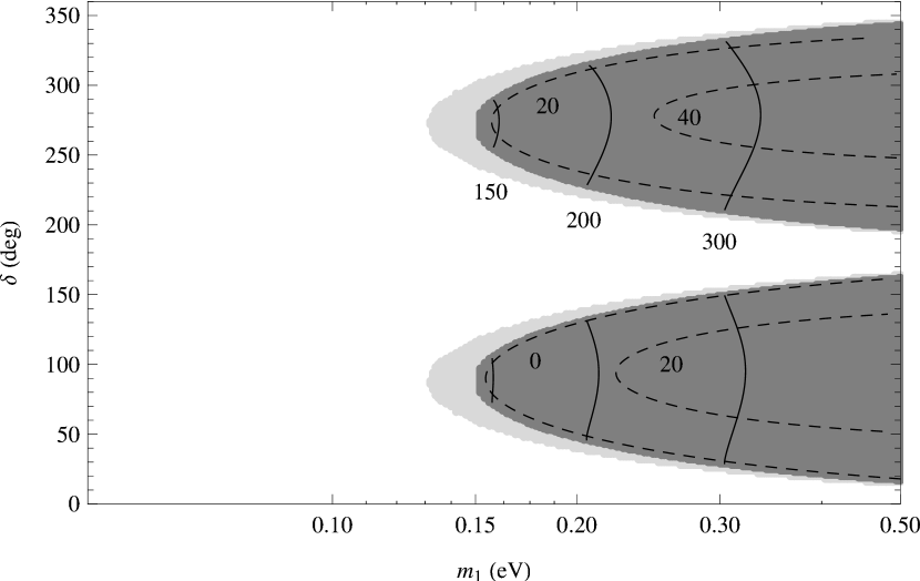
Figure 1: The allowed regions in the $(m_{1},\delta)$ plane for Class 1 and the normal ordering. The dark shaded regions correspond to the best-fit parameters of the oscillation parameters, while the light shaded regions are allowed at $2\sigma$. The solid lines are iso-$|M_{ee}|$ contours (in meV) and the dashed lines are iso-$\phi_{2}$ contours (in degrees).

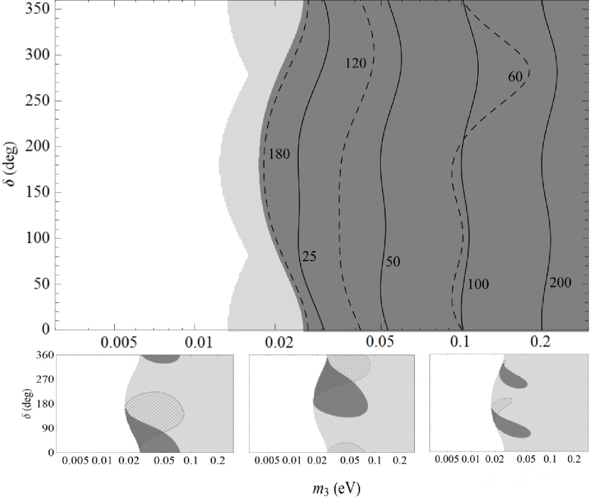
Figure 2: The upper panel shows the allowed regions in the $(m_{3},\delta)$ plane for Class 1 and the inverted ordering. The shading and line types in the upper panel are as in Fig. 1. The lower panels show the allowed regions for Class 1A and the inverted ordering with the additional constraint of successful single-flavored leptogenesis. The hatched (dark shaded) regions use the plus (minus) solution of $\phi_{2}$. From left to right the three graphs have the first, second and third row of $Y$ associated with the lightest right-handed neutrino mass, respectively.

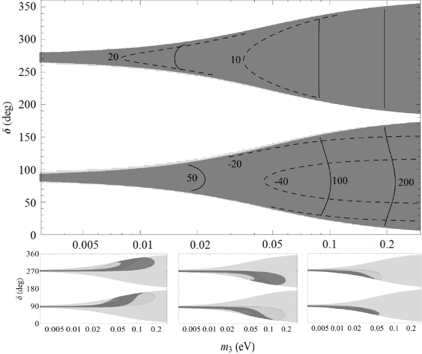
Figure 3: Same as Fig. 2, except for Class 2 and 2A and the inverted ordering.

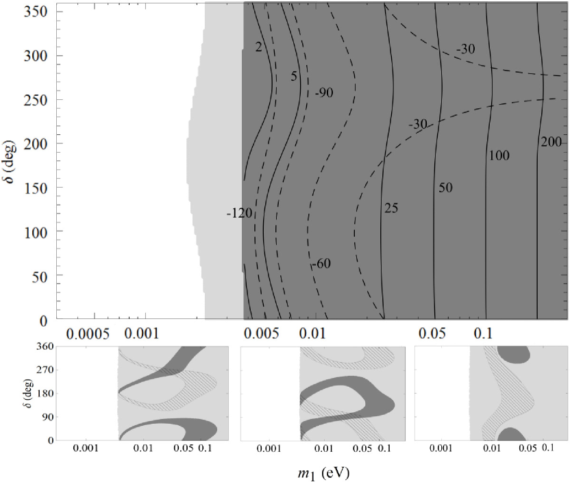
Figure 4: Same as Fig. 2, except for Class 3 and 3A and the normal ordering.

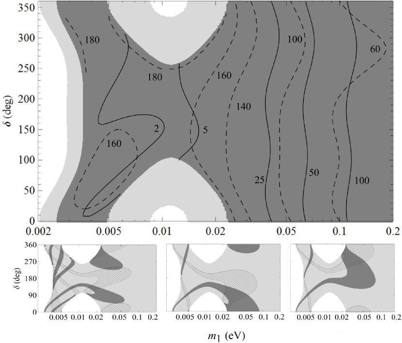
Figure 5: Same as Fig. 2, except for Class 4A and the normal ordering.

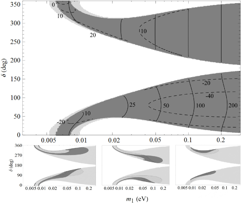
Figure 6: Same as Fig. 2, except for Class 4B and the normal ordering.

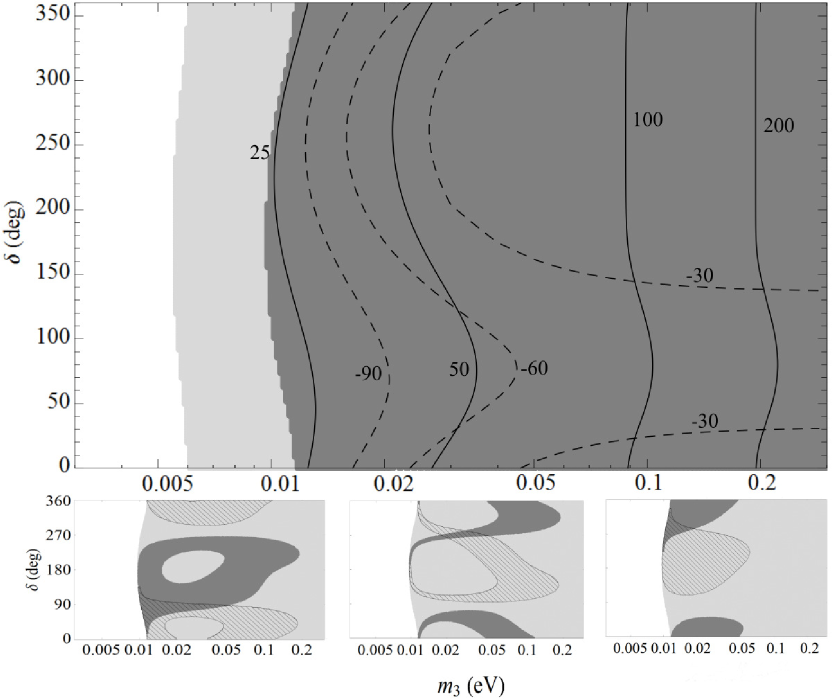
Figure 7: Same as Fig. 2, except for Class 4B and the inverted ordering.

Figure 8: The allowed regions in the $(|M_{ee}|,m_{3})$ plane for Class 2 and the inverted ordering. The dark shaded regions correspond to the best-fit parameters of the oscillation parameters, while the light shaded regions are allowed at $2\sigma$.

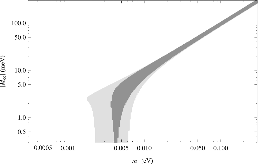
Figure 9: Same as Fig. 8, except for Class 3 and the normal ordering.

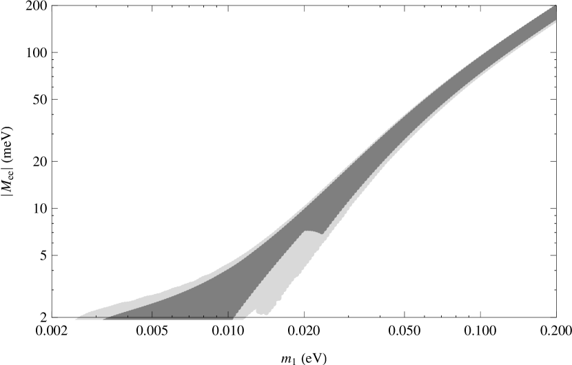
Figure 10: Same as Fig. 8, except for Class 4A and the normal ordering.

Figure 11: Same as Fig. 8, except for Class 4B and the inverted ordering.

References

- [1] J. Beringer et al. [Particle Data Group Collaboration], Phys. Rev. D 86, 010001 (2012).
- [2] F. P. An et al. [DAYA-BAY Collaboration], Phys. Rev. Lett. 108, 171803 (2012) [arXiv:1203.1669 [hep-ex]]; arXiv:1210.6327 [hep-ex].
- [3] J. K. Ahn et al. [RENO Collaboration], Phys. Rev. Lett. 108, 191802 (2012) [arXiv:1204.0626 [hep-ex]].
- [4] Y. Abe et al. [Double Chooz Collaboration], arXiv:1301.2948 [hep-ex].
- [5] G. L. Fogli, E. Lisi, A. Marrone, D. Montanino, A. Palazzo and A. M. Rotunno, Phys. Rev. D 86, 013012 (2012) [arXiv:1205.5254 [hep-ph]].
- [6] P. Minkowski, Phys. Lett. B 67 (1977) 421; T. Yanagida, in Proceedings of the Workshop on the Unified Theory and the Baryon Number in the Universe, eds. O. Sawada et al., (KEK Report 79-18, Tsukuba, 1979), p. 95; M. Gell-Mann, P. Ramond and R. Slansky, in Supergravity, eds. P. van Nieuwenhuizen et al., (North-Holland, 1979), p. 315; S.L. Glashow, in Quarks and Leptons, Cargèse, eds. M. L évy et al., (Plenum, 1980), p. 707; R. N. Mohapatra and G. Senjanović, Phys. Rev. Lett. 44 (1980) 912.
- [7] P. H. Frampton, S. L. Glashow and T. Yanagida, Phys. Lett. B 548, 119 (2002) [hep-ph/0208157].
- [8] K. Harigaya, M. Ibe and T. T. Yanagida, Phys. Rev. D 86, 013002 (2012) [arXiv:1205.2198 [hep-ph]].
- [9] G. C. Branco, D. Emmanuel-Costa, M. N. Rebelo and P. Roy, Phys. Rev. D 77, 053011 (2008) [arXiv:0712.0774 [hep-ph]].
- [10] M. Randhawa, G. Ahuja and M. Gupta, Phys. Rev. D 65, 093016 (2002) [hep-ph/0203109]; Z.-z. Xing and H. Zhang, Phys. Lett. B 569, 30 (2003) [hep-ph/0304234]; K. Matsuda and H. Nishiura, Phys. Rev. D 74, 033014 (2006) [hep-ph/0606142]; G. Ahuja, S. Kumar, M. Randhawa, M. Gupta and S. Dev, Phys. Rev. D 76, 013006 (2007) [hep-ph/0703005 [hep-ph]]; S. Choubey, W. Rodejohann and P. Roy, Nucl. Phys. B 808, 272 (2009) [Erratum-ibid. 818, 136 (2009)] [arXiv:0807.4289 [hep-ph]]; B. Adhikary, A. Ghosal and P. Roy, JHEP 0910, 040 (2009) [arXiv:0908.2686 [hep-ph]]; S. Dev, S. Kumar, S. Verma, S. Gupta and R. R. Gautam, Eur. Phys. J. C 72, 1940 (2012) [arXiv:1203.1403 [hep-ph]]; J. Barranco, D. Delepine and L. Lopez-Lozano, Phys. Rev. D 86, 053012 (2012) [arXiv:1205.0859 [hep-ph]]; B. Adhikary, M. Chakraborty and A. Ghosal, Phys. Rev. D 86, 013015 (2012) [arXiv:1205.1355 [hep-ph]]; M. Gupta and G. Ahuja, Int. J. Mod. Phys. A 26, 2973 (2011) [arXiv:1206.3844 [hep-ph]]; B. Adhikary and P. Roy, Adv. High Energy Phys. 2013, 324756 (2013) [arXiv:1211.0371 [hep-ph]].
- [11] M. Auger et al. [EXO Collaboration], Phys. Rev. Lett. 109, 032505 (2012) [arXiv:1205.5608 [hep-ex]].
- [12] W. Rodejohann, J. Phys. G 39, 124008 (2012) [arXiv:1206.2560 [hep-ph]].
- [13] S. Blanchet and P. Di Bari, New J. Phys. 14, 125012 (2012) [arXiv:1211.0512 [hep-ph]].
- [14] G. F. Giudice, A. Notari, M. Raidal, A. Riotto and A. Strumia, Nucl. Phys. B 685, 89 (2004) [hep-ph/0310123].
- [15] E. Komatsu et al. [WMAP Collaboration], Astrophys. J. Suppl. 192, 18 (2011) [arXiv:1001.4538 [astro-ph.CO]].