Single Dirac-Cone State and Quantum Hall Effects in Honeycomb Structure

Abstract

A honeycomb lattice system has four types of Dirac electrons corresponding to the spin and valley degrees of freedom. We consider a state that contains only one type of massless electrons and three types of massive ones, which we call the single Dirac-cone state. We analyze quantum Hall (QH) effects in this state. We make a detailed investigation of the Chern and spin-Chern numbers. We make clear the origin of unconventional QH effects discovered in graphene. We also show that the single Dirac-cone state may have arbitrary large spin-Chern numbers in magnetic field. Such a state will be generated in antiferromagnetic transition-metal oxides under electric field or silicene with antiferromagnetic order under electric field.

Introduction: Dirac electrons on a honeycomb lattice have attracted much attention since the discovery of the unconventional quantum Hall (QH) effect in grapheneNovoselov ; Kim . Dirac electrons are ubiquitous in monolayer honeycomb systems, where there are four types of them corresponding to the spin and valley degrees of freedom. The spin-orbit (SO) interaction makes Dirac electrons massiveHaldane ; KaneMele ; LiuPRL . There are several materials possessing massive Dirac electrons. A remarkable property is that we are able to control the Dirac mass externally by applying electric fieldEzawaNJP , photo-irradiationOka09L ; Kitagawa ; EzawaPhoto and exchange interactionsRyu ; FengPNAS ; EzawaQAHE ; EzawaExM for some cases. We can even make one type of Dirac electrons massless and the other three massiveEzawaPhoto . This is an intriguing state invalidating the Nielsen-Ninomiya theoremNielsen , which requires an even number of massless Dirac fermions in the lattice system, by breaking the chiral symmetry. We have called such a state the single Dirac-cone (SDC) state. In this work we investigate the QHE in the SDC state and reveal some novel phenomena.

The unconventional QHE with Hall plateaux at the filling factor $\nu=\pm 2,\pm 6,\pm 10,\cdots$ implies the 4-fold degeneracy of each Landau level in graphene. The Hall conductivity increases by $e^{2}/h$ when the Fermi energy crosses one Landau level. If there were no degeneracy the Hall conductivity would be half-integer quantizedZheng ,

$$\sigma_{\text{H}}=\pm\frac{1}{2},\pm\frac{3}{2},\pm\frac{5}{2},\pm\frac{7}{2},\cdots,$$ (1)

in unit of $e^{2}/h$. However the "half integer" is hidden in graphene under the 4-fold degeneracy associated with the spin and valley degrees of freedomNovoselov ; Kim . There is a long history in quest for the genuine half-integer QHE given by (1). The SDC state might provide an answer to this problem since it has only one type of massless electrons and all nondegenerate massive electrons in general.

We start with exploring Hofstadter’s butterfly diagramsHatsugai93B ; Hatsugai ; Esaki ; Sato ; Hasegawa in a SDC state. We also analyze it in the low-energy Dirac theory, and find a good agreement between the results in the both theories in the low magnetic field regime. We calculate the Chern and spin-Chern numbers based on the bulk-edge correspondenceHatsugai93B in the lattice theory and based on the Kubo formulaGusynin95L in the Dirac theory. They show a perfect agreement in this regime. We note that the topological insulator is indexed by the Chern and spin-Chern numbers in external magnetic fieldSheng ; Prodan ; Yang , where the time-reversal symmetry is broken but the spin $s_{z}$ is a good quantum number. The spin-Chern number counts the Landau levels filled with the up-spin and the down-spin electrons.

We obtain two major findings. First, each type of electrons yields the Hall conductivity of the form (1) whether they are massless or massive, and the total series reads $\nu=0,\pm 1,\pm 2,\pm 3,\cdots$ with no degeneracy of each Landau level. No half-integer states appear. We also find that the QH states may have arbitrarily high spin-Chern numbers. Note that we only have $0,\pm 1$ in the conventional QHE. The physical reason to allow high spin-Chern numbers is that there are only spin poralized electrons near the Fermi level in the SDC state. A topological insulator possessing a high spin-Chern number has never been discussed in literature.

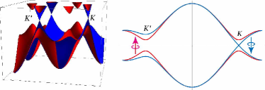
Figure 1: (a) Illustration of a SDC state. In this instance, down-spin (blue) electrons are massless at the K point but massive at the K’ point, while up-spin (red) electrons are massive both at the K and K’ points.

Hamiltonian: The honeycomb lattice consists of two sublattices made of $A$ sites and $B$ sites. We consider a buckled system with the layer separation $2\ell$ between these two sublattices. The states near the Fermi energy are $\pi$ orbitals residing near the $K$ and $K^{\prime}$ points at opposite corners of the hexagonal Brillouin zone. The low-energy dynamics in the $K$ and $K^{\prime}$ valleys is described by the Dirac theory. In what follows we use notations $s_{z}=\uparrow\downarrow$, $t_{z}=A,B$, $\eta=K,K^{\prime}$ in indices while $s_{z}^{\alpha}=\pm 1$ for $\alpha=\uparrow\downarrow$, $t_{z}^{i}=\pm 1$ for $i=A$,$B$, and $\eta_{i}=\pm 1$ for $i=K,K^{\prime}$ in equations. We also use the Pauli matrices $\sigma_{a}$ and $\tau_{a}$ for the spin and the sublattice pseudospin, respectively.

We investigate the system in perpendicular magnetic field $B$ by introducing the Peirls phase, $\Phi_{ij}=\frac{e}{h}\int_{\boldsymbol{r}_{i}}^{\boldsymbol{r}_{j}}\boldsymbol{A}\cdot d\boldsymbol{r}$, with $\boldsymbol{A}$ the magnetic potential. Any hopping term from site $i$ to site $j$ picks up the phase factor $e^{2\pi i\Phi_{ij}}$. The magnetic field is given by $B=2\Phi/3\sqrt{3}a^{2}$ in unit of $e/h$, where $a$ is the lattice constant and $\Phi$ is the magnetic flux penetrating one hexagonal area. Note that $\Phi=1$ implies $B=1.6\times 10^{5}$ Tesla in the case of graphene.

A generic Hamiltonian contains eight interaction terms mutually commutative in the Dirac limit. Among them four contribute to the Dirac mass. With the inclusion of those affecting the Dirac mass, the tight-binding model readsEzawaExM

$$H =-t\sum_{\left\langle i,j\right\rangle\alpha}e^{2\pi i\Phi_{ij}}c_{i\alpha}^{\dagger}c_{j\alpha}$$

$$+i\frac{\lambda_{\text{SO}}}{3\sqrt{3}}\sum_{\left\langle\!\left\langle i,j\right\rangle\!\right\rangle\alpha}s_{z}^{\alpha}e^{2\pi i\Phi_{ij}}\nu_{ij}c_{i\alpha}^{\dagger}c_{j\alpha}$$

$$+\lambda_{V}\sum_{i\alpha}t_{z}^{i}c_{i\alpha}^{\dagger}c_{i\alpha}+\lambda_{\text{SX}}\sum_{i\alpha}s_{z}^{\alpha}c_{i\alpha}^{\dagger}c_{i\alpha}$$

$$+i\frac{\lambda_{\text{H}}}{3\sqrt{3}}\sum_{\left\langle\!\left\langle i,j\right\rangle\!\right\rangle\alpha}e^{2\pi i\Phi_{ij}}\nu_{ij}c_{i\alpha}^{\dagger}c_{j\alpha},$$ (2)

where $\left\langle\!\left\langle i,j\right\rangle\!\right\rangle$ run over all the next-nearest neighbor hopping sites. We explain each term. The first term represents the usual nearest-neighbor hopping with the transfer energy $t\approx 1.6$eV. The second term represents the effective SO couplingKaneMele with $\lambda_{\text{SO}}\approx 3.9$meVLiuPRB , where $\nu_{ij}=\pm 1$ if the next-nearest-neighboring hopping is anticlockwise (clockwise) with respect to the positive $z$ axis. The third term represents the staggered sublattice potential term with $\lambda_{V}$ due to the bucked structureKaneMele . It may be present intrinsically as in boron-nitride and transition metal dichalcogenidesXiao ; Feng ; FengPNAS or generatedEzawaNJP externally by applying external electric field $E_{z}$, where $\lambda_{V}=\ell E_{z}$. The fourth term represents the staggered exchange termEzawaExM with the difference $\lambda_{\text{SX}}$ between the $A$ and $B$ sites. The fifth term is the Haldane termHaldane , which may be generated by photo irradiationOka09L ; Kitagawa ; EzawaPhoto .

The low-energy Dirac Hamiltonian at the $K$ point isEzawaExM

$$H_{\eta} = v_{\text{F}}\left(\eta P_{x}\tau_{x}+P_{y}\tau_{y}\right)$$ (3)

$$+\lambda_{\text{SO}}\eta\tau_{z}\sigma_{z}-\lambda_{V}\tau_{z}+\lambda_{\text{SX}}\sigma_{z}\tau_{z}+\eta\lambda_{\text{H}}\tau_{z},$$

where $v_{\text{F}}=\frac{\sqrt{3}}{2}at$ is the Fermi velocity, and $P_{i}\equiv\hbar k_{i}+eA_{i}$ is the covariant momentum. When the spin $s_{z}$ is diagonalized, the term

$$\Delta_{s_{z}}^{\eta}=\eta s_{z}\lambda_{\text{SO}}-\lambda_{V}+s_{z}\lambda_{\text{SX}}+\eta\lambda_{\text{H}}$$ (4)

becomes the mass of Dirac electrons with $2|\Delta_{s_{z}}^{\eta}|$ being the gap at the $K_{\eta}$ point with the spin $s_{z}$.

Single Dirac-Cone States: We can make a full control of the Dirac mass independently at each spin and valley. For instance, we may choose the parameters so that

$$\Delta_{\downarrow}^{K}=0\text{ with all other }\Delta_{s_{z}}^{\eta}\neq 0,$$ (5)

which generates the SDC state as in Fig.1(a). The band structure of a zigzag nanoribbon at $\Phi=0$ is illustrated in Fig.2(a), where there appear only down-spin electrons near the Fermi level at the $K$ point.

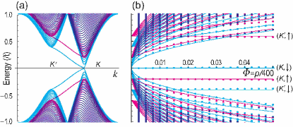
Figure 2: (a) The band structure of a zigzag nanoribbon at $\Phi=0$. There exists only up-spin electrons near the Fermi level. We have set $\lambda_{\text{SO}}=0.2t$ and $\lambda_{\text{SX}}=-0.3t$ and $\lambda_{V}=0.1t$ for illustration. The horizontal axis is the momentum $k$. (b) A closer look of the Hofstadter’s butterfly for $\Phi=p/400$ with $p=1,2,\cdots,20$, and the Fan diagram of Landau levels derived in the Dirac theory. The horizontal axis is the magnetic flux $\Phi$.

Fan Diagram: We introduce a pair of Landau-level ladder operators,

$$\hat{a}=\frac{\ell_{B}(P_{x}+iP_{y})}{\sqrt{2}\hbar},\quad\hat{a}^{\dagger}=\frac{\ell_{B}(P_{x}-iP_{y})}{\sqrt{2}\hbar},$$ (6)

satisfying $[\hat{a},\hat{a}^{{\dagger}}]=1$, where $\ell_{B}=\sqrt{\hbar/eB}$ is the magnetic length. The Hamiltonian $H_{\eta}$ is block diagonal and given by

$$H_{\eta}=\left(\begin{array}[]{cc}H_{\uparrow}^{\eta}&0\\ 0&H_{\downarrow}^{\eta}\end{array}\right),$$ (7)

with the diagonal elements being

$$H_{s_{z}}^{\text{K}} = \left(\begin{array}[]{cc}\Delta_{s_{z}}^{\text{K}}\left(E_{z}\right)&\hbar\omega_{\text{c}}\hat{a}^{\dagger}\\ \hbar\omega_{\text{c}}\hat{a}&-\Delta_{s_{z}}^{\text{K}}\left(E_{z}\right)\end{array}\right),$$ (10)

$$H_{s_{z}}^{\text{K'}} = \left(\begin{array}[]{cc}\Delta_{s_{z}}^{\text{K'}}\left(E_{z}\right)&-\hbar\omega_{\text{c}}\hat{a}\\ -\hbar\omega_{\text{c}}\hat{a}^{\dagger}&-\Delta_{s_{z}}^{\text{K'}}\left(E_{z}\right)\end{array}\right)$$ (13)

in the basis $\left\{\psi_{A},\psi_{B}\right\}^{t}$.

It is straightforward to diagonalize the Hamiltonian $H_{s_{z}}^{\eta}$. The eigenvalues are $\pm E_{s_{z}}^{\eta}(N)$ with

$$E_{s_{z}}^{\eta}(N)=\sqrt{(\hbar\omega_{\text{c}})^{2}N+(\Delta_{s_{z}}^{\eta})^{2}},$$ (14a)

for $$N=1,2,\cdots \Phi$$, which depend on . We also have

$$E_{s_{z}}^{\eta}(0)=\eta\Delta_{s_{z}}^{\eta},$$ (14b)

corresponding to $N=0$, which is independent of $\Phi$: See Fig.2(b). The eigenstate describes electrons when $E_{s_{z}}^{\eta}>0$ and holes when $E_{s_{z}}^{\eta}<0$.

We refer to each energy spectrum $\pm E_{s_{z}}^{\eta}(N)$ together with $E_{s_{z}}^{\eta}(0)$ as a fan. There are four fans indexed by valley $K_{\eta}$ and spin $s_{z}$. Each fan consists of two parts, one for electrons and the other for holes. These two parts are connected at one pivot when $\Delta_{s_{z}}^{\eta}=0$, and otherwise one fan has two pivots. The separation between these two pivots is given by $2\Delta_{s_{z}}^{\eta}$, while the average distance of the two pivots from the Fermi level is given by $\mu_{s_{z}}^{\eta}$. Let us call the energy level (14b) the lowest Landau level. In this convention there exists one lowest Landau level in each fan. Thus there are four lowest Landau levels in one fan diagram.

We present the fan diagram for the SDC state in Fig.2(b). Four decomposed fans are visible since the four types of Dirac electrons have different masses $\Delta_{s_{z}}^{\eta}$ in the bulk spectrum [Fig.2(a)]. We see also four lowest Landau levels indexed by the spin and valley degrees of freedom ($K_{\eta},s_{z}$).

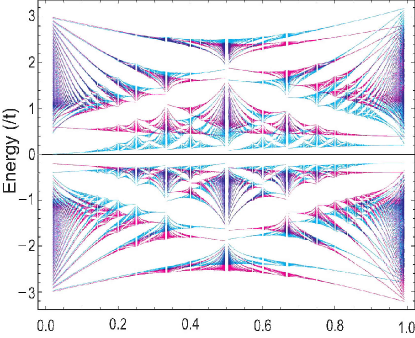
Figure 3: Spin-resolved Hofstadter’s diagram in a SDC state. We have set $\lambda_{\text{SO}}=0.2t$ and $\lambda_{\text{SX}}=-0.3t$ and $\lambda_{V}=0.1t$ for illustration. The contribution from up(down)-spin electrons is shown in magenta (cyan). The vertical axis is the energy in unit of $t$. The horizontal axis is the magnetic flux $\Phi$. We have taken $\Phi=p/q$ with $q\leq 100$.

Hofstadter Butterfly: We compute the bulk band structure numerically by applying periodic boundary conditions to the honeycomb system. This requires that the magnetic flux $\Phi$ to be a rational number, $\Phi=p/q$ ($p$ and $q$ are mutually prime integers). Then, the system is periodic in both spatial directions. We use the Bloch theorem to reduce the Schrödinger equation to a $2q\times 2q$ matrix equation for each $s_{z}=\uparrow\downarrow$, where the factor $2$ is due to the sublattice ($A$,$B$) degrees of freedom. In so doing we choose a generalized gauge of the one used in grapheneHatsugai93B so as to include the link connecting the next-nearest neighbor hopping sites. It is given in such a way that the magnetic flux becomes $1/6$ for each isosceles triangle whose two edges are given by the neighbor hopping.

The resulting band structure is the Hofstadters butterfly diagram, which we display for the SDC state in Fig.3. We present a closer look of the Hofstadter butterfly in the low magnetic field regime ($\Phi<5/100$) in Fig.2(b) together with the fan diagram. The spectra implied by the Hofstadter butterfly and the fan diagram agree one to another quite well for $\Phi<1/100$. The agreement is very good for the lowest and first Landau levels for a wide range of $\Phi$.

Topological Charges and Conductance: The Hall and spin-Hall conductivities are given by using the TKNN formulaTKNN ,

$$\sigma_{xy}=\frac{e^{2}}{2\pi\hbar}\mathcal{C},\qquad\sigma_{xy}^{\text{spin}}=\frac{e}{2\pi\hbar}\mathcal{C}_{\text{spin}},$$ (15)

where $\mathcal{C}$ and $\mathcal{C}_{\text{spin}}$ are the Chern number and the spin-Chern number, respectively. A topological insulator is indexed by a set of these two topological charges. When spin $s_{z}$ is a good quantum number, they are given by

$$\mathcal{C} = \mathcal{C}_{\uparrow}^{K}+\mathcal{C}_{\uparrow}^{K^{\prime}}+\mathcal{C}_{\downarrow}^{K}+\mathcal{C}_{\downarrow}^{K^{\prime}},$$ (16a)

$$\mathcal{C}_{\text{spin}} = \frac{1}{2}(\mathcal{C}_{\uparrow}^{K}+\mathcal{C}_{\uparrow}^{K^{\prime}}-\mathcal{C}_{\downarrow}^{K}-\mathcal{C}_{\downarrow}^{K^{\prime}}),$$ (16b)

where $\mathcal{C}_{s_{z}}^{\eta}$ is the summation of the Berry curvature in the momentum space over all occupied states of electrons with spin $s_{z}$ in the $K_{\eta}$ valley.

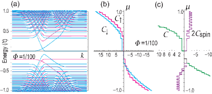
Figure 4: (a) The energy spectra of the honeycomb lattice with zigzag edges for $\Phi=1/100$. The horizontal axis is the momentum $k$. We can determine the topological number $\mathcal{C}_{s_{z}}$ by examining the edge modes. (b) The topological number $\mathcal{C}_{s_{z}}$ calculated based on the Kubo formula (18) as a function of $\mu$. The horizontal axis is the topological number $\mathcal{C}_{s}$. The results based on the bulk-edge correspondence (a) and the Kubo formula (b) are identical. (c) The Chern and spin-Chern numbers $\mathcal{C}$ (green) and $2\mathcal{C}_{\text{spin}}$ (violet) derived based on (16).

The most convenient way to determine the topological charge in the lattice formulation is to employ the bulk-edge correspondenceHatsugai93B . The edge-state analysis can be performed for a system with boundaries such as a cylinder. When solving the Harper equation on a cylinder, the spectrum consists of bulk bands and topological edge states as in Fig.4(a). We typically find a few edge states within the bulk gaps, some of which cross the gap from one bulk band to another. Each edge state contributes one unit to the quantum number $\mathcal{C}_{s_{z}}$ for each $s_{z}=\uparrow\downarrow$. More precisely, in order to evaluate $\mathcal{C}_{s_{z}}$, we count the edge states, taking into account their location (right or left edges) and direction (up or down) of propagationHatsugai93B . The location of each state is derived by computing the wave function, while the direction of propagation can be obtained from the sign of its momentum derivative $dE/dk$, with $k$ the momentum parallel to the edge.

We focus on one edge. Edge states with opposite directions contribute with opposite signs. The resultant formula reads

$$\mathcal{C}_{s_{z}}=N_{\text{u}}^{s_{z}}-N_{\text{d}}^{s_{z}},$$ (17)

where $N_{\text{u}}^{s_{z}}$ and $N_{\text{d}}^{s_{z}}$ denote the number of up- and down-moving states with spin $s_{z}$, respectively, at the right edge.

It is also possible to use the Kubo formulation in the Dirac theory to derive the Hall conductivity for each spin $s_{z}$ in each valley $K_{\eta}$. Such a formula has been derived for grapheneGusynin95L . We may generalize it and apply it to the Dirac system (3),

$$\mathcal{C}_{s_{z}}^{\eta}(\mu)= \frac{1}{4}\Big{[}\tanh\frac{\mu+\Delta_{s_{z}}^{\eta}}{2k_{\text{B}}T}+\tanh\frac{\mu-\Delta_{s_{z}}^{\eta}}{2k_{\text{B}}T}\Big{]}$$

$$+\frac{1}{2}\sum_{N=1}^{\infty}\Big{[}\tanh\frac{\mu+E_{s_{z}}^{\eta}(N)}{2k_{\text{B}}T}+\tanh\frac{\mu-E_{s_{z}}^{\eta}(N)}{2k_{\text{B}}T}\Big{]},$$ (18)

where $\mu$ is the chemical potential.

As a clear illustration we present the result of the edge-state analysis in magnetic field at $\Phi=1/100$ in Fig.4(a). According to the formula (17) we count the number of edge modes, from which we derive the topological numbers $\mathcal{C}_{\uparrow}^{N}$ (magenta) and $\mathcal{C}_{\downarrow}^{N}$ (cyan) based on (16). On the other hand we may calculate them from the Kubo formula (18), which we give in Fig.4(b). We can explicitly check that they agree one to another. The Chern and spin-Chern numbers $\mathcal{C}^{N}$ (blue) and $\mathcal{C}_{\text{spin}}^{N}$ (green) are calculated from $\mathcal{C}_{\uparrow}^{N}$ and $\mathcal{C}_{\downarrow}^{N}$ in Fig.4(c).

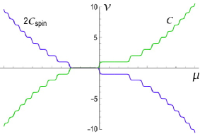
Figure 5: The Chern and spin-Chern numbers $\mathcal{C}$ (green) and $2\mathcal{C}_{\text{spin}}$ (violet) of the QH state for $B\lesssim 16$Tesla as a function of the chemical potential $\mu.$

The experimentally accessible regime is the low magnetic field limit $\Phi\lesssim 10^{-4}$ or $B\lesssim 16$Tesla. The prominent feature is that only the down-spin fan is present near the Fermi level both in the electron and hole sectors as in Fig.2(b). Consequently all the QH states are made of down-spin electrons near the Fermi level. They contribute equally to the Chern and spin-Chern numbers: It follows from (16) that $\mathcal{C}=\mathcal{C}_{\downarrow}^{K}=-2\mathcal{C}_{\text{spin}}$. As shown in Fig.5, the series of QH plateaux reads $\nu=0,\pm 1,\pm 2,\pm 3,\pm 4,\cdots$ with no degeneracy in each level, where the spin-Chern number reads

$$\mathcal{C}_{\text{spin}}=-\frac{1}{2}\nu.$$ (19)

The maximum value of $|\mathcal{C}_{\text{spin}}|$ increases as $\Phi$ becomes lower.

Discussions: Our analysis on the SDC state is applicable to any Dirac systems described by the Hamiltonian (2) or (3). Here we address the problem how to materialize a SDC state. Transition-metal oxide grown on [111] direction would be the first candidateHu . A salient property is that the material contains an intrinsic staggered exchange effect $\varpropto\lambda_{\text{SX}}$. It has antiferromagnetic order yielding a Dirac mass. We can control the band structure by applying electric field due to the buckled structure.

We may also consider silicene with antiferromagnetic order ($\lambda_{\text{SX}}\neq 0$) introduced by a proximity coupling effect methodEzawaExM . Alternatively we may apply photo irradiationEzawaPhoto to produce the Haldane term ($\lambda_{\text{H}}\neq 0$). In so doing it is necessary to arrange that transitions between Landau levels within the conduction band as well as between the valence and conduction bands (interband transitions) are prohibitted. This would be possible if we use photo-irradiation with frequency $\omega$ such that $\hbar\omega>3$eV since the Landau levels are bounded within this range as in Fig.3.

Conclusions: We have analyzed the QH effects in the SDC state. We conclude that no half-integer QH states appear because there are four types of electrons each of which contributes the basic series (1) whether they are massless or massive. This must be the case in any lattice theory since the number of electron types is even whether they are massless or massive. We have also found that the SDC state has arbitrarily high spin-Chern numbers in magnetic field.

I am very much grateful to N. Nagaosa, H. Aoki and Y. Hatsugai for many fruitful discussions on the subject. This work was supported in part by Grants-in-Aid for Scientific Research from the Ministry of Education, Science, Sports and Culture No. 22740196.

References

- (1) K. S. Novoselov, A. K. Geim, S. V. Morozov, D. Jiang, M. I. Katsnelson, I. V. Grigorieva, S. V. Dubonos, and A. A. Firsov, Nature 438, 360 (2005).
- (2) Y. Zhang, Y. W. Tan, H. L. Stormer and P. Kim, Nature 438, 201 (2005).
- (3) F. D. M. Haldane, Phys. Rev. Lett. 61, 2015 (1988).
- (4) C. L. Kane and E. J. Mele, Phys. Rev. Lett. 95, 226801 (2005).
- (5) C.-C. Liu, W. Feng, and Y. Yao, Phys. Rev. Lett. 107, 076802 (2011).
- (6) M. Ezawa, New J. Phys. 14, 033003 (2012).
- (7) T. Oka and H. Aoki, Phys. Rev. B 79, 081406(R) (2009).
- (8) T. Kitagawa, T. Oka, A. Brataas, L. Fu, and E. Demler, Phys. Rev. B 84, 235108 (2011).
- (9) M. Ezawa, Phys. Rev. Lett. 110, 026603 (2013).
- (10) S. Ryu, C. Mudry, C.Y. Hou and C. Chamon, Phys. Rev. B 80, 205319 (2009).
- (11) X. Li, T. Cao, Q. Niu, J. Shin and J. Feng, PNAS 110, 3738 (2013)
- (12) M. Ezawa, Phys. Rev. Lett 109, 055502 (2012).
- (13) M. Ezawa, Phys. Rev. B 87, 155415 (2013)
- (14) H.B. Nielsen, M. Ninomiya, Nucl.Phys. B 185 20 (1981).
- (15) Y. Zheng and T. Ando, Phys. Rev. B 65, 245420 (2002).
- (16) Y. Hatsugai, Phys. Rev. B 48, 11851 (1993).
- (17) Y. Hatsugai, T. Fukui and H. Aoki, Phys. Rev. B 74 205414 (2006).
- (18) K. Esaki, M. Sato, M. Kohmoto, and B. I. Halperin, Phys. Rev. B 80 125405 (2009).
- (19) M. Sato, D. Tobe and M. Kohmoto, Phys. Rev. B 78 235322 (2008).
- (20) Y. Hasegawa and M. Kohmoto, Phys. Rev. B 74 155415 (2006).
- (21) V.P. Gusynin, S.G. Sharapov, Phys. Rev. Lett. 95, 146801 (2005): Phys. Rev. B 73, 245411 (2006).
- (22) D. N. Sheng, Z. Y. Weng, L. Sheng, and F. D. M. Haldane, Phys. Rev. Lett. 97, 036808 (2006).
- (23) E. Prodan, Phys. Rev. B 80, 125327 (2009).
- (24) Y. Yang, Z. Xu, L. Sheng, B. Wang, D.Y. Xing, and D. N. Sheng, Phys. Rev. Lett. 107, 066602 (2011).
- (25) C.-C. Liu, H. Jiang, and Y. Yao, Phys. Rev. B, 84, 195430 (2011).
- (26) D. Xiao, G.-B. Liu, W. Feng, X. Xu, and W. Yao, Phys. Rev. Lett. 108, 196802 (2012).
- (27) T. Cao, G. Wang, W. Han, H. Ye, C. Zhu, J. Shi, Q. Niu, P. Tan, E. Wang, B. Liu and J. Feng, Nature Communications 3, 887 (2012).
- (28) D. J. Thouless, M. Kohmoto, M. P. Nightingale, and M. den Nijs, Phys. Rev. Lett. 49, 405 (1982).
- (29) Q.-F. Liang, L.-H. Wu, X. Hu, New J. Phys. 15 063031 (2013).