Semiclassical inverse spectral theory for singularities of focus-focus type

Abstract.

We prove, assuming that the Bohr-Sommerfeld rules hold, that the joint spectrum near a focus-focus critical value of a quantum integrable system determines the classical Lagrangian foliation around the full focus-focus leaf. The result applies, for instance, to $\hbar$-pseudodifferential operators, and to Berezin-Toeplitz operators on prequantizable compact symplectic manifolds.

1. Introduction

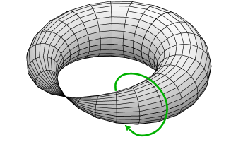
Figure 2. Fiber containing a focus-focus singularity.

The development of semiclassical and microlocal analysis since the 1960’s now provides a strong theoretical background to discover new interactions between spectral theoretic and analytic methods, and geometric and dynamical ideas from symplectic geometry (see for instance Guillemin-Sternberg [12] and Zworski [25]). The theme of this paper is to study these interactions for an important class of singularities which appear in integrable systems: focus-focus singularities (of the associated Lagrangian foliation). The singular fibers corresponding to such singularities are pinched tori (Figure 2). Focus-focus singularities appear naturally also in algebraic geometry in the context of Lefschetz fibrations, where they are sometimes called nodes.

In this article we consider the joint spectrum of a pair of commuting semiclassical operators, in the case where the phase space is fourdimensional. We prove, assuming that the Bohr-Sommerfeld rules hold, that the joint spectrum in a neighborhood of a focus-focus singularity determines the classical dynamics of the associated system around the focus-focus fiber. This problem belongs to a class of inverse spectral questions which has attracted much attention in recent years, eg. [13, 6], and which goes back to pioneer works of Colin de Verdière [4, 5] and Guillemin-Sternberg [11], in the 1970s and 1980s.

The result applies as soon as one can show that the usual Bohr-Sommerfeld rules hold for the quantum system. This includes the cases of $\hbar$-semiclassical pseudodifferential operators, as shown in [1] and [19]; it also includes the interesting case of Berezin-Toeplitz quantization, see [2].

Examples of quantum integrable systems, given by differential operators, with precisely one singularity of focus-focus type are the spherical pendulum, discussed by Cushman and Duistermaat in [7] (see also [21, Chapitre 2]), and the “Champagne bottle” [3]. Integrable systems given by Berezin-Toeplitz quantization are also common in the physics literature. An important example is the coupling of angular momenta (spins) [16] (see also [14, Section 8.3] for a proof that it is indeed a Berezin-Toeplitz system).

Many other integrable systems have focus-focus singularities, which are in fact the simplest integrable singularity with an isolated critical value. An infinite number of non-isomorphic systems with focus-focus singularities are provided by the so called semitoric systems constructed in [15].

The structure of the paper is as follows: in Section 2 we explain what we mean by a semiclassical operator, and recall the notion of integrable system in dimension four. In Section 3 we state our main theorem: Theorem 3.3. In Section 4 we review the construction of the so called Taylor series invariant, which classifies, up to isomorphisms, a semiglobal neighborhood of a focus-focus singularity. In Section 5 we prove Theorem 3.3.

2. Symplectic theory of integrable systems

Let $(M,\omega)$ be a smooth, connected $4$-dimensional symplectic manifold.

2.1. Integrable systems

An integrable system $(J,H)$ on $(M,\omega)$ consists of two Poisson commuting functions $J,H\in\!\!\mathop{\rm~{}C}\nolimits^{\infty}(M;\mathbb{R})$ i.e. :

$$\{J,H\}:=\omega(\mathcal{X}_{J},\,\mathcal{X}_{H})=0,$$

whose differentials are almost everywhere linearly independent $1$-forms. Here $\mathcal{X}_{J},\mathcal{X}_{H}$ are the Hamiltonian vector fields induced by $J,H$, respectively, via the symplectic form $\omega$: $\omega(\mathcal{X}_{J},\cdot)=-{\rm d}J$, $\omega(\mathcal{X}_{H},\cdot)=-{\rm d}H$.

For instance, let $M_{0}={\rm T}^{*}{\mathbb{T}}^{2}$ be the cotangent bundle of the torus ${\mathbb{T}}^{2}$, equipped with canonical coordinates $(x_{1},x_{2},\xi_{1},\xi_{2})$, where $x\in{\mathbb{T}}^{2}$ and $\xi\in{\rm T}^{*}_{x}{\mathbb{T}}^{2}$. The linear system

$$(J_{0},H_{0}):=(\xi_{1},\xi_{2})$$

is integrable.

An isomorphism of integrable systems $(J,\,H)$ on $(M,\omega)$ and $(J^{\prime},\,H^{\prime})$ on $(M^{\prime},\omega^{\prime})$ is a diffeomorphism $\varphi\colon M\to M^{\prime}$ such that $\varphi^{*}\omega^{\prime}=\omega$ and

$$\varphi^{*}(J^{\prime},\,H^{\prime})=(f_{1}(J,\,H),\,f_{2}(J,\,H))$$

for some local diffeomorphism $(f_{1},f_{2})$ of ${\mathbb{R}}^{2}$. This same definition of isomorphism extends to any open subsets $U\subset M$, $U^{\prime}\subset M^{\prime}$ (and this is the form in which we will use it later). Such an isomorphism will be called semiglobal if $U,U^{\prime}$ are respectively saturated by level sets $\{J=\text{const}_{1},H=\text{const}_{2}\}$ and $\{J^{\prime}=\text{const}^{\prime}_{1},H^{\prime}=\text{const}^{\prime}_{2}\}$.

If $F=(J,H)$ is an integrable system on $(M,\omega)$, consider a point $c\in{\mathbb{R}}^{2}$ that is a regular value of $F$, and such that the fiber $F^{{-1}}(c)$ is compact and connected. Then, by the action-angle theorem [8], a saturated neighborhood of the fiber is isomorphic in the previous sense to the above linear model on $M_{0}={\rm T}^{*}{\mathbb{T}}^{2}$. Therefore, all such regular fibers (called Liouville tori) are isomorphic in a neighborhood.

However, the situation changes drastically when the condition that $c$ be regular is violated. For instance, it has been proved in [20] that, when $c$ is a so-called focus-focus critical value (see Section 2.2 below), an infinite number of equations has to be satisfied in order for two systems to be semiglobally isomorphic near the critical fiber (see Section 4).

2.2. Focus-focus singularities

Let $\mathcal{F}$ be the associated singular foliation to the integrable system $F=(J,\,H)\colon M\to{\mathbb{R}}^{2}$, the leaves of which are by definition the connected components of the fibers $F^{-1}(c)$. Let $p$ be a critical point of $F$. We assume for simplicity that $F(p)=0$, and that the (compact, connected) fiber $\Lambda_{0}:=F^{-1}(0)$ does not contain other critical points. A focus-focus singularity $p$ is characterized by Eliasson’s theorem [10, 22] as follows: there exist symplectic coordinates $(x,\,y,\,\xi,\,\eta)$ in a neighborhood $W$ around $p$ in which $(q_{1},\,q_{2})$, given by

(1) $$q_{1}=x\eta-y\xi,\,\,q_{2}=x\xi+y\eta$$

is a momentum map for the foliation $\mathcal{F}$: one has $F=g(q_{1},q_{2})$ for some local diffeomorphism $g$ of ${\mathbb{R}}^{2}$ defined near the origin (the critical point $p$ corresponds to coordinates $(0,\,0,\,0,\,0)$). One of the major characteristics of focus-focus singularities is the existence of a Hamiltonian action of $S^{1}$ that commutes with the flow of the system, in a neighborhood of the singular fiber that contains $p$ [24, 23]. Such singularities are also very natural candidates for a topological study of singular Lagrangian fibrations [17].

3. Main Theorem: inverse spectral theory for focus-focus singularities

Let $(M,\omega)$ be a $4$-dimensional connected symplectic manifold.

3.1. Semiclassical operators

Let $I\subset(0,1]$ be any set which accumulates at $0$. If $\mathcal{H}$ is a complex Hilbert space, we denote by $\mathcal{L}(\mathcal{H})$ the set of linear (possibly unbounded) selfadjoint operators on $\mathcal{H}$ with a dense domain.

A space $\Psi$ of semiclassical operators is a subspace of $\prod_{\hbar\in I}\mathcal{L}(\mathcal{H}_{\hbar})$ equipped with a ${\mathbb{R}}$-linear map

$$\sigma\colon\Psi\to{\rm C}^{\infty}(M;\,{\mathbb{R}}),$$

called the principal symbol map. If $P=(P_{\hbar})_{\hbar\in I}\in\Psi$, the image $\sigma(P)$ is called the principal symbol of $P$.

We say that two semiclassical operators $(P_{\hbar})_{\hbar\in I}$ and $(Q_{\hbar})_{\hbar\in I}$ commute if for each $\hbar\in I$ the operators $P_{\hbar}$ and $Q_{\hbar}$ commute.

3.2. Semiclassical spectrum

Let $P=(P_{\hbar})_{\hbar\in I}$ and $Q=(Q_{\hbar})_{\hbar\in I}$ be semiclassical commuting operators on Hilbert spaces $(\mathcal{H}_{\hbar})_{\hbar\in I}$, where at each $\hbar\in I$ the operators have a common dense domain $\mathcal{D}_{\hbar}\subset\mathcal{H}_{\hbar}$ such that $P_{\hbar}(\mathcal{D}_{\hbar})\subset\mathcal{D}_{\hbar}$ and $Q_{\hbar}(\mathcal{D}_{\hbar})\subset\mathcal{D}_{\hbar}$.

For fixed $\hbar$, the joint spectrum of $(P_{\hbar},Q_{\hbar})$ is the support of the joint spectral measure (see Figure 1 for an example). It is denoted by $\!\!\mathop{\rm~{}JointSpec}\nolimits(P_{\hbar},\,Q_{\hbar})$. If $\mathcal{H}_{\hbar}$ is finite dimensional, then

$$\!\!\mathop{\rm~{}JointSpec}\nolimits(P_{\hbar},\,Q_{\hbar})=\Big{\{}(\lambda_{1},\lambda_{2})\in{\mathbb{R}}^{2}\,\,|\,\,\exists v\neq 0,\,\,P_{\hbar}v=\lambda_{1}v,\,\,Q_{\hbar}v=\lambda_{2}v\Big{\}}.$$

The joint spectrum of $P,Q$ is the collection of all joint spectra of $(P_{\hbar},Q_{\hbar})$, $\hbar\in I$. It is denoted by $\!\!\mathop{\rm~{}JointSpec}\nolimits(P,\,Q)$. For convenience of the notation, we will also view the joint spectrum of $P,Q$ as a set depending on $\hbar$.

3.3. Bohr-Sommerfeld rules

Recall that the Hausdorff distance between two subsets $A$ and $B$ of ${\mathbb{R}}^{2}$ is

$${\rm d}_{H}(A,\,B):=\inf\{\epsilon>0\,\,|\,\ A\subseteq B_{\epsilon}\ \mbox{and}\ B\subseteq A_{\epsilon}\},$$

where for any subset $X$ of ${\mathbb{R}}^{2}$, the set $X_{\epsilon}$ is

$$X_{\epsilon}:=\bigcup_{x\in X}\{m\in{\mathbb{R}}^{2}\,\,|\,\,\|x-m\|\leqslant\epsilon\}.$$

If $(A_{\hbar})_{\hbar\in I}$ and $(B_{\hbar})_{\hbar\in I}$ are sequences of subsets of $\mathbb{R}^{2}$, we say that

$$A_{\hbar}=B_{\hbar}+\mathcal{O}(\hbar^{N})$$

if there exists a constant $C>0$ such that

$${\rm d}_{H}(A_{\hbar},\,B_{\hbar})\leqslant C\hbar^{N}$$

for all $\hbar\in I$.

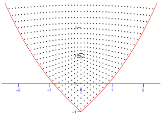
Figure 1. Joint spectrum of the quantum spherical pendulum when $\hbar=\frac{1}{10}$ (figure taken from [21]).

Definition 3.1. Let $F:=(J,H)\colon M\to\mathbb{R}^{2}$ be an integrable system on a $4$-dimensional connected symplectic $4$-manifold. Let $P$ and $Q$ be commuting semiclassical operators with principal symbols $J,H\colon M\to\mathbb{R}$. Let $U\subset\mathbb{R}^{2}$ be an open set. We say that $\!\!\mathop{\rm~{}JointSpec}\nolimits(P,\,Q)$ satisfies the Bohr-Sommerfeld rules on $U$ if for every regular value $c\in U$ of $F$ there exists a small ball ${\rm B}(c,\epsilon_{c})\subset U$ centered at $c$ such that

$$\!\!\mathop{\rm~{}JointSpec}\nolimits(P,\,Q)\cap{\rm B}(c,\epsilon_{c})=g_{\hbar}(2\pi\hbar{\mathbb{Z}}^{2}\cap D)\cap{\rm B}(c,\epsilon_{c})+\mathcal{O}(\hbar^{2})$$

with

$$g_{\hbar}=g_{0}+\hbar g_{1},$$

where $g_{0},g_{1}$ are smooth maps defined on a bounded open set $D\subset{\mathbb{R}}^{2}$, $g_{0}$ is a diffeomorphism into its image, and the components of $g_{0}^{-1}=(\mathcal{A}_{1},\,\mathcal{A}_{2})$ form a basis of action variables. We call $(g_{\hbar})^{-1}$ an affine chart for $\!\!\mathop{\rm~{}JointSpec}\nolimits(P,\,Q)$.

For instance, Bohr-Sommerfeld rules are known to hold for pseudodifferential operators on cotangent bundles [1, 19], or for Toeplitz operators on prequantizable compact symplectic manifolds [2]. It would be interesting to formalize the minimal semiclassical category where Bohr-Sommerfeld rules are valid.

Remark 3.2. If $(g_{\hbar})^{-1}$ is an affine chart for ${\rm JointSpec}(P,Q)$ and $B\in{\rm GL}(2,{\mathbb{Z}})$ then $B\circ(g_{\hbar})^{-1}$ is again an affine chart.

3.4. Main Theorem

Let ${\rm CIS}(M,\omega)$ be the set of classical integrable systems

$$F=(J,H)\colon M\to\mathbb{R}^{2}$$

on the connected $4$-dimensional symplectic manifold $(M,\omega)$, such that $F$ is a proper map. Let ${\rm QIS}(M,\omega)$ be the set of quantum integrable systems given as pairs of commuting semiclassical operators $(P,Q)$ whose principal symbols, say $(J,H)=\sigma(P,Q)$, form an integrable system $F\in{\rm CIS}(M,\omega)$. Let $\mathcal{P}({\mathbb{R}}^{2})$ the set of subsets of ${\mathbb{R}}^{2}$, and consider the following diagram:

(6)

Theorem 3.3.

Let $(M,\omega)$ and $(M^{\prime},\omega^{\prime})$ be connected $4$-dimensional symplectic manifolds. Let $(P,Q)$ and $(P,Q^{\prime})$ be quantum integrable systems on $(M,\omega)$ and $(M^{\prime},\omega^{\prime})$, respectively, which have a focus-focus singularity at points $p\in M$ and $p^{\prime}\in M^{\prime}$ respectively. Suppose that $c_{0}:=\sigma(P,Q)(p)=\sigma(P^{\prime},Q^{\prime})(p^{\prime})$ and that there exists a neighborhood $U$ of $c_{0}$ such that ${\rm JointSpec}(P,Q)$ and ${\rm JointSpec}(P^{\prime},Q^{\prime})$ satisfy the Bohr-Sommerfeld rules on $U$. If

$${\rm JointSpec}(P,Q)\cap U=({\rm JointSpec}(P^{\prime},Q^{\prime})\cap U)+\mathcal{O}(\hbar^{2}),$$

then there are saturated neighborhoods $\mathcal{V},\mathcal{V}^{\prime}$ of the singular fibers of $\sigma(P,Q)$ and $\sigma(P^{\prime},Q^{\prime})$ respectively, such that the restrictions $\sigma(P,Q)|_{\mathcal{V}}$ and $\sigma(P^{\prime},Q^{\prime})|_{\mathcal{V^{\prime}}}$ are isomorphic as integrable systems.

4. Taylor series invariant at focus-focus singularity

We use here the notation of Section 2.2. In particular $p\in M$ is a focus-focus point, and $W$ is a small neighborhood of $p$. Fix $A^{\prime}\in\Lambda_{0}\cap(W\setminus\{p\})$ and let $\Sigma$ denote a small 2-dimensional surface transversal to $\mathcal{F}$ at the point $A^{\prime}$. Since the Liouville foliation in a small neighborhood of $\Sigma$ is regular for both $F$ and $q=(q_{1},\,q_{2})$, there is a diffeomorphism $\varphi$ from a neighborhood $U$ of $F(A^{\prime})\in{\mathbb{R}}^{2}$ into a neighborhood of the origin in ${\mathbb{R}}^{2}$ such that $q=\varphi\circ{F}$. Thus there exists a smooth momentum map $\Phi=\varphi\circ{F}$ for the foliation, defined on a neighborhood $\Omega=F^{-1}(U)$ of $\Lambda_{0}$, which agrees with $q$ on $W$. Write $\Phi:=(H_{1},\,H_{2})$ and $\Lambda_{c}:=\Phi^{-1}(c)$. Note that $\Lambda_{0}=\mathcal{F}_{p}.$ It follows from (1) that near $p$ the $H_{1}$-orbits must be periodic of primitive period $2\pi$, whereas the vector field $\mathcal{X}_{H_{2}}$ is hyperbolic with a local stable manifold (the $(\xi,\eta)$-plane) transversal to its local unstable manifold (the $(x,y)$-plane). Moreover, $\mathcal{X}_{H_{2}}$ is radial, meaning that the flows tending towards the origin do not spiral on the local (un)stable manifolds.

Suppose that $A\in\Lambda_{c}$ for some regular value $c$.

Definition 4.1. Let $\tau_{2}(c)>0$ be the smallest time it takes the Hamiltonian flow associated with $H_{2}$ leaving from $A$ to meet the Hamiltonian flow associated with $H_{1}$ which passes through $A$. Let $\tau_{1}(c)\in[0,2\pi)$ be the time that it takes to go from this intersection point back to $A$, closing the trajectory.

In Definition 4, the existence of $\tau_{2}$ is ensured by the fact that the flow of $H_{2}$ is a quasiperiodic motion always transversal to the $S^{1}$-orbits generated by $H_{1}$.

The commutativity of the flows ensure that $\tau_{1}(c)$ and $\tau_{2}(c)$ do not depend on the initial point $A$.

Write $c=(c_{1},\,c_{2})=c_{1}+\!\!\mathop{\rm~{}i}\nolimits c_{2}$ ($c_{1},\,c_{2}\in{\mathbb{R}}$), and let $\!\!\mathop{\rm~{}log}\nolimits c$ be a fixed determination of the logarithmic function on the complex plane. Let

(7) $$\left\{\begin{array}[]{ccl}\sigma_{1}(c)&=&\tau_{1}(c)-{\rm Im}(\!\!\mathop{\rm~{}log}\nolimits c)\\ \sigma_{2}(c)&=&\tau_{2}(c)+{\rm Re}(\!\!\mathop{\rm~{}log}\nolimits c),\end{array}\right.$$

where ${\rm Re}$ and ${\rm Im}$ respectively stand for the real and imaginary parts of a complex number. Vũ Ngọc proved in [20, Proposition  3.1] that $\sigma_{1}$ and $\sigma_{2}$ extend to smooth and single-valued functions in a neighborhood of $0$ and that the differential 1-form $\sigma:=\sigma_{1}\,\mathrm{d}{}c_{1}+\sigma_{2}\,\mathrm{d}{}c_{2}$ is closed. Notice that if follows from the smoothness of $\sigma_{1}$ that one may choose the lift of $\tau_{1}$ to ${\mathbb{R}}$ such that $\sigma_{1}(0)\in[0,\,2\pi)$. This is the convention used throughout.

Following [20, Definition 3.1] , let $S$ be the unique smooth function defined around $0\in{\mathbb{R}}^{2}$ such that

(8) $$\mathrm{d}{}S=\sigma,\,\,\,\,S(0)=0.$$

The Taylor expansion of $S$ at $(0,\,0)$ is denoted by $(S)^{\infty}$.

Definition 4.2. The expansion $(S)^{\infty}$ is a formal power series in two variables with vanishing constant term, and we call it the Taylor series invariant of $(J,\,H)$ at the focus-focus point $c_{0}$.

Theorem 4.3 ([20]).

The Taylor series invariant $(S)^{\infty}$ charaterizes, up to symplectic isomorphisms, a semiglobal saturated neighborhood of the singular fiber of the focus-focus singularity $p$.

It is interesting to notice that, in the famous case of the spherical pendulum, the Taylor series invariant was recently explicitly computed [9].

5. Proof of Theorem 3.3

In view of Theorem 4.3, we wish to prove that the symplectic invariant $(S)^{\infty}$ is determined by the joint spectrum. The proof is organized in several statements. Throughout we use the notation of Section 4. Let $(P,Q)\in{\rm QIS}(M,\omega)$ and $(P,Q^{\prime})\in{\rm QIS}(M^{\prime},\omega^{\prime})$ be quantum integrable systems which have a focus-focus singularity at points $p\in M$ and $p^{\prime}\in M^{\prime}$, respectively. Suppose that $c_{0}:=\sigma(P,Q)(p)=\sigma(P^{\prime},Q^{\prime})(p^{\prime})$ and that there exists a neighborhood $U$ of $c_{0}$ such that ${\rm JointSpec}(P,Q)$ and ${\rm JointSpec}(P^{\prime},Q^{\prime})$ satisfy the Bohr-Sommerfeld rules on $U$. Assume that

$${\rm JointSpec}(P,Q)\cap U=({\rm JointSpec}(P^{\prime},Q^{\prime})\cap U)+\mathcal{O}(\hbar^{2})$$

Let $\sigma(P,Q)=(J,H):=F\colon M\to\mathbb{R}^{2}$ and let $\sigma(P^{\prime},Q^{\prime})=(J^{\prime},H^{\prime}):=F^{\prime}\colon M^{\prime}\to\mathbb{R}^{2}$.

Lemma 5.1.

([18, Proposition 1]) Let $(f_{\hbar})^{-1}$ and $(g_{\hbar})^{-1}$ be two affine charts for ${\rm JointSpec}(P,Q)$, both defined on a ball $B$ around $c$. Let $(f_{0})^{-1},(g_{0})^{-1}$ denote the principal symbols of $(f_{\hbar})^{-1}$ and $(g_{\hbar})^{-1}$ respectively. Then there is a constant matrix $C\in{\rm GL}(2,{\mathbb{Z}})$ such that for all $c\in B$, we have that

$${\rm d}(g_{0})^{-1}(c)=C\cdot({\rm d}(f_{0})^{-1}(c)).$$

Proof.

We recall the proof for the reader’s convenience. Let $\Sigma_{\hbar}:={\rm JointSpec}(P_{\hbar},Q_{\hbar})$. Let $c\in U$, and $(f_{\hbar})^{-1}$, $(g_{\hbar})^{-1}$ be two affine charts of $\Sigma$ defined on a ball $B$ around $c$. Any open ball around $c$ contains, for $\hbar$ small enough, at least one element of $\Sigma_{\hbar}$. Therefore, there exists a family $\lambda_{\hbar}\in\Sigma_{\hbar}\cap B$ such that $\lim_{\hbar\to 0}\lambda_{\hbar}=c$. Let $k\in{\mathbb{Z}}^{2}$ and let $\lambda^{\prime}_{\hbar}$ be a family of elements of $\Sigma_{\hbar}\cap B$ such that

$$(f_{\hbar})^{-1}(\lambda_{\hbar})=(f_{\hbar})^{-1}(\lambda^{\prime}_{\hbar})+\hbar k+\mathcal{O}(\hbar^{2}).$$

Then, as $\hbar$ tends to zero, $\frac{\lambda^{\prime}_{\hbar}-\lambda_{\hbar}}{\hbar}$ tends towards a limit $v\in\mathbb{R}^{2}$ which satisfies $k={\rm d}(f_{0})^{-1}(c)v$. Since $\lambda_{\hbar}$ and $\lambda^{\prime}_{\hbar}$ are in $\Sigma_{\hbar}$, there is a family $k^{\prime}_{\hbar}\in{\mathbb{Z}}^{2}$ such that

(9) $$\left(\frac{(g_{\hbar})^{-1}(\lambda^{\prime}_{\hbar})-(g_{\hbar})^{-1}(\lambda_{\hbar})}{\hbar}\right)=k^{\prime}_{\hbar}+\mathcal{O}(\hbar).$$

The left-hand side of (9) has limit ${\rm d}(g_{0})^{-1}(c)v$ as $\hbar\to 0$. Therefore $k^{\prime}_{\hbar}$ is equal to a constant integer $k^{\prime}$ for small $\hbar$, and we have $k^{\prime}={\rm d}(g_{0})^{-1}(c)({\rm d}(f_{0})^{-1}(c))^{-1}k$, which implies that

$${\rm d}(g_{0})^{-1}(c)({\rm d}(f_{0})^{-1}(c))^{-1}\in{\rm GL}(2,{\mathbb{Z}}).$$

Since ${\rm GL}(2,{\mathbb{Z}})$ is discrete, the conclusion of the lemma follows. ∎

Next we proceed in several steps.

Step 1. First we normalize the systems $F:=(J,H)\colon M\to{\mathbb{R}}^{2}$ and $F^{\prime}:=(J^{\prime},H^{\prime})\colon M^{\prime}\to\mathbb{R}^{2}$ at the focus-focus singular points, which doesn’t change the Taylor series invariant. In order to do this, let $\varphi\colon\Omega\to({\mathbb{R}}^{4},\omega_{0})$ be a symplectomorphism into its image, where $\Omega$ is a neighborhood of the singular point $p$ and $\omega_{0}$ is the standard symplectic form on ${\mathbb{R}}^{4}$, such that $F\circ\varphi^{-1}=g(q_{1},q_{2})$ near $(0,0,0,0)$ (it exists by Eliasson’s Theorem, see Section 2.2). Here $g$ is some local diffeomorphism. Similarly let $\varphi^{\prime}\colon\Omega^{\prime}\to({\mathbb{R}}^{4},\omega_{0})$ be a local symplectomorphism, where $\Omega^{\prime}$ is a small neighborhood of the singular point $p^{\prime}$ such that $F^{\prime}\circ(\varphi^{\prime})^{-1}=g^{\prime}(q_{1},q_{2}).$ Here $g^{\prime}$ is some local diffeomorphism.

By replacing $F$ by the integrable system $g^{-1}\circ F$ and $F^{\prime}$ by $(g^{\prime})^{-1}\circ F^{\prime}$, defined respectively on semiglobal neighborhoods $\mathcal{V}$, $\mathcal{V}^{\prime}$ we may assume that $c_{0}=0$ and that $g$ and $g^{\prime}$ are both the identity near the origin, that is, we may assume that

$$F\circ\varphi^{-1}=(q_{1},q_{2}),\,\,\,\,\,\,\,\,\,\,F^{\prime}\circ(\varphi^{\prime})^{-1}=(q_{1},q_{2})$$

near $(0,0,0,0)$.

Step 2. Denote by ${\rm B}_{r}$ the set of regular values of $F$ and $F^{\prime}$ simultaneously. Since the focus-focus critical value $c_{0}=0$ is isolated, there exists a small ball $U$ around $0$ such that $\dot{U}:=U\setminus\{0\}={\rm B}_{r}\cap U$.

Let $c\in\dot{U}$; let $\Lambda_{c}:=F^{-1}(c)$, which is a Liouville torus. Let $(\delta_{1},\delta_{2})$ be loops in $\Lambda_{c}$ that form a basis of cycles in $H_{1}(\Lambda_{c},{\mathbb{R}})$. Let

$$\mathcal{A}_{j}(c)=\int_{\delta_{j}(c)}\nu,\,\,\,\,\,\,j=1,2$$

be the action integrals, where $\nu$ is a $1$-form such that $\mathrm{d}\nu=\omega$. Similarly, let $\Lambda^{\prime}_{c}:=(F^{\prime})^{-1}(c)$, let $(\delta^{\prime}_{1},\delta^{\prime}_{2})$ be a basis of cycles in $\Lambda^{\prime}_{c}$, and let

$$\mathcal{A}_{j}(c)=\int_{\delta^{\prime}_{j}(c)}\nu^{\prime},\,\,\,\,\,\,j=1,2.$$

Write $\mathcal{A}:=(\mathcal{A}_{1},\mathcal{A}_{2})$ and $\mathcal{A}^{\prime}:=(\mathcal{A}^{\prime}_{1},\mathcal{A}^{\prime}_{2})$. It follows from the action-angle theorem that $\mathcal{A}$ and $\mathcal{A}^{\prime}$ are local diffeomorphisms of ${\mathbb{R}}^{2}$ defined near $c$.

Lemma 5.2.

There exists a matrix $B\in{\rm GL}(2,{\mathbb{Z}})$ such that we have the following relation between the integrals above :

$$\mathcal{A}(c)=B\circ\mathcal{A}^{\prime}(c)+{\rm constant},$$

for all $c\in\dot{U}$.

Proof.

Fix $c\in\dot{U}$. Let $(g_{\hbar})^{-1},(g^{\prime}_{\hbar})^{-1}$ be affine charts near $c$ for the spectra ${\rm JointSpec}(P,Q)$ and ${\rm JointSpec}(P^{\prime},Q^{\prime})$ respectively. By Remark 1 we may assume that $(g_{0})^{-1}=(\mathcal{A}_{1},\mathcal{A}_{2})$ and $(g^{\prime}_{0})^{-1}=(\mathcal{A}^{\prime}_{1},\mathcal{A}^{\prime}_{2})$. Since the joint spectra are equal modulo $\mathcal{O}(\hbar^{2})$, $(g^{\prime}_{\hbar})^{-1}$ is also an affine chart for ${\rm JointSpec}(P,Q)$. Therefore by Lemma 5.1 there is a constant matrix $B\in{\rm GL}(2,{\mathbb{Z}})$ such that for all $c^{\prime}$ near $c$,

$${\rm d}(g_{0})^{-1}(c^{\prime})=B\cdot({\rm d}(g^{\prime}_{0})^{-1}(c^{\prime})).$$

Since $B$ is constant in a neighborhood of $c$, it does not depend on $c\in\dot{U}$, which proves the lemma. ∎

By replacing $(\delta^{\prime}_{1},\delta^{\prime}_{2})$ by $(B^{-1})(\delta^{\prime}_{1},\delta^{\prime}_{2})$ we may assume that the matrix $B$ in (5.2) is the identity matrix.

Step 3. Consider the Hamiltonian vector field $\mathcal{X}_{{}J}$. Notice that $J$ is a momentum map for an $S^{1}$-action on $U$ (recall that $J\circ\varphi^{-1}=q_{1}$ on $\Omega$). Recall the times $\tau_{1},\tau_{2}$ in Definition 4. Let $\gamma_{1}(c)$ be the $2\pi$-periodic orbit of $\mathcal{X}_{J}$ and let $\gamma_{2}(c)$ be the loop constructed as the flow of the vector field $\tau_{1}\mathcal{X}_{J}+\tau_{2}\mathcal{X}_{H}$. The pair $(\gamma_{1},\gamma_{2})$ is a basis of the homology group ${\rm H}_{1}(\Lambda_{c},{\mathbb{R}})$. Similarly define $\mathcal{X}_{J^{\prime}}$, $\mathcal{X}_{H^{\prime}}$, $\tau^{\prime}_{1},\tau^{\prime}_{2}$, and $(\gamma^{\prime}_{1},\gamma^{\prime}_{2})$. We have that

$$(\gamma_{1},\gamma_{2})=C(\delta_{1},\delta_{2})$$

and

$$(\gamma^{\prime}_{1},\gamma^{\prime}_{2})=C^{\prime}(\delta^{\prime}_{1},\delta^{\prime}_{2})$$

for some matrices $C,\,C^{\prime}\in{\rm GL}(2,{\mathbb{Z}})$.

Step 4. Let $\mathcal{I}_{1},\mathcal{I}_{2}$ be the actions corresponding to $\gamma_{1},\gamma_{2}$. Then by Lemma 5.2 we have that

$${\rm d}(\mathcal{I}_{1},\mathcal{I}_{2})=C{\rm d}(\mathcal{A}_{1},\mathcal{A}_{2})=C{\rm d}(\mathcal{A}^{\prime}_{1},\mathcal{A}^{\prime}_{2})=C\cdot(C^{\prime})^{-1}{\rm d}(\mathcal{I}^{\prime}_{1},\mathcal{I}^{\prime}_{2}).$$

We want to show that $C=C^{\prime}$. We write

$${\rm d}(\mathcal{I}_{1},\mathcal{I}_{2})=\left(\begin{array}[]{cc}a&b\\ \alpha&\beta\end{array}\right){\rm d}(\mathcal{I}^{\prime}_{1},\mathcal{I}^{\prime}_{2}),$$

where $a,b,\alpha,\beta\in{\mathbb{Z}}$ are constant. The actions $\mathcal{I}_{1},\mathcal{I}^{\prime}_{1}$ are well-defined on $\dot{U}$ because they come from the $S^{1}$-action. But $\mathcal{I}_{2},\mathcal{I}^{\prime}_{2}$ are not single-valued on $\dot{U}$ because of monodromy (this follows from (7)). We have that:

(10) $${\rm d}\mathcal{I}_{1}=a{\rm d}\mathcal{I}^{\prime}_{1}+b{\rm d}\mathcal{I}^{\prime}_{2}.$$

Hence $b=0$ (since otherwise $\mathcal{I}^{\prime}_{2}$ would be single-valued), and

(11) $${\rm d}\mathcal{I}_{2}=\alpha{\rm d}\mathcal{I}^{\prime}_{1}+\beta{\rm d}\mathcal{I}^{\prime}_{2}.$$

Since $\left(\begin{array}[]{cc}a&b\\ \alpha&\beta\end{array}\right)\in{\rm GL}(2,{\mathbb{Z}})$ we must have that

$$\left(\begin{array}[]{cc}a&b\\ \alpha&\beta\end{array}\right)=\left(\begin{array}[]{cc}\pm 1&0\\ \alpha&\pm 1\end{array}\right).$$

Step 5. We will use the following well-known result, see for instance [8, 19].

Lemma 5.3.

Let $\mathcal{I}=\int_{\gamma_{\alpha}}\nu$ where ${\rm d}\nu=\omega$, $F=(J,H)\colon M\to{\mathbb{R}}^{2}$ be a proper integrable system on a connected symplectic $4$-manifold $(M,\omega)$, and $\gamma_{c}\subset\Lambda_{c}=F^{-1}(c)$ is a smooth family of loops drawn on $\Lambda_{c}$, where $c$ varies in a small ball of regular values of $F$. Let $c\mapsto x(c)$ and $y\mapsto y(c)$ be smooth functions such that the oriented loop $\gamma_{c}$ is homologous to the $[0,1]$-orbit of the flow of the vector field $x\mathcal{X}_{J}+y\mathcal{X}_{H}$. Then ${\rm d}\mathcal{I}=x{\rm d}c_{1}+y{\rm d}c_{2}.$

From Lemma 5.3 we obtain

$${\rm d}\mathcal{I}_{2}=\tau_{1}{\rm d}c_{1}+\tau_{2}{\rm d}c_{2},\,\,\,\,\,{\rm d}\mathcal{I}^{\prime}_{2}=\tau^{\prime}_{1}{\rm d}c_{1}+\tau^{\prime}_{2}{\rm d}c_{2},$$

and ${\rm d}\mathcal{I}_{1}={\rm d}\mathcal{I}^{\prime}_{1}=2\pi\,{\rm d}c_{1}.$ From equation (10) we get

$${\rm d}c_{1}=a{\rm d}c_{1}$$

and hence $a=1$. From equation (11) we get that

$$\tau_{1}{\rm d}c_{1}+\tau_{2}{\rm d}c_{2}=2\pi\alpha{\rm d}c_{1}+\beta(\tau^{\prime}_{1}{\rm d}c_{1}+\tau^{\prime}_{2}{\rm d}c_{2}),$$

and therefore

$$\begin{cases}\tau_{1}=2\pi\alpha+\beta\tau^{\prime}_{1},\qquad 0\leqslant\tau_{1}<2\pi;\quad 0\leqslant\tau^{\prime}_{1}<2\pi;\\ \tau_{2}=\beta\tau^{\prime}_{2}\end{cases}$$

Hence

$$2\pi\left|\alpha\right|=|\tau_{1}-\tau^{\prime}_{1}|<2\pi,$$

which implies $\alpha=0$. On the other hand, it follows from (7) that

$$\sigma_{2}-{\rm Re}({\rm log}c)=\beta(\sigma_{2}^{\prime}-{\rm Re}({\rm log}c)).$$

Hence

$$(1-\beta){\rm Re}({\rm log}c)=\sigma_{2}-\beta\sigma^{\prime}_{2},$$

which implies, since $\sigma_{2}$ and $\sigma^{\prime}_{2}$ extend smoothly to $U$, that $\beta=1$. Therefore we have proven:

$$\left(\begin{array}[]{cc}a&b\\ \alpha&\beta\end{array}\right)=\left(\begin{array}[]{cc}1&0\\ 0&1\end{array}\right).$$

It follows that there exist some constants $k_{1},k_{2}$ such that $\mathcal{I}_{1}=\mathcal{I}^{\prime}_{1}+k_{1}$ and $\mathcal{I}_{2}=\mathcal{I}^{\prime}_{2}+k_{2}$ on $\dot{U}$.

Step 6. Now from (7) (see also [20]) we deduce that there are constants $K,K^{\prime}$ such that

(12) $$\begin{cases}\mathcal{I}_{2}(c)=K-{\rm Re}(c{\rm log}c-c)+S(c)\\ \mathcal{I}^{\prime}_{2}(c)=K^{\prime}-{\rm Re}(c{\rm log}c-c)+S^{\prime}(c)\\ \end{cases}$$

Hence

$${\rm d}S(c)={\rm d}S^{\prime}(c),$$

and therefore the symplectic invariants $(S)^{\infty}$ and $(S^{\prime})^{\infty}$ are equal. The result now follows from Theorem 4.3.

Acknowledgements. This paper was written at the Institute for Advanced Study. AP was partially supported by NSF Grants DMS-0965738 and DMS-0635607, an NSF CAREER Award, a Leibniz Fellowship, Spanish Ministry of Science Grants MTM 2010-21186-C02-01 and Sev-2011-0087. VNS is partially supported by the Institut Universitaire de France, the Lebesgue Center (ANR Labex LEBESGUE), and the ANR NOSEVOL grant. He gratefully acknowledges the hospitality of the IAS.

Álvaro Pelayo
School of Mathematics
Institute for Advanced Study
Einstein Drive
Princeton, NJ 08540 USA.

Washington University in St Louis
Mathematics Department
One Brookings Drive, Campus Box 1146
St Louis, MO 63130-4899, USA.
E-mail: apelayo@math.wustl.edu, apelayo@math.ias.edu
Website: http://www.math.wustl.edu/~apelayo/

San Vũ Ngọc
Institut Universitaire de France

Institut de Recherches Mathématiques de Rennes
Université de Rennes 1
Campus de Beaulieu
F-35042 Rennes cedex, France
E-mail: san.vu-ngoc@univ-rennes1.fr
Website: http://blogperso.univ-rennes1.fr/san.vu-ngoc/

References

- [1] A.-M. Charbonnel. Comportement semi-classique du spectre conjoint d’opérateurs pseudo-différentiels qui commutent. Asymptotic Analysis, 1:227–261, 1988.
- [2] L. Charles. Quasimodes and Bohr-Sommerfeld conditions for the Toeplitz operators. Comm. Partial Differential Equations, 28(9-10):1527–1566, 2003.
- [3] M. S. Child. Quantum states in a Champagne bottle. J.Phys.A., 31:657–670, 1998.
- [4] Y. Colin de Verdière. Spectre conjoint d’opérateurs pseudo-différentiels qui commutent I. Duke Math. J., 46(1):169–182, 1979.
- [5] Y. Colin de Verdière. Spectre conjoint d’opérateurs pseudo-différentiels qui commutent II. Math. Z., 171:51–73, 1980.
- [6] Y. Colin de Verdière and V. Guillemin. A semi-classical inverse problem I: Taylor expansions. In Geometric aspects of analysis and mechanics, volume 292 of Progr. Math., pages 81–95. Birkhäuser/Springer, New York, 2011.
- [7] R. Cushman and J. J. Duistermaat. The quantum spherical pendulum. Bull. Amer. Math. Soc. (N.S.), 19:475–479, 1988.
- [8] J. J. Duistermaat. On global action-angle variables. Comm. Pure Appl. Math., 33:687–706, 1980.
- [9] H. R. Dullin. Semi-global symplectic invariants of the spherical pendulum. J. Differential Equations, 254(7):2942–2963, 2013.
- [10] L. Eliasson. Hamiltonian systems with Poisson commuting integrals. PhD thesis, University of Stockholm, 1984.
- [11] V. Guillemin and S. Sternberg. Homogeneous quantization and multiplicities of group representations. J. Funct. Anal., 47(3), 1982.
- [12] V. Guillemin and S. Sternberg. Semi-classical analysis. http://math.mit.edu/~vwg/, 2012.
- [13] H. Hezari and S. Zelditch. Inverse spectral problem for analytic -symmetric domains in . Geom. Funct. Anal., 20(1):160–191, 2010.
- [14] Á. Pelayo, L. Polterovich, and S. Vũ Ngọc. Semiclassical quantization and spectral limits of -pseudodifferential and Berezin-Toeplitz operators. arXiv:1302.0424, 2012.
- [15] Á. Pelayo and S. Vũ Ngọc. Constructing integrable systems of semitoric type. Acta Math., 206(1):93–125, 2011.
- [16] D. Sadovskií and B. Zhilinskií. Monodromy, diabolic points, and angular momentum coupling. Phys. Lett. A, 256(4):235–244, 1999.
- [17] M. Symington. Four dimensions from two in symplectic topology. In Topology and geometry of manifolds (Athens, GA, 2001), volume 71 of Proc. Sympos. Pure Math., pages 153–208. Amer. Math. Soc., Providence, RI, 2003.
- [18] S. Vũ Ngọc. Quantum monodromy in integrable systems. Commun. Math. Phys., 203(2):465–479, 1999.
- [19] S. Vũ Ngọc. Bohr-Sommerfeld conditions for integrable systems with critical manifolds of focus-focus type. Comm. Pure Appl. Math., 53(2):143–217, 2000.
- [20] S. Vũ Ngọc. On semi-global invariants for focus-focus singularities. Topology, 42(2):365–380, 2003.
- [21] S. Vũ Ngọc. Systèmes intégrables semi-classiques: du local au global, volume 22 of Panoramas et Synthèses. Société Mathématique de France, Paris, 2006.
- [22] S. Vũ Ngọc and C. Wacheux. Normal forms for hamiltonian systems near a focus-focus singularity. to appear in Acta Math. Vietnamica., 2012.
- [23] N. T. Zung. Symplectic topology of integrable hamiltonian systems, I: Arnold-Liouville with singularities. Compositio Math., 101:179–215, 1996.
- [24] N. T. Zung. A note on focus-focus singularities. Diff. Geom. Appl., 7(2):123–130, 1997.
- [25] M. Zworski. Semiclassical analysis, volume 138 of Graduate Studies in Mathematics. American Mathematical Society, Providence, RI, 2012.