Hyperbolic chaos at blinking coupling of noisy oscillators

Abstract

We study an ensemble of identical noisy phase oscillators with a blinking mean-field coupling, where one-cluster and two-cluster synchronous states alternate. In the thermodynamic limit the population is described by a nonlinear Fokker-Planck equation. We show that the dynamics of the order parameters demonstrates hyperbolic chaos. The chaoticity manifests itself in phases of the complex mean field, which obey a strongly chaotic Bernoulli map. Hyperbolicity is confirmed by numerical tests based on the calculations of relevant invariant Lyapunov vectors and Lyapunov exponents. We show how the chaotic dynamics of the phases is slightly smeared by finite-size fluctuations.

I Introduction

Dynamics of large populations of coupled oscillators attracted large interest recently. Problems of this type appear in studies of Josephson junctions, lasers, ensembles of neurons, cell populations, and many other fields. From a more general perspective, studies of such a system allows one to shed light on a long-standing problem of an interrelation between microscopic and macroscopic dynamics. Indeed, the mostly studied nontrivial effect in the ensembles of globally coupled oscillators is their synchronization, which can be considered as a nonequilibrium phase transition Kuramoto (1984); Pikovsky et al. (2001). Remarkably, in some situations one can explicitly derive the dynamics of global variables (order parameters), in terms of which the synchronization transition is a bifurcation from zero equilibrium to a non-trivial state Ott and Antonsen (2008).

Different interrelations between regularity properties on micro- and macro-levels (i.e. for individual oscillators and for mean fields) have been reported in the literature. For example, chaotic micro-oscillators being coupled may lead to periodic mean fields Kaneko (1992); Pikovsky and Kurths (1994); Pikovsky et al. (1996); Topaj et al. (2001); Ott et al. (2002). On the other hand, coupled periodic oscillators may produce chaotic mean fields Hakim and Rappel (1992); Nakagawa and Kuramoto (1994); Kuznetsov et al. (2010). While description of populations of deterministic oscillators remains a challenging task, there exists a nice framework for ensembles of noise-driven oscillators. The behavior in the thermodynamic limit can be described self-consistently with a nonlinear Fokker-Planck equation, first suggested by Desai and Zwanzig Desai and Zwanzig (1978) in the context of globally coupled noisy bistable oscillators (see also Dawson (1983)). This approach has been then applied to noisy periodic oscillators in Refs. Bonilla et al. (1992); Pikovsky and Ruffo (1999).

In this paper we consider a population of noisy oscillators subject to blinking, time-periodic coupling Belykh et al. (2004); Wang et al. (2010); Porfiri (2012). This is a minimal generalization of the simplest model with constant coupling, which demonstrates simple synchronization patterns only. We will show that with a blinking coupling, where on different periods of the total cycle different synchronous modes emerge, the total dynamics demonstrates highly nontrivial regime of phase hyperbolic chaos. In this regime the phase of the complex order parameter obeys a doubling Bernoulli map, which has strong chaotic properties, and is, contrary to many other models of chaos, structurally stable in respect to perturbations.

Our treatment of the dynamics of the complex mean fields follows recent studies Kuznetsov (2012, 2011), where a general framework for mechanisms of hyperbolic chaos in coupled oscillators has been developed. In the simplest setup, two oscillators that are excited alternately can interact in a way to influence the phases of each others at the stages where these oscillators pass through a Hopf bifurcation. More precisely, one needs that the appearing field is forced by a higher harmonic of another oscillator, then a transformation of the phase $\phi\to n\phi$ with $|n|\geq 2$ can occur. As the result the phase obeys a Bernoulli-type, uniformly expanding map, and the whole strange attractor is of famous Smale-Williams type Smale (1967). The described mechanism of phase multiplication generating hyperbolic chaos is quite generic. The straightforward way of its implementation is to consider two non-autonomous self oscillators with different natural frequencies and appropriate coupling Kuznetsov (2005). Further analysis revealed a possibility to identify this mechanism in a system of two or three coupled autonomous oscillators Kuznetsov and Pikovsky (2007). Recently it was described, how to observe the hyperbolic chaos in a spatially extended system, as a result of interaction of the Turing modes Kuptsov et al. (2012). In paper Kuznetsov et al. (2010) an alternation between synchronized and desynchronized regimes in two ensembles of non-identical oscillators subjected to the Kuramoto transition was shown to possess a collective hyperbolic chaos of complex order parameters.

In this paper we study an ensemble of identical stochastic phase oscillators coupled via the mean fields. We consider a situation of blinking coupling, where different synchronization patterns, one with one cluster and another with two clusters, alternate. We demonstrate, both basing on the nonlinear Fokker-Planck equation, and on the direct simulation of a large population that the phases of these patterns demonstrate hyperbolic chaos. Moreover, we study the Lyapunov exponents of the system and apply numerical criteria based on Lyapunov vectors to verify hyperbolicity.

II Ensemble of coupled noisy oscillators

II.1 Microscopic equations

Our basic model is an ensemble of $K$ globally coupled identical limit-cycle oscillators with additive noise. In the phase description the ensemble is governed by the following set of equations:

$$\dot{\phi}_{k}=f(\phi_{k})+\frac{1}{K}\sum_{j=1}^{K}q(\phi_{j}-\phi_{k})+\sigma\xi_{k}(t),$$ (1)

where $k=1,\ldots,K$, $\phi_{k}$ is the phase of a $k$-th oscillator (taken in the reference frame rotating with the basic frequency), and the independent random variables $\xi_{k}(t)$ describe a white Gaussian noise: $\left\langle\xi_{k}(t)\xi_{j}(t+\tau)\right\rangle=\delta_{jk}\delta(\tau)$. Functions $q(\phi)$ and $f(\phi)$ (both are $2\pi$-periodic) describe, respectively, effects of global coupling and of the external periodic forcing at the oscillator frequency and/or its harmonics. It is convenient to define these functions by means of the Fourier decompositions

$$f(\phi)=\sum_{n=-\infty}^{\infty}F_{n}\mathrm{e}^{\mathrm{i}n\phi},\;\;q(\phi)=\sum_{n=-\infty}^{\infty}Q_{n}\mathrm{e}^{\mathrm{i}n\phi}.$$ (2)

Since the functions $f$ and $q$ are real, $F_{-n}=F_{n}^{*}$, and $Q_{-n}=Q_{n}^{*}$, where asterisk denotes complex conjugation.

Given a state of the ensemble, one can determine the following mean fields playing roles of order parameters:

$$A_{\ell}(t)=\langle\mathrm{e}^{\mathrm{i}\ell\phi}\rangle=\frac{1}{K}\sum_{k=1}^{K}\mathrm{e}^{\mathrm{i}\ell\phi_{k}},$$ (3)

where $\ell=1,2,\ldots$, and $A_{0}=1$. Notice that $A_{-\ell}=A_{\ell}^{*}$. In what follows we shall denote $\arg A_{\ell}=\Phi_{\ell}$.

II.2 Nonlinear Fokker-Plank equation

In the thermodynamic limit $K\to\infty$ the ensemble can be described by the density of the probability distribution $v(\phi,t)$. The mean fields in this case are expressed as

$$A_{\ell}(t)=\int_{0}^{2\pi}v(\phi,t)\mathrm{e}^{\mathrm{i}\ell\phi}\mathrm{d}\phi.$$ (4)

The probability density can be decomposed as Fourier series:

$$v(\phi,t)=\frac{1}{2\pi}\sum_{\ell=-\infty}^{\infty}A_{\ell}(t)\mathrm{e}^{-\mathrm{i}\ell\phi},$$ (5)

i.e., the order parameters $A_{\ell}(t)$ are just coefficients of the Fourier modes for the probability density.

The dynamics of the probability density can be described by the nonlinear Fokker-Planck equation Desai and Zwanzig (1978); Dawson (1983). For the system (1), accounting the expressions (2), we can write out this equation as

$$\frac{\partial v}{\partial t}=-\frac{\partial}{\partial\phi}\sum_{n=-\infty}^{\infty}v(F_{-n}+Q_{n}A_{n})\,\mathrm{e}^{-\mathrm{i}n\phi}+\frac{\sigma^{2}}{2}\frac{\partial^{2}v}{\partial\phi^{2}}.$$ (6)

Now we substitute the Fourier decomposition (5) for $v(\phi,t)$, then multiply the equation by $\mathrm{e}^{-\mathrm{i}\ell\phi}$ and integrate it over $2\pi$. The resulting equations for $A_{\ell}$ read:

$$\dot{A}_{\ell}=\mathrm{i}\ell\sum_{n=-\infty}^{\infty}(F_{-n}+Q_{n}A_{n})A_{\ell-n}-\frac{\sigma^{2}\ell^{2}}{2}A_{\ell}.$$ (7)

II.3 Elementary synchronization dynamics

The set of equations (7) allows one a simple qualitative description of basic synchronization phenomena in the ensemble. If only the global coupling is present ($F_{n}=0$), and $q(\phi)$ has one Fourier component $Q_{n}=-\frac{\mathrm{i}}{2}\kappa_{n}$, then the non-synchronized state $A_{j}=\delta_{j,0}$ remains stable until the coupling passes the synchronization threshold,

$$\kappa_{n}>n\sigma^{2}.$$ (8)

Above this threshold, the mode $A_{n}$ becomes unstable, and a stationary solution of (7) containing modes $A_{\ell n}$ with $\ell=1,2,3,\ldots$ establishes. This corresponds to the appearance of an $n$-clustered state of the ensemble, where the probability density has maxima at $\phi^{(0)}+k2\pi/n$, and $\phi^{(0)}$ is an arbitrary phase shift determined by initial conditions. In contrast, without the global coupling ($Q_{n}=0$), if only the external forcing is present containing one Fourier component ($F_{n}=-\frac{\mathrm{i}}{2}\epsilon$), then for small $\epsilon$ an $n$-cluster state with $A_{n}\approx-\epsilon n^{-1}\sigma^{-2}$ appears. The phase of this cluster is fixed, been determined by the applied forcing.

III Cluster exchange dynamics at blinking coupling

The main goal of this paper is to describe macroscopic chaos appearing when the coupling in the ensemble is blinking (cf. Belykh et al. (2004)).

In this section we consider the effect of blinking coupling qualitatively, basing on the elementary synchronization dynamics described in the previous section. First, we make a particular choice for the global coupling terms, assuming alternating couplings $Q_{1}$ and $Q_{2}$:

$$Q_{1,2}=-\frac{\mathrm{i}\tilde{\kappa}_{1,2}(t)}{2},$$ (9)

where

$$(\tilde{\kappa}_{1},\tilde{\kappa}_{2})=\begin{cases}(\kappa_{1},0),&\text{if $mT\leq t<mT+T/2$},\\ (0,\kappa_{2}),&\text{if $mT+T/2\leq t<mT+T$}.\end{cases}$$ (10)

Here $T$ is the total period of blinking; it is assumed to be large enough compared to characteristic time of cluster formation or decay. In the first half of this period (we call it stage 1) only $Q_{1}$ is present, correspondingly a one-cluster state develops; during the second half of the period (stage 2) only $Q_{2}$ is present, so in this stage the two-cluster state develops (see Fig. 1 below).

For the following consideration, the phases of the clusters are important. As the one-cluster state contains all modes $A_{n}$, $n=1,2,3,\ldots$, at the beginning of the stage 2 the amplitude $A_{2}\sim A_{1}^{2}$ is finite. On the stage 2, due to the appropriate coupling the instability appears associated with formation of the two-cluster state, and the initial phase $\Phi_{2}=2\Phi_{1}$ occurs to be definite, determined by the preceding evolution. Thus, the two-cluster state accepts this phase from the former one-cluster state. At the end of stage 2, only modes with even index $A_{n}$, $n=2,4,6,\ldots$ are present (as $T$ is large enough, the odd modes decay effectively during the stage 2). Thus, at the beginning of the next stage 1 there is no initial amplitude $A_{1}$, and its growth due to the coupling $Q_{1}$ would start only from random initial fluctuations, and the appearing one-cluster state would have a random phase.

The situation changes if a small regular external forcing is present. As one can see from (7), the forcing $F_{n}$ provides appearance of terms $\sim iF_{-n}A_{\ell-n}$, thus producing combinational modes.

Let us consider the effect of the mode $F_{3}=-\frac{\mathrm{i}\epsilon}{2}$. At the stage 1 it produces combinational modes with all indices, but because these modes are already present in the distribution, the effect of small $\epsilon$ is negligible. At the stage 2, however, the mode $A_{1}$ is produced by terms $F_{3}^{*}A_{2}^{*}+F_{3}A_{4}$ in (7). Because $A_{2}$ is typically much larger than $A_{4}$, the result of this interaction is the appearance of a small but notable amount of mode 1 with $A_{1}\sim\epsilon A_{2}^{*}$ at the end of the stage 2.

This circumstance changes essentially the starting conditions for the evolution on the stage 1 compared to the case $\epsilon=0$: now the growing mode $A_{1}$ develops from the seed $\sim\epsilon A_{2}^{*}$, and so its phase will be $\Phi_{1}=-\Phi_{2}$. Now the phases of cluster states arising at all stages of evolution are non-random, but depend on the previous phases in a deterministic way. Combining the transformations $\Phi_{2}=2\Phi_{1}$ from stage 1 to stage 2, and $\Phi_{1}=-\Phi_{2}$ from stage 2 to stage 1, we obtain the Bernoulli-type map

$$\Phi_{1}(m+1)=-2\Phi_{1}(m)$$ (11)

at successive periods of the blinking coupling.

The map (11) for the phase transformation is uniformly expanding and hyperbolic, and we conclude from these qualitative arguments that the cluster patterns for blinking coupling of noisy oscillators in the situation we have considered will demonstrate hyperbolic chaos in the dynamics of the order parameters (the modes of the distribution density).

IV Illustrations and characterization of the dynamics

In this section we confirm numerically the existence of the hyperbolic chaos in the setup described above. The mode equations take the form:

$$\begin{split}\dot{A}_{\ell}=&\frac{\ell}{2}\Biggl{[}\sum_{n=1}^{2}\tilde{\kappa}_{n}\left(A_{n}A_{\ell-n}-A_{-n}A_{\ell+n}\right)\\ {}&+\epsilon(A_{\ell+3}-A_{\ell-3})\Biggr{]}-\frac{\sigma^{2}\ell^{2}}{2}A_{\ell}\;.\end{split}$$ (12)

The corresponding Fokker–Plank equation reads

$$\begin{split}\frac{\partial v}{\partial t}=&-\frac{\partial}{\partial\phi}\Biggl{\{}v\sum_{n=1}^{2}\tilde{\kappa}_{n}\left\langle\sin[n(\psi-\phi)]\right\rangle_{\psi}\\ {}&+\epsilon v\sin 3\phi\Biggr{\}}+\frac{\sigma^{2}}{2}\frac{\partial^{2}v}{\partial\phi^{2}},\end{split}$$ (13)

where $\left\langle\sin[n(\psi-\phi)]\right\rangle_{\psi}=\int_{0}^{2\pi}v(\psi,t)\sin[n(\psi-\phi)]\mathrm{d}\psi$. Accounting this form, we can reconstruct the respective microscopic equation (1) for the ensemble of phase oscillators as

$$\dot{\phi}_{k}=\epsilon\sin(3\phi_{k})+\sum_{n=1}^{2}\frac{\tilde{\kappa}_{n}}{K}\sum_{j=1}^{K}\sin[n(\phi_{j}-\phi_{k})]+\sigma\xi_{k}(t).$$ (14)

In all these equations the blinking coupling $\tilde{\kappa}_{n}(t)$ is given by expression (10).

The essential control parameters both for the ensemble (14), and for the Fokker-Plank system (12) are $\kappa_{1}$ and $\kappa_{2}$, which have to satisfy the condition (8) for clusters to grow at the corresponding stages.

IV.1 Nonlinear Fokker-Plank equation

First, we present numerics for the Fokker-Plank system (12). Since this system appears as a spectral decomposition of the nonlinear integro-differential equation (13), it is stiff, and we integrate it numerically using the method of exponential time differencing, see Ref. Cox and Matthews (2002). As follows from Eq. (3), $|A_{\ell}|\leq 1$. Due to the terms proportional to $\ell^{-2}$, the amplitudes of $A_{\ell}$ decay fast with $\ell$. Direct verification shows that already for $\ell=5$ the magnitude is small enough, $|A_{5}|\ll 1$. Thus we cut the infinite set of Eqs. (12) at $\ell_{\text{cut}}=10$.

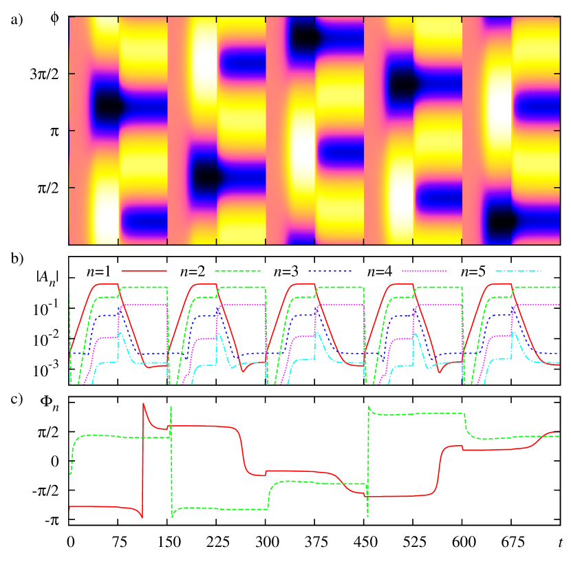
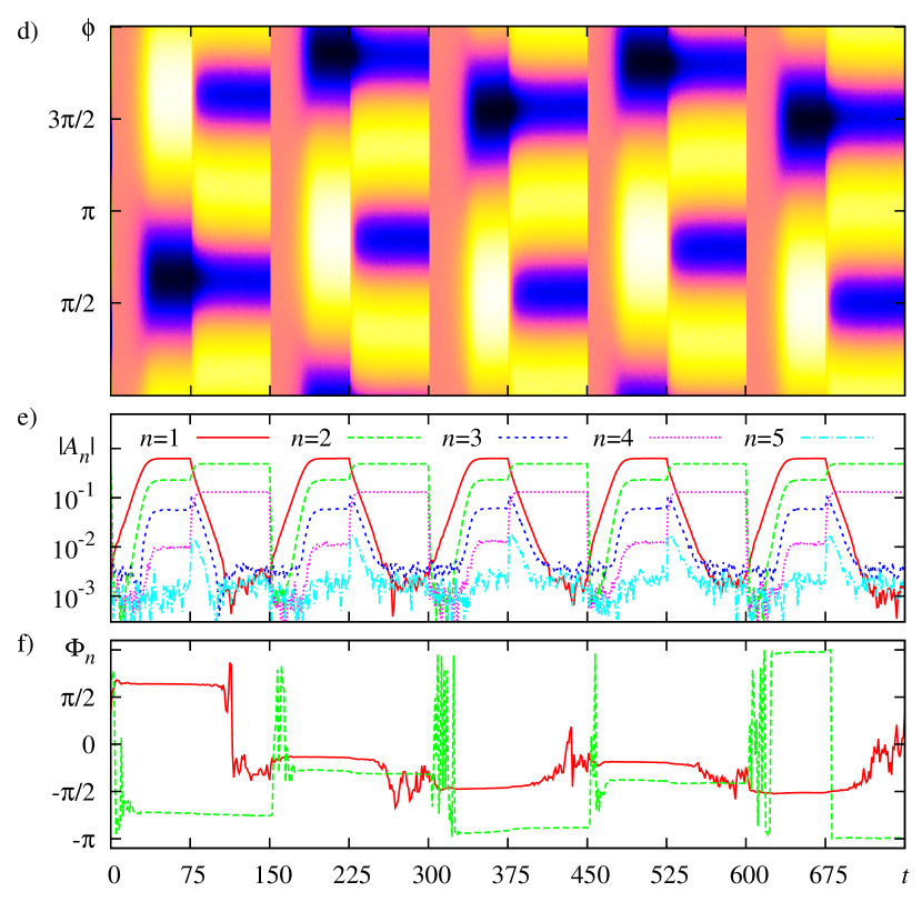
Figure 1: (color online) a) Probability density $v(\phi,t)$ determined by (5), where $A_{n}(t)$ are computed according to Eq. (12); d) distribution for the ensemble of $\phi_{k}$, see Eq. (14), where the total number of the oscillators is $K=10^{6}$. Darker colors correspond to higher values of $v(\phi,t)$. Five periods of switching of $\tilde{\kappa}_{1,2}(t)$ are shown. b) and c) Absolute values and arguments of $A_{n}$ computed according to Eq. (12); e) and f) the same computed via Eq. (3) for the ensemble. $|A_{n}|$ are plotted in logarithmic scale. Parameters: $\kappa_{1}=1.3$, $\kappa_{2}=2.3$, $T=150$, $\epsilon=0.01$, $\sigma=1$, $\ell_{\text{cut}}=10$.

Figure 1(a) illustrates the temporal behavior of the probability density $v(\phi,t)$ computed according to Eq. (5). At the stage 1 ($0\leq t\leq 75$) the $1$-cluster develops. Then, after the switch to the stage 2 at $t=T/2=75$, the density acquires two humps. One part of the $2$-cluster is located just at the site of the former $1$-cluster, and the second one appears shifted by $\pi$. As we already discussed, this situation corresponds to the quadratic relation for the complex amplitudes $A_{2}\sim A_{1}^{2}$ and to the doubling of the argument. At the initial epoch of the next stage 1 at $t\gtrsim 150$, the $2$-cluster disappears, and the $1$-cluster reappears. Notice that the hump emerges now at a site which is different both from that of the previous $2$-cluster, and that of the former $1$-cluster. It is so because of the presence of a small force $f(\phi)$ corresponding to the term proportional to $\epsilon$ in Eqs. (12).

Figures 1(b) and (c) show magnitudes and arguments of $A_{n}$. At stage 1 all the magnitudes $|A_{n}|$ grow and saturate at some level; in this state the main mode $A_{1}$ dominates. At stage 2 the mode $A_{2}$ grows, together with its harmonics, while all odd modes decay.

Let us now focus on the phase dynamics. The phase $\Phi_{2}$ does not change at the transition from stage 1 to stage 2 at $t=75$. At the beginning of stage 2 the phase of the first mode $\Phi_{1}$ is nearly constant while the amplitude of this mode remains relatively large; however at $t\approx 100$ the amplitude drops to level $\sim\epsilon$, and now this mode becomes to be driven by $\epsilon A_{2}^{*}$. Here, the mode $A_{1}$ accepts the phase $-\Phi_{2}$ that can be seen in Fig. 1(c) as a sharp transition around $t\approx 110$. After this event, the phase of the mode $A_{1}$ does not vary significantly. At $t=T=150$ the new stage 1 starts, here the amplitude of the previously active mode $A_{2}$ decays rapidly, but it reappears soon as the second harmonics of the mode 1, accepting its doubled phase $2\Phi_{1}$ (see the jump of $\Phi_{2}$ at $t\approx 155$ followed by the growth of $|A_{2}|$).

Although the dynamics of the phases and the amplitudes observed in Fig. 1(a,b,c) nicely corresponds to the qualitative picture of section II.3, it is important to verify that the phase evolution really follows the Bernoulli-like map (11). In Fig. 2(a) a diagram is shown for the values of argument of the complex variable $A_{1}$ recorded stroboscopically at $t=t_{n}=(n+\frac{9}{20})T$. Indeed, the plot demonstrates the doubling of the phase, as expected. Thus, actually, the phases of the alternately arising clusters evolve according to the expanding circle map that implies the hyperbolic chaos.

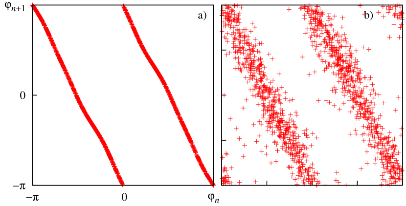
Figure 2: a) The plot $\varphi_{n+1}$ vs. $\varphi_{n}$ where $\varphi_{n}=\arg A_{1}(nT+\frac{9}{20}T)$, and $A_{\ell}$ is a solution of Eqs. (12). b) The same diagram for the ensemble (14), where $A_{1}$ is computed according to Eq. (3). Parameters correspond to Fig. 1.

IV.2 Ensemble of noisy oscillators

Here we report on the results of a straightforward simulation of the ensemble dynamics according to Eqs. (14). We perform numerical solutions for these stochastic differential equations employing a special version of the Runge-Kutta-type algorithm suggested in Honeycutt (1992). Figure 1(d) illustrates the temporal behavior of the probability density $v(\phi,t)$ computed from the instantaneous distributions of the phases $\phi_{k}$ for the elements of the ensemble, and the panels (e) and (f) demonstrate the dynamics of the mean-field variables $A_{n}(t)$. The parameters are the same as in the previous simulations of the Fokker-Plank equation. Except for the obvious difference in the initial conditions, the distributions $v(\phi,t)$ and the magnitudes of $A_{n}(t)$ at their high levels behave visually similar. The dynamics of the phases is definitely more noisy than that in Fig. 1(c), especially in the regions where the magnitudes of the corresponding modes are small: in these regions even small finite-size fluctuations produce a large effect on the phases. When the magnitude of $A_{1}(t)$ is high (see for example the time interval $30<t<75$), its argument does not respond to the noise. But when $A_{1}$ gets small, the argument fluctuates (see the time interval $110<t<150$). The same is true for $A_{2}$. The most harmful are the fluctuations of $\Phi_{1}$ because this variable inherits the argument value from $A_{2}$ when $|A_{1}|$ is small. If the fluctuations are strong enough, they wash out the correct value of the argument, and the phase multiplication mechanism ceases to operate properly. The fluctuations of $A_{2}$ are not so essential since they occur only in epochs, when the component $A_{2}$ does not play an important role. One can see from the figure that the phase transfer happens when $A_{2}$ has a large magnitude and thus is not affected by the noise (see the time interval $180<t<225$).

Figure 2(b) shows the diagram for the stroboscopically recorded values of $\Phi_{1}$ corresponding to the dynamical behavior illustrated in Fig. 1(d,e,f). One can observe that the phases demonstrate the expected Bernoulli-like doubling mapping in average, though the fluctuations produce a noticeable statistical widening (which decreases as the size of the ensemble $K$ grows).

IV.3 Lyapunov exponent and hyperbolicity test

Now we return to the Fokker–Plank system (12) and discuss how the Lyapunov exponents (LEs) depend on $\kappa_{1}$ and $\kappa_{2}$. Also we test hyperbolicity of the chaotic dynamics of the system (12).

We calculate the Lyapunov exponents in the deterministic system (12) with the standard Benettin algorithm. Because the system is periodically driven, we report as LEs the values $\Lambda=\lambda T$, i.e. the “Lyapunov multipliers” over the period. In all cases we have found at most one positive LE, the others were negative. Figure 3(a) shows the largest LE versus parameter $\kappa_{1}$; in a large range of this parameter it is positive and close to the expected value $\ln 2\approx 0.69314$. The other exponents are all negative, and their magnitudes are much higher. For example, at $\kappa_{1}=1.3$, and $\kappa_{2}=2.3$ we have $\Lambda_{i}=\{0.688,-17.355,-197.507,-245.781,-705.748\}$, and the corresponding Kaplan-Yorke dimension is $1.04$.

The positive Lyapunov exponent varies slowly depending on the parameter, but no tips or dips, like in many non-hyperbolic systems, are observed. This may be regarded as a manifestation of the structural stability intrinsic to the hyperbolic dynamics. Figure 4(a) represents dependence of $\Lambda$ on $\kappa_{2}$, while $\kappa_{1}$ is constant. Again, the same features are observed: the largest Lyapunov exponent is close to the value $\ln 2$, and it does not demonstrate any notable variation within a wide range of the parameter.

To test hyperbolicity, we employed the method which has been specially developed for high-dimensional systems, see Ref. Kuptsov (2012) for details and Ref. Kuptsov and Parlitz (2012) for the mathematical background. In brief, the method includes the computation of the first $k$ orthogonalized Lyapunov vectors moving forward in time (so called Gram-Schmidt vectors or backward Lyapunov vectors Kuptsov and Parlitz (2012)), and also the first $k$ orthogonalized Lyapunov vectors obtained moving backward in time from the conjugate variational equations (forward Lyapunov vectors); here $k$ is the dimension of the unstable manifold. Given these vectors, a $k\times k$ matrix of their scalar products is built. Its smallest singular value $d_{k}$ is cosine of the angle between the expanding tangent subspace and the orthogonal complement to the contracting tangent subspace, and thus $d_{k}$ can be an indicator of hyperbolicity. For a non-hyperbolic case, the $d_{k}$ values vanish somewhere along the trajectories (as the tangencies between the associated expanding and contracting subspaces occur), but for situations of the hyperbolic dynamics the distribution of $d_{k}$ is well separated from zero.

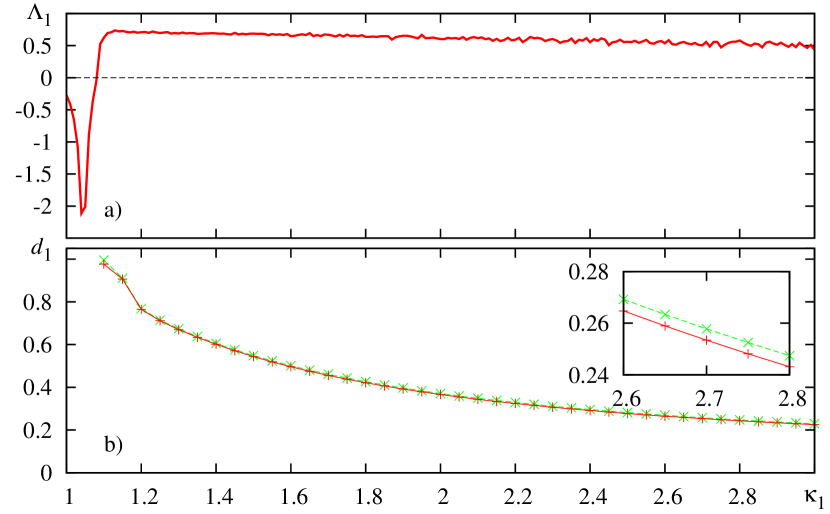
Figure 3: (a) The first Lyapunov exponent, and (b) the lower and upper boundaries of the distribution of $d_{1}$ vs. $\kappa_{1}$. The data relate to the stroboscopic map corresponding to the Fokker-Plank system (12) at $t_{n}=(n+\frac{9}{20})T$ . Distributions of $d_{1}$ for each $\kappa_{1}$ were computed for $10^{4}$ attractor points. $\kappa_{2}=2.3$, other parameters correspond to Fig. 1.

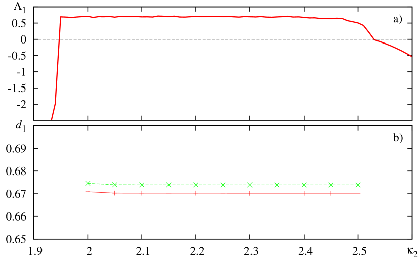
Figure 4: The same quantities as in Fig. 3 against $\kappa_{2}$, while $\kappa_{1}=1.3$.

In Fig. 3(b) we illustrate the results of this hyperbolicity test. In our case the expanding subspace is one-dimensional. Thus, for each $\kappa_{1}$ we compute $10^{4}$ points on the attractor of the stroboscopic map, and evaluate the indicator $d_{1}$ at each of them. Then, the smallest and the largest values of $d_{1}$ are plotted on the diagram, marked with crosses and pluses, respectively. The first observation is that the smallest $d_{1}$ is very far from zero; this confirms the hyperbolicity. Another noteworthy observation is that the maximal and the minimal values of $d_{1}$ are very close to each other. This means that the mutual orientations of the expanding and contracting directions remain practically unaltered on the entire attractor. This can be treated as another manifestation of the structural stability. Figure 4(b) shows the hyperbolicity indicator $d_{1}$ in dependence on $\kappa_{2}$, it is again well separated from zero.

IV.4 Lyapunov exponents for the micro-level dynamics

It is instructive to compare the macroscopic LEs for the dynamics of the order parameters with microscopic LEs describing stability of the dynamics of individual oscillators. A direct approach to computation of the full spectrum of Lyapunov exponents for the ensemble of phase oscillators (14) can easily exhaust a computer memory and take an extremely long time. However, there is a simple way to estimate microscopic LEs assuming their decoupling from the macroscopic dynamics. Neglecting small $\epsilon$ in Eq. (3), we can rewrite this equation as

$$\dot{\phi}_{k}=\frac{1}{2\mathrm{i}}\sum_{n=1}^{2}\tilde{\kappa}_{n}(A_{n}e^{-\mathrm{i}n\phi_{k}}-A_{n}^{*}e^{\mathrm{i}n\phi_{k}})+\sigma\xi_{k}(t)\;.$$ (15)

Let us now assume that on stages 1 and 2 the order parameters $A_{1}$ and $A_{2}$ are roughly constant. Then the variations of the phases satisfy

$$\frac{1}{\delta\phi_{k}}\frac{d}{dt}\delta\phi_{k}=-\sum_{n=1}^{2}n\tilde{\kappa}_{n}(A_{n}e^{-\mathrm{i}n\phi_{k}}+A_{n}^{*}e^{\mathrm{i}n\phi_{k}}).$$ (16)

Now the microscopic LE is evaluated as an average of the r.h.s. of Eq. (16) multiplied by $T/2$, which yields $\Lambda_{\text{mic}}=-\frac{T}{2}\sum_{n=1}^{2}n\tilde{\kappa}_{n}|A_{n}|^{2}$. Substituting here the approximate expressions for stationary magnitudes of the order parameters, valid for small subcritical couplings $\kappa_{1}\gtrsim\sigma^{2}$, $\kappa_{2}\gtrsim 2\sigma^{2}$, we obtain the following estimate:

$$\Lambda_{\text{mic}}\approx-T\sigma^{2}\left(\frac{\kappa_{1}-\sigma^{2}}{\kappa_{1}}+4\frac{\kappa_{2}-2\sigma^{2}}{\kappa_{2}}\right)\;.$$ (17)

For the parameters used above, $\sigma=1,\kappa_{1}=1.3,\kappa_{2}=2.3,T=150$, this yields $\Lambda_{\text{mic}}\approx-113$ in a reasonable agreement with the numerics.

Thus, contrary to many situations where chaos occurs in the micro-level description, while the macro-parameters manifest rather regular behavior, here we observe an impressively opposite case: the micro-dynamics is stable (because $\Lambda_{\text{mic}}<0$), but at the macro-level the hyperbolic chaos takes place.

V Conclusion

In this paper we have demonstrated that blinking coupling in populations of noisy oscillators may result in hyperbolic chaos of macroscopic mean fields. The blinking is between two simplest modes of coupling: one leads to a one-cluster synchronized state, another one leads to appearance of two clusters, shifted by $\pi$. Correspondingly, at these couplings two different order parameters dominate: the usual Kuramoto order parameter for the one-cluster state, and the second-harmonics Daido order parameter for the two-cluster state. While the magnitudes of these order parameters show no significant variations from cycle to cycle, the phases obey a strongly chaotic Bernoulli transformation, and thus demonstrate a hyperbolic chaos. Noteworthy, there is a realistic situation where the two types of global coupling (one-cluster and two-cluster) can be observed: this is an ensemble of pendula hanging on a common beam. In such a configuration with two pendulum clocks Ch. Hyugens observed synchronization more than 300 years ago (see a translation of his notes in Pikovsky et al. (2001)). Nowadays one reproduces these experiments with metronomes Kapitaniak et al. (2012). The horizontal motions of the beam result in the one-cluster coupling, while the vertical motions lead to the two-cluster coupling Czolczyński et al. (2013).

Our analysis is mostly based on the consideration of the thermodynamic limit, where the population can be described by the nonlinear Fokker-Planck equation. We verify hyperbolic chaos in this integral-differential equation, by direct simulations of equations for the modes and showing that their phases obey a Bernoulli map, and by checking that the stable and the unstable directions in the tangent space are never tangent to each other. For the original population a direct simulation gives a picture very similar to that for the nonlinear Fokker-Planck equation, but the one-dimensional transformation of the phases looks like a noisy Bernoulli map, due to finite-size effects.

In a more general perspective, the nonlinear Fokker-Planck equation, as an integro-differential equation with partial derivatives, is a representative of a class of deterministic distributed systems demonstrating pattern formation. Different cluster synchronization states correspond to different patterns; phases of clusters correspond to the spatial positions of the patterns. With this interpretation, our results demonstrate that an interaction between blinking patterns results in a chaotic relocation of their positions, moreover, this chaos is hyperbolic. A kind of such behavior was reported recently in a model of interacting Turing patterns with different wave numbers Kuptsov et al. (2012). The presented model based on the nonlinear Fokker–Plank equation provides another indication that the above mechanism of the hyperbolic chaos is realizable in quite generic circumstances.

The authors acknowledge support from the RFBR grant No 11-02-91334 and DFG grant No PI 220/14-1.

References

- Kuramoto (1984) Y. Kuramoto, Chemical Oscillations, Waves and Turbulence (Springer, Berlin, 1984).
- Pikovsky et al. (2001) A. Pikovsky, M. Rosenblum, and J. Kurths, Synchronization. A Universal Concept in Nonlinear Sciences. (Cambridge University Press, Cambridge, 2001).
- Ott and Antonsen (2008) E. Ott and Th. M. Antonsen, “Low dimensional behavior of large systems of globally coupled oscillators,” CHAOS 18, 037113 (2008).
- Kaneko (1992) K. Kaneko, “Mean field fluctuation of a network of chaotic elements,” Physica D 55, 368 (1992).
- Pikovsky and Kurths (1994) A. S. Pikovsky and J. Kurths, “Collective behavior in ensembles of globally coupled maps,” Physica D 76, 411–419 (1994).
- Pikovsky et al. (1996) A. Pikovsky, M. Rosenblum, and J. Kurths, “Synchronization in a population of globally coupled chaotic oscillators,” Europhys. Lett. 34, 165–170 (1996).
- Topaj et al. (2001) D. Topaj, W.-H. Kye, and A. Pikovsky, “Transition to coherence in populations of coupled chaotic oscillators: A linear response approach,” Phys. Rev. Lett. 87, 074101 (2001).
- Ott et al. (2002) E. Ott, P. So, E. Barreto, and T. Antonsen, “The onset of synchronization in systems of globally coupled chaotic and periodic oscillators,” Physica D 173, 29–51 (2002).
- Hakim and Rappel (1992) V. Hakim and W. J. Rappel, “Dynamics of the globally coupled complex Ginzburg-Landau equation,” Phys. Rev. A 46, R7347–R7350 (1992).
- Nakagawa and Kuramoto (1994) N. Nakagawa and Y. Kuramoto, “From collective oscillations to collective chaos in a globally coupled oscillator system,” Physica D 75, 74–80 (1994).
- Kuznetsov et al. (2010) S. P. Kuznetsov, A. Pikovsky, and M. Rosenblum, “Collective phase chaos in the dynamics of interacting oscillator ensembles,” CHAOS 20 (2010), 10.1063/1.3527064.
- Desai and Zwanzig (1978) R. C. Desai and R. Zwanzig, “Statistical mechanics of a nonlinear stochastic model,” J. Stat. Phys. 19, 1 (1978).
- Dawson (1983) D. A. Dawson, “Critical dynamics and fluctuations for a mean–field model of cooperative behaviour,” J. Stat. Phys. 31, 29 (1983).
- Bonilla et al. (1992) L. L. Bonilla, J. C. Neu, and R. Spigler, “Nonlinear stability of incoherence and collective synchronization in a population of coupled oscillators,” J. Stat. Phys. 67, 313–330 (1992).
- Pikovsky and Ruffo (1999) A. Pikovsky and S. Ruffo, “Finite-size effects in a population of interacting oscillators,” Phys. Rev. E 59, 1633–1636 (1999).
- Belykh et al. (2004) Igor V. Belykh, Vladimir N. Belykh, and Martin Hasler, “Blinking model and synchronization in small-world networks with a time-varying coupling,” Physica D: Nonlinear Phenomena 195, 188 – 206 (2004).
- Wang et al. (2010) Lei Wang, Huan Shi, and You-xian Sun, “Induced synchronization of a mobile agent network by phase locking,” Phys. Rev. E 82, 046222 (2010).
- Porfiri (2012) Maurizio Porfiri, “Stochastic synchronization in blinking networks of chaotic maps,” Phys. Rev. E 85, 056114 (2012).
- Kuznetsov (2012) S. P. Kuznetsov, Hyperbolic Chaos: A Physicist’s View (Higher Education Press: Bijing and Springer-Verlag: Berlin, Heidelberg, 2012) p. 336.
- Kuznetsov (2011) S. P. Kuznetsov, “Dynamical chaos and uniformly hyperbolic attractors: from mathematics to physics,” Physics-Uspekhi 54, 119–144 (2011).
- Smale (1967) S. Smale, “Differentiable dynamical systems,” Bull. Am. Math. Soc. 73, 747–817 (1967).
- Kuznetsov (2005) S. P. Kuznetsov, “Example of a physical system with a hyperbolic attractor of the Smale-Williams type,” Phys. Rev Lett. 95, 144101 (2005).
- Kuznetsov and Pikovsky (2007) S. P. Kuznetsov and A. Pikovsky, “Autonomous coupled oscillators with hyperbolic strange attractors,” Physica D 232, 87–102 (2007).
- Kuptsov et al. (2012) P. V. Kuptsov, S. P. Kuznetsov, and A. Pikovsky, “Hyperbolic chaos of Turing patterns,” Phys. Rev. Lett. 108, 194101 (2012).
- Cox and Matthews (2002) S.M. Cox and P.C. Matthews, “Exponential time differencing for stiff systems,” Journal of Computational Physics 176, 430 – 455 (2002).
- Honeycutt (1992) R. L. Honeycutt, “Stochastic Runge-Kutta algorithms. I. White noise,” Phys. Rev. A 45, 600–603 (1992).
- Kuptsov (2012) P. V. Kuptsov, “Fast numerical test of hyperbolic chaos,” Phys. Rev. E 85, 015203 (2012).
- Kuptsov and Parlitz (2012) P. Kuptsov and U. Parlitz, “Theory and computation of covariant Lyapunov vectors,” Journal of Nonlinear Science 22, 727–762 (2012).
- Kapitaniak et al. (2012) M. Kapitaniak, K. Czolczyński, P. Perlikowski, A. Stefański, and T. Kapitaniak, “Synchronization of clocks,” Physics Reports 517, 1–69 (2012).
- Czolczyński et al. (2013) K. Czolczyński, P. Perlikowski, A. Stefański, and T. Kapitaniak, “Synchronization of the self-excited pendula suspended on the vertically displacing beam,” Communications in Nonlinear Science and Numerical Simulation 18, 386 – 400 (2013).