On the Damping-Induced Self-Recovery Phenomenon in
Mechanical Systems with
Several Unactuated Cyclic Variables

Abstract

The damping-induced self-recovery phenomenon refers to the fundamental property of underactuated mechanical systems: if an unactuated cyclic variable is under a viscous damping-like force and the system starts from rest, then the cyclic variable will always move back to its initial condition as the actuated variables come to stop. The regular momentum conservation phenomenon can be viewed as the limit of the damping-induced self-recovery phenomenon in the sense that the self-recovery phenomenon disappears as the damping goes to zero. This paper generalizes the past result on damping-induced self-recovery for the case of a single unactuated cyclic variable to the case of multiple unactuated cyclic variables. We characterize a class of external forces that induce new conserved quantities, which we call the damping-induced momenta. The damping-induced momenta yield first-order asymptotically stable dynamics for the unactuated cyclic variables under some conditions, thereby inducing the self-recovery phenomenon. It is also shown that the viscous damping-like forces impose bounds on the range of trajectories of the unactuated cyclic variables. Two examples are presented to demonstrate the analytical discoveries: the planar pendulum with gimbal actuators and the three-link planar manipulator on a horizontal plane.

Keywords: Mechanical system, cyclic variable, viscous damping, self-recovery

1 Introduction

Mechanical systems of kinematically coupled structures, or multibody systems, have a variety of engineering applications including robotic manipulators, manufacturing machines with articulated components, bipedal walking and musculoskeletal system modeling [5]. An interesting aspect of such systems is how they behave when certain degrees of freedom are left unactuated. In dealing with such underactuated mechanical systems, we often explore their fundamental properties. For instance, if the unactuated variables are cyclic (i.e. do not appear in the Lagrangian), then the momentum map associated with these variables will be conserved due to symmetry [7]. One of the most celebrated examples of the symmetry and conservation of momentum is the falling cat problem [4, 8, 9]: a cat always lands on its feet after released upside down from rest, by deforming its body while keeping a zero angular momentum. There are variants of the falling cat such as Elroy’s beanie [6] and springboard divers [2]. Another popular example is the system of a human sitting on a rotating stool holding a wheel [1]. Sitting on the rotating stool, one spins the wheel by his hand while holding it horizontally. A reaction torque will be created and initiate the rotating motion of the stool in the opposite direction. As long as the wheel is rotating, the stool keeps rotating. After some time, if the person applies a braking force halting the wheel spin, then the stool will also stop. All of these phenomena follow from angular momentum conservation, which holds in the absence of external forces. If there is an external force, then the momentum is not conserved any longer in general and the consequent motion of the system will be different from that in the case of momentum conservation.

We are here mainly interested in the case where the external forces are linear in the velocity, i.e. viscous damping-like forces. This was well studied in [1] for the case of one-dimensional symmetry, i.e., $S^{1}$ or $\mathbb{R}^{1}$ symmetry. According to [1], in the stool-wheel system with viscous damping friction on the rotation axis of the stool, the stool does not keep rotating but meets a bound in its motion even if the person on the stool keeps spinning the wheel. The larger the angular velocity of the spin of the wheel is, the more angle the stool rotates by, but in the end the stool meets a bound in its motion, not being able to keep rotating, as long as the angular velocity of the wheel is bounded. This bound on the motion of the stool is called the damping-induced bound. Another phenomenon, which is perhaps more remarkable, in this stool-wheel system with the friction is the following. After some time, if the person on the stool stops the spinning of the wheel, then the stool does not stop. Instead, it asymptotically converges back to its initial position, making the same number of net rotations in the opposite direction. This phenomenon is called damping-induced self-recovery. From this example, one can see that the viscous damping-like force plays a role of a restoring force, but it is different from the spring force. To the knowledge of the authors, an example of damping-induced self-recovery and boundedness was first reported by Andy Ruina at a conference [10], where he shows a video of his experiment and provides an intuitive proof of the phenomena. The damping-induced self-recovery phenomenon, without damping-induced boundedness, is also explained in [3] for the case where the damping coefficient is constant, but the proof therein is not complete. Both phenomena of damping-induced self-recovery and damping-induced boundedness were rigorously and completely proved for the first time in [1], where the damping coefficient is allowed to be a function of the cyclic variable and may take some negative values. The results in [1] as well as [10, 3] are for the case of one-dimensional symmetry.

This paper generalizes the results in [1] to the case of higher-dimensional Abelian symmetry. We consider mechanical systems with several unactuated cyclic variables that are subject to external forces linear in the velocity. The systems are allowed to have some actuated variables that are subject to control forces. We find conditions on the linear forces under which the damping-induced phenomena of self-recovery and boundedness occur for the cyclic variables. The analytical approach taken in this paper for the proof of these two phenomena is different from that in [1]. The total order of $\mathbb{R}$ was implicitly made use of in [1], but in this paper we employ a Lyapunov-like function to prove the damping-induced self-recovery and boundedness for the multiple cyclic variables. We first characterize a class of damping-like forces that induce new conserved quantities which we call in this paper the damping-added momenta, and then construct a Lyapunov-like function using the damping-added momenta to prove the existence of the phenomena of damping-induced self-recovery and boundedness. To illustrate the main results, we consider two nontrivial examples of multibody systems that possess multiple cyclic variables: the planar pendulum with gimbal actuators and the three-link planar manipulator on a horizontal plane.

2 Main Results

In this paper, the norm $\|\cdot\|$ denotes the Euclidean norm for vectors and the corresponding induced norm for matrices. For an invertible matrix $A=(a_{ij})$, the $(i,j)$-th entry of its inverse matrix is denoted by $a^{ij}$. For a symmetric matrix $A$ we denote its positive semi-definiteness by $A\succeq 0$. For two symmetric matrices $A$ and $B$ of the same size, $A\succeq B$ means $A-B\succeq 0$.

2.1 Equations of Motion and Damping-Added Momenta

Let $Q=Q_{1}\times Q_{2}$ be an $n$-dimensional configuration space, where $Q_{1}=\mathbb{R}^{r}$ and $Q_{2}$ is a smooth manifold of dimension $n-r$. If a unit circle $S^{1}$ appears as a factor of $Q_{1}$, it is replaced by $\mathbb{R}$, which does not impose any restrictions on the description of the dynamics. Let $q=(x,y)\in\mathbb{R}^{r}\times Q_{2}$ denote coordinates for $Q$, where

$$x=(x^{\alpha})=(x^{1},\ldots,x^{r}),\quad y=(y^{a})=(y^{r+1},\ldots,y^{n})$$

and

$$q=(q^{i})=(q^{1},\ldots,q^{r};q^{r+1},\ldots,q^{n})=(x^{1},\ldots,x^{r};y^{r+1},\ldots,y^{n}).$$

For notational convenience, the following three groups of indices are used in this paper:

$$\underbrace{\underbrace{1,\ldots,r}_{\alpha,\beta,\gamma,\ldots};\underbrace{r+1,\ldots,n}_{a,b,c,\ldots}}_{i,j,k...}.$$

Consider a mechanical system with the Lagrangian

$$L(q,\dot{q})=\frac{1}{2}m_{\alpha\beta}\dot{x}^{\alpha}\dot{x}^{\beta}+m_{\alpha a}\dot{x}^{\alpha}\dot{y}^{a}+\frac{1}{2}m_{ab}\dot{y}^{a}\dot{y}^{b}-V(q)$$

which is the kinetic minus potential energy of the system. Here we follow the Einstein summation convention. It is assumed that the mass matrix

$$m=\begin{pmatrix}m_{\alpha\beta}&m_{\alpha b}\\ m_{a\beta}&m_{ab}\end{pmatrix}$$

is symmetric and positive definite.

We make the following four assumptions on the system:

• The variables $x^{\alpha}$’s are cyclic [7], i.e.

  $$\frac{\partial L}{\partial x^{\alpha}}=0$$

  for all $\alpha=1,\ldots,r$.

• Controls $u_{a}$’s are given in the directions of $y^{a}$’s.

• Each cyclic variable $x^{\alpha}$ is under a general damping-like force (i.e. linear in the velocity) described as $-k_{\alpha\beta}(x)\dot{x}^{\beta}$, where each coefficient $k_{\alpha\beta}(x)$ is a continuously differentiable function of $x$.

• The coefficients $k_{\alpha\beta}$ satisfy

  $$k_{\alpha\beta}=k_{\beta\alpha}$$ (1)

  and

  $$\frac{\partial k_{\alpha\beta}}{\partial x^{\gamma}}=\frac{\partial k_{\alpha\gamma}}{\partial x^{\beta}}.$$ (2)

By A1) – A3), the equations of motion of the system are written as

$$\frac{d}{dt}\frac{\partial L}{\partial\dot{x}^{\alpha}} =-k_{\alpha\beta}\dot{x}^{\beta},\quad\alpha=1,\ldots,r$$ (3)

$$\frac{d}{dt}\frac{\partial L}{\partial\dot{y}^{a}}-\frac{\partial L}{\partial y^{a}} =u_{a},\quad a=r+1,\ldots,n.$$ (4)

In individual coordinates, (3) and (4) can be expressed as

$$m_{\alpha\beta}\ddot{x}^{\beta}+m_{\alpha b}\ddot{y}^{b}+[ij,\alpha]\dot{q}^{i}\dot{q}^{j}=-k_{\alpha\beta}\dot{x}^{\beta}$$ (5)

$$m_{a\beta}\ddot{x}^{\beta}+m_{ab}\ddot{y}^{b}+[ij,a]\dot{q}^{i}\dot{q}^{j}+\frac{\partial V}{\partial y^{a}}=u_{a},$$ (6)

where $[ij,k]$ denotes the Christoffel symbol

$$[ij,k]=\frac{1}{2}\left(\frac{\partial m_{ik}}{\partial q^{j}}+\frac{\partial m_{jk}}{\partial q^{i}}-\frac{\partial m_{ij}}{\partial q^{k}}\right)$$

for $i,j,k=1,\ldots,n$.

If there were no external forces, i.e. $k_{\alpha\beta}=0$ for all $\alpha,\beta$, then the momenta $\frac{\partial L}{\partial\dot{x}^{\alpha}}$’s would be the first integrals of the system (3), but due to the external forces $F_{\alpha}=-k_{\alpha\beta}\dot{x}^{\beta}$’s, $\frac{\partial L}{\partial\dot{x}^{\alpha}}$’s are not conserved any more. We will here show that there are new conserved quantities associated with (3) in place of $\frac{\partial L}{\partial\dot{x}^{\alpha}}$’s.

Lemma 2.1.

Assumption A4) entails the following:

1. For each $\alpha$, there is a function $h_{\alpha}:\mathbb{R}^{r}\rightarrow\mathbb{R}$ such that

   $$\frac{\partial h_{\alpha}}{\partial x^{\beta}}=k_{\alpha\beta}.$$ (7)

2. For each $h_{\alpha}$, there is a function $U:\mathbb{R}^{r}\rightarrow\mathbb{R}$ such that

   $$\frac{\partial U}{\partial x^{\alpha}}=h_{\alpha}.$$ (8)

   Namely, the damping coefficient matrix ($k_{\alpha\beta}(x)$) is the second-order derivative matrix of $U$.

Proof.

1. By (2) and Ponicaré’s lemma, there is a function $h_{\alpha}$ that satisfies (7).

2. By (1) and (7), we have ${\partial h_{\alpha}}/{\partial x^{\beta}}=k_{\alpha\beta}=k_{\beta\alpha}={\partial h_{\beta}}/{\partial x^{\alpha}}$. Hence, by Ponicaré’s lemma, there is a function $U:\mathbb{R}^{r}\rightarrow\mathbb{R}$ such that (8) holds.

∎

Using Lemma 2.1, we now show that the dynamics (3) have $r$ first integrals.

Theorem 2.2.

Let $h_{\alpha}$’s be functions that satisfy (7). Then, the $r$ functions

$$\frac{\partial L}{\partial\dot{x}^{\alpha}}+h_{\alpha}$$ (9)

or equivalently

$$m_{\alpha\beta}\dot{x}^{\beta}+m_{\alpha a}\dot{y}^{a}+h_{\alpha}$$ (10)

for $\alpha=1,\ldots,r,$ are the first integrals of the dynamics (3).

Proof.

Differentiating (9) with respect to $t$ along the trajectory of the system gives

$$\frac{d}{dt}\left(\frac{\partial L}{\partial\dot{x}^{\alpha}}+h_{\alpha}\right)=\frac{d}{dt}\frac{\partial L}{\partial\dot{x}^{\alpha}}+\frac{\partial h_{\alpha}}{\partial x^{\beta}}\dot{x}^{\beta}=-k_{\alpha\beta}\dot{x}^{\beta}+k_{\alpha\beta}\dot{x}^{\beta}=0$$

due to (3) and (7). This completes the proof. ∎

The vector-valued map $(q,\dot{q})\mapsto(\frac{\partial L}{\partial\dot{x}^{\alpha}}+h_{\alpha})$ shall be called the damping-added momentum map.

2.2 Damping-Induced Self-Recovery and Damping-Induced Boundedness

The first integrals in (9) depend on the initial condition $(x(0),y(0),\dot{x}(0),\dot{y}(0))$. Taking an arbitrary initial condition and letting $\mu_{\alpha}$ be the initial value of the corresponding first integral, $\frac{\partial L}{\partial\dot{x}^{\alpha}}+h_{\alpha}$, we have

$$m_{\alpha\beta}\dot{x}^{\beta}+m_{\alpha a}\dot{y}^{a}+h_{\alpha}(x)=\mu_{\alpha}$$ (11)

for all $t\in\mathbb{R}$. By Lemma 2.1, there is a function $U$ on $\mathbb{R}^{r}$ such that (8) holds. By adding $-\mu_{\alpha}x^{\alpha}$ to it, we can obtain a function $U_{\mu}:\mathbb{R}^{r}\rightarrow\mathbb{R}$ such that

$$\frac{\partial U_{\mu}(x)}{\partial x^{\alpha}}=h_{\alpha}(x)-\mu_{\alpha}.$$ (12)

The conservation equations (11) for the damping-added momenta can be regarded as first-order differential equations for the cyclic variables $x^{\alpha}$’s. The damping-induced self-recovery phenomenon is a direct consequence of asymptotic stability of these first-order dynamics under some conditions on the function $U_{\mu}$. Let us make the following assumptions on $U_{\mu}$ which constitute sufficient conditions for the self-recovery phenomenon to occur:

• The function $U_{\mu}$ has a unique critical point, denoted $x_{e}$, and it is a minimum point of $U_{\mu}$.

• There is a number $\delta_{1}>0$ such that

  $$\inf_{\|x-x_{e}\|\geq\delta_{1}}U_{\mu}(x)>U_{\mu}(x_{e}).$$

• There is a number $\delta_{2}>0$ such that

  $$\inf_{\|x-x_{e}\|\geq\delta_{2}}\|dU_{\mu}(x)\|>0,$$

  where $dU_{\mu}=(\frac{\partial U_{\mu}}{\partial x^{1}},\ldots,\frac{\partial U_{\mu}}{\partial x^{r}})$.

Assumption A6) guarantees that there does not exist any sequence $\{x_{k}\}$ in $\mathbb{R}^{r}$ with $\lim_{k\rightarrow\infty}\|x_{k}\|=\infty$ such that $\lim_{k\rightarrow\infty}U_{\mu}(x_{k})=U_{\mu}(x_{e})$. Likewise, assumption A7) guarantees that there does not exist any sequence $\{x_{k}\}$ in $\mathbb{R}^{r}$ with $\lim_{k\rightarrow\infty}\|x_{k}\|=\infty$ such that $\lim_{k\rightarrow\infty}\|dU_{\mu}(x_{k})\|=0$.

We now state one of the two main theorems of this paper.

Theorem 2.3 (Damping-Induced Self-Recovery).

Suppose that controls $u_{a}(t)$’s are chosen such that $\lim_{t\rightarrow\infty}\dot{y}(t)=0$ and there are numbers $c_{1}>0$, $c_{2}>0$ and $c_{3}>0$ such that

$$c_{1}I\preceq(m_{\alpha\beta}(y(t)))\preceq c_{2}I$$ (13)

$$\|(m_{\alpha a}(y(t)))\|\leq c_{3}$$ (14)

for all $t\geq 0$. Then, $\lim_{t\rightarrow\infty}x(t)=x_{e}$ and $\lim_{t\rightarrow\infty}\dot{x}(t)=0$. In particular, if the initial condition is such that $\dot{x}(0)=0$ and $\dot{y}(0)=0$, then $\lim_{t\rightarrow\infty}x(t)=x(0)$.

Proof.

By (7), integration of (3) with respect to $t$ yields (11) for some constants $\mu_{\alpha}$’s, which can be written as

$$\dot{x}^{\alpha}=-m^{\alpha\beta}\frac{\partial U_{\mu}}{\partial x^{\beta}}-m^{\alpha\beta}m_{\beta a}\dot{y}^{a}$$ (15)

by (12). By adding a constant, we may assume that $U_{\mu}(x_{e})=0$. For each $s>0$, define an open set $W_{s}$ in $\mathbb{R}^{r}$ by

$$W_{s}=\{x\in\mathbb{R}^{r}\mid U_{\mu}(x)<s\}.$$

Take any $\epsilon>0$. We will find a number $T>0$ such that $\|x(t)-x_{e}\|<\epsilon$ for all $t\geq T$.

By A5) and A6), there is a sufficiently small $\delta>0$ such that

$$x\in W_{\delta}\Rightarrow\|x-x_{e}\|<\epsilon.$$ (16)

Replacing $\delta$ by a smaller positive number if necessary, we can find, by A5) – A7), an $\epsilon_{1}>0$ such that

$$x\notin W_{\delta}\Rightarrow\|dU_{\mu}(x)\|\geq\epsilon_{1}.$$ (17)

Since the matrix $(m_{\alpha\beta})$ is symmetric and positive definite, (13) implies

$$\frac{1}{c_{2}}I\preceq(m^{\alpha\beta}(y(t)))\preceq\frac{1}{c_{1}}I.$$ (18)

Choose a number $0<\ell<1$ such that

$$\frac{1}{c_{2}}\left(1-\frac{1}{2}\ell\right)^{2}-\frac{1}{4c_{1}}\ell^{2}>0,$$ (19)

which is always possible since the left hand side of (19) is continuous in $\ell$ and is positive at $\ell=0$. Since $\lim_{t\rightarrow\infty}\dot{y}(t)=0$ and the matrix $(m_{\alpha a}(y(t)))$ is bounded, there is a $T_{1}>0$ such that

$$\|(m_{\alpha a}(y(t))\dot{y}^{a}(t))\|<\ell\epsilon_{1}$$ (20)

for all $t\geq T_{1}$. Whenever $x(t)\notin W_{\delta}$ for some $t\geq T_{1}$, we have, by (15), (17), (18) and (20),

$$\frac{dU_{\mu}(x(t))}{dt} =\frac{\partial U_{\mu}(x)}{\partial x^{\alpha}}\dot{x}^{\alpha}$$

$$=\frac{\partial U_{\mu}}{\partial x^{\alpha}}\left(-m^{\alpha\beta}\frac{\partial U_{\mu}}{\partial x^{\beta}}-m^{\alpha\beta}m_{\beta a}\dot{y}^{a}\right)$$

$$=-m^{\alpha\beta}\left(\frac{\partial U_{\mu}}{\partial x^{\alpha}}+\frac{1}{2}m_{\alpha a}\dot{y}^{a}\right)\left(\frac{\partial U_{\mu}}{\partial x^{\beta}}+\frac{1}{2}m_{\beta b}\dot{y}^{b}\right)+\frac{1}{4}m^{\alpha\beta}m_{\alpha a}\dot{y}^{a}m_{\beta b}\dot{y}^{b}$$

$$\leq-\frac{1}{c_{2}}\left\|\left(\frac{\partial U_{\mu}}{\partial x^{\alpha}}+\frac{1}{2}m_{\alpha a}\dot{y}^{a}\right)\right\|^{2}+\frac{1}{4c_{1}}\|(m_{\alpha a}\dot{y}^{a})\|^{2}$$

$$\leq-\frac{1}{c_{2}}\left|\left\|dU_{\mu}\right\|-\frac{1}{2}\|(m_{\alpha a}\dot{y}^{a})\|\right|^{2}+\frac{1}{4c_{1}}\ell^{2}\epsilon_{1}^{2}$$

$$\leq-\frac{1}{c_{2}}\left|\epsilon_{1}-\frac{1}{2}\ell\epsilon_{1}\right|^{2}+\frac{1}{4c_{1}}\ell^{2}\epsilon_{1}^{2}$$

$$=-\left(\frac{1}{c_{2}}\left(1-\frac{1}{2}\ell\right)^{2}-\frac{1}{4c_{1}}\ell^{2}\right)\epsilon_{1}^{2},$$ (21)

where the right-hand side of (21) is negative by (19). Hence, $U_{\mu}(t)$ decreases at least linearly in time as long as $x(t)\notin W_{\delta}$. By definition of $W_{\delta}$, there must exist $T>T_{1}$ such that $x(t)\in W_{\delta}$ for all $t\geq T$. Thus, $\|x(t)-x_{e}\|<\epsilon$ for all $t\geq T$ by (16). Therefore, $\lim_{t\rightarrow\infty}x(t)=x_{e}$. By taking the limit of both sides of (15), we obtain $\lim_{t\rightarrow\infty}\dot{x}(t)=0$ since $dU_{\mu}(x_{e})=0$ by A5). In particular, if $\dot{x}(0)=0$ and $\dot{y}(0)=0$, then $x_{e}=x(0)$ by A5) and (15), so $\lim_{t\rightarrow\infty}x(t)=x(0)$. ∎

Remark 2.4.

The result in Theorem 2.3 is global. In order to get a local result, one has only to assume A5) – A7) in a neighborhood of $x_{e}$ and to assume that the trajectory $x(t)$ stays in the neighborhood.

As was discovered in the case with a single cyclic variable [1], the viscous damping force not only induces self-recovery but also imposes a bound to the range of the cyclic variable. Such a boundedness property also holds for multiple cyclic variables as stated in the following theorem.

Theorem 2.5 (Damping-Induced Boundedness).

Suppose that the function $U_{\mu}$ satisfies

$$\lim_{\|x\|\rightarrow\infty}\|dU_{\mu}(x)\|=\infty$$ (22)

and

$$\lim_{\|x\|\rightarrow\infty}U_{\mu}(x)=\infty.$$ (23)

If controls $u_{a}(t)$’s are chosen such that $\dot{y}(t)$ is bounded and there exist $c_{1}>0$, $c_{2}>0$ and $c_{3}>0$ such that (13) and (14) hold for all $t\geq 0$, then $x(t)$ is bounded.

Proof.

Since $\dot{y}(t)$ is bounded by assumption, there is a number $c_{4}>0$ such that $\|\dot{y}(t)\|\leq c_{4}$ for all $t\geq 0$. By (22), there is a number $\ell>0$ such that

$$\|x-x_{e}\|\geq\ell\Rightarrow\|dU_{\mu}(x)\|\geq 1+\frac{c_{2}c_{3}c_{4}}{c_{1}}.$$

Suppose that $x(t)$ is not bounded. Then, there are numbers $0<t_{1}<t_{2}$ such that $\|x(t)-x_{e}\|\geq\ell$ for all $t\in[t_{1},t_{2}]$ and $U_{\mu}(x(t_{1}))<U_{\mu}(x(t_{2}))$ by (23). Then, for all $t\in[t_{1},t_{2}]$

$$\frac{dU_{\mu}(t)}{dt} =\frac{\partial U_{\mu}}{\partial x^{\alpha}}\left(-m^{\alpha\beta}\frac{\partial U_{\mu}}{\partial x^{\beta}}-m^{\alpha\beta}m_{\beta a}\dot{y}^{a}\right)$$

$$\leq-\frac{1}{c_{2}}\|dU_{\mu}(x(t))\|^{2}+\frac{c_{3}c_{4}}{c_{1}}\|dU_{\mu}(x(t))\|$$

$$=\left(-\frac{1}{c_{2}}\|dU_{\mu}(x(t))\|+\frac{c_{3}c_{4}}{c_{1}}\right)\|dU_{\mu}(x(t))\|$$

$$\leq\left(-\frac{1}{c_{2}}\left(1+\frac{c_{2}c_{3}c_{4}}{c_{1}}\right)+\frac{c_{3}c_{4}}{c_{1}}\right)\|dU_{\mu}(x(t))\|$$

$$\leq-\frac{1}{c_{2}}.$$

Hence,

$$0<U_{\mu}(x(t_{2}))-U_{\mu}(x(t_{1}))=\int_{t_{1}}^{t_{2}}\frac{dU_{\mu}}{dt}(t)dt\leq-\frac{1}{c_{2}}(t_{2}-t_{1})<0,$$

which is a contradiction. Therefore, $x(t)$ is bounded. ∎

2.3 Diagonal Damping Force: A Special Case

Suppose that there are continuous functions $k_{1},\ldots,k_{r}:\mathbb{R}\rightarrow\mathbb{R}$ such that the damping coefficients $k_{\alpha\beta}$ are given as

$$k_{11}(x)=k_{1}(x^{1});\quad k_{22}(x)=k_{2}(x^{2});\quad\cdots\quad;\quad k_{rr}(x)=k_{r}(x^{r});$$ (24)

$$k_{\alpha\beta}(x)=0\quad\textup{ for $\alpha\neq\beta$}.$$

Notice that we do not assume that $k_{\alpha}(x^{\alpha})$’s take only non-negative values though we call them damping coefficients for convenience.

A function $h_{\alpha}$ satisfying (7) is given by

$$h_{\alpha}(x^{\alpha})=\int_{0}^{x^{\alpha}}k_{\alpha}(s)ds,$$ (25)

where there is no summation over the index $\alpha$. Given $\mu=(\mu_{1},\ldots,\mu_{r})\in\mathbb{R}^{r}$, the function $U_{\mu}$ defined by

$$U_{\mu}(x)=\sum_{\alpha=1}^{r}\int_{0}^{x^{\alpha}}(h_{\alpha}(s)-\mu_{\alpha})ds$$ (26)

satisfies (12).

Corollary 2.6 (Damping-Induced Self-Recovery).

Suppose that the functions $k_{\alpha}$’s given in (24) and the functions $h_{\alpha}$’s defined in (25) satisfy the following:

• For each $\alpha$, the equation $h_{\alpha}(s)-\mu_{\alpha}=0$ has a unique root, which is denoted by $x_{e}^{\alpha}$.

• For each $\alpha$, $k_{\alpha}(x^{\alpha}_{e})>0$.

• For each $\alpha$, there is an open interval $I$ containing $x_{e}^{\alpha}$ such that

  $$\inf_{s\in\mathbb{R}\backslash I}|h_{\alpha}(s)-\mu_{\alpha}|>0.$$

Then, the function $U_{\mu}$ defined in (26) satisfies A5) – A7) such that the conclusions in Theorem 2.3 hold true.

Proof.

Take any $\alpha$ between $1$ and $r$. Since $h^{\prime}_{\alpha}(x_{e}^{\alpha})=k_{\alpha}(x_{e}^{\alpha})>0$, the function $h_{\alpha}(s)-\mu_{\alpha}$ is increasing over an open interval containing $x_{e}^{\alpha}$. Thus, by condition (i), we have $h_{\alpha}(s)-\mu_{\alpha}>0$ for all $s>x_{e}^{\alpha}$ and $h_{\alpha}(s)-\mu_{\alpha}<0$ for all $s<x_{e}^{\alpha}$. It is now straightforward to show that the function $U_{\mu}$ defined in (26) satisfies A5) – A7). ∎

Corollary 2.7 (Damping-Induced Boundedness).

Suppose that the functions $h_{\alpha}$ defined in (25) satisfy the three conidtions in Corollary 2.6 and the following condition:

• For each $\alpha$, $\lim_{s\rightarrow\infty}h_{\alpha}(s)=\infty$ and $\lim_{s\rightarrow-\infty}h_{\alpha}(s)=-\infty$.

Then, the conclusion in Theorem 2.5 holds true.

Proof.

It is easy to show that $U_{\mu}$ given in (26) satisfies (22) and (23). ∎

2.4 Choice of Control for Damping-Induced Self-Recovery

In Theorems 2.3 and 2.5 we have assumed that an appropriate control law exists to satisfy some conditions on the trajectory $y(t)$. We now constructively show that such a control law exists.

Lemma 2.8 ([11]).

The control law

$$u_{a}=f_{a}(y,\dot{x},\dot{y})+g_{ab}(y)\tau^{b},$$ (27)

where $\tau^{b}$’s are new control variables and

$$f_{a} =\left([ij,a]-m_{a\alpha}[ij,\beta]m^{\alpha\beta}\right)\dot{q}^{i}\dot{q}^{j}-m_{a\alpha}m^{\alpha\beta}k_{\beta\gamma}\dot{x}^{\gamma}+\frac{\partial V}{\partial y^{a}},$$

$$g_{ab} =m_{ab}-m_{a\alpha}m_{b\beta}m^{\alpha\beta},$$

transforms the system in (5) and (6) to the following system:

$$\dot{x}^{\alpha} =-m^{\alpha\beta}\frac{\partial U_{\mu}}{\partial x^{\beta}}-m^{\alpha\beta}m_{\beta b}\dot{y}^{b}$$ (28)

$$\ddot{y}^{a} =\tau^{a},$$ (29)

where $U_{\mu}$ is a function that satisfies (12).

Proof.

Solve (5) for $\ddot{x}^{\beta}$, substitute it into (6), and apply the control in (27) to obtain (29). Since $dh_{\alpha}/dt=k_{\alpha\beta}\dot{x}^{\beta}$, integration of (3) with respect to $t$ yields (11) where $\mu_{\alpha}$ is the value of the first integral. Solving (11) for $\dot{x}^{\alpha}$ gives (28). ∎

Equation (29) implies that we have full control over the motion of $y^{a}$ variables. Hence, it is always possible to find a control law to satisfy the assumptions in Theorems 2.3 and 2.5; refer to [1] for more details on the method of choosing controls $u_{a}$’s. For example, suppose that $y_{\rm d}(t)=(y^{a}_{\rm d}(t))$ is a reference trajectory that $y(t)$ must follow. Then, we can choose the following control law for $\tau^{a}$:

$$\tau^{a}={\ddot{y}}_{\rm d}^{a}(t)-c^{a}_{1}(\dot{y}^{a}-{\dot{y}}_{\rm d}^{a}(t))-c^{a}_{0}(y^{a}-{y_{\rm d}^{a}}(t))$$ (30)

with $c^{a}_{1}>0$ and $c^{a}_{0}>0$ such that the tracking error $e^{a}(t):=y^{a}(t)-y^{a}_{\rm d}(t)$ obeys the following exponentially stable dynamics:

$$\ddot{e}^{a}+c^{a}_{1}\dot{e}^{a}+c^{a}_{0}e^{a}=0.$$

Thus, $y^{a}(t)$ and $\dot{y}^{a}(t)$ converge exponentially to the reference trajectory $y^{a}_{\rm d}(t)$ and $\dot{y}^{a}_{\rm d}(t)$, respectively, for each $a=r+1,\ldots,n$.

3 Examples

In this section, we take two examples of mechanical systems with multiple cyclic variables to demonstrate the phenomena of damping-induced self-recovery and boundedness.

3.1 Planar Pendulum with Gimbal Actuators

Figure 1: The planar pendulum with gimbal actuators.

Consider the planar pendulum system in Fig. 1. The planar motion of the base block is unactuated and constrained to move freely along $x$ and $y$ directions only. The pendulum rod is assumed to be actuated by the gimbal-like mechanism which can apply torques along $\theta_{1}$ and $\theta_{2}$ rotational axes. Choose coordinates as $(q^{1},q^{2};q^{3},q^{4})=(x,y;\theta_{1},\theta_{2})$, where $x$ and $y$ are unactuated but subject to viscous damping-like forces and $\theta_{1}$ and $\theta_{2}$ are actuated by controls (i.e. $n=4$ and $r=2$). The mass matrix ${M}$ is given by

$${M}=\begin{pmatrix}M_{a}+M_{b}+m&0&-mrc^{\phantom{1}}_{1}c^{\phantom{1}}_{2}&mrs^{\phantom{1}}_{1}s^{\phantom{1}}_{2}\\ 0&M_{a}+m&0&mrc^{\phantom{1}}_{2}\\ -mrc^{\phantom{1}}_{1}c^{\phantom{1}}_{2}&0&mr^{2}c_{2}^{2}&0\\ mrs^{\phantom{1}}_{1}s^{\phantom{1}}_{2}&mrc^{\phantom{1}}_{2}&0&mr^{2}\end{pmatrix},$$

where $c_{i}$ and $s_{i}$ denote the $\cos{\theta_{i}}$ and $\sin{\theta_{i}}$, respectively and the parameters in ${M}$ are listed in Table 1. Since $x$ and $y$ do not show up in ${M}$ and also are not affected by the gravity, they are cyclic variables.

Table 1: Parameters for planar pendulum

	Parameter	Value	Unit
$M_{a}$	Slider mass	2	[kg]
$M_{b}$	Gantry bar mass	3	[kg]
$m$	Pendulum ball mass	3	[kg]
$r$	Rod length	0.5	[m]

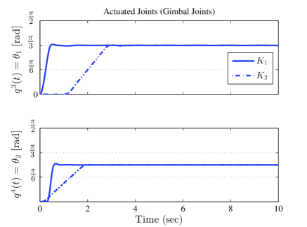
Figure 2: Time trajectories of the actuated variables, $\theta_{1}(t)$ and $\theta_{2}(t)$.

To demonstrate the self-recovery phenomenon in this case, we apply the control law in Lemma 2.8 to control $\theta_{1}$ and $\theta_{2}$ such that they move from 0 [rad] to $\frac{\pi}{3}$ [rad] and $\frac{\pi}{4}$ [rad], respectively, within 3 seconds; see Fig. 2. For the unactuated cyclic joints, $x$ and $y$, we simulate two different cases of damping matrix $K=(k_{\alpha\beta})_{1\leq\alpha,\beta\leq 2}$:

$$K_{1}=\begin{pmatrix}3&0\\ 0&3\end{pmatrix},\quad K_{2}=\begin{pmatrix}5+2\cos{x}&4\\ 4&4+2\cos y\end{pmatrix}.$$

Notice that $K_{1}$ and $K_{2}$ are the second-order derivative matrices of $U_{1}(x,y)=\frac{3}{2}\left(x^{2}+y^{2}\right)$ and $U_{2}(x,y)=\frac{1}{2}x^{2}+2(x+y)^{2}-2\cos x-2\cos y$, respectively. One can easily verify that both $U_{1}$ and $U_{2}$ satisfy assumptions A5) – A7) and equations (22) and (23).

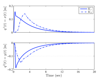
(a) Time trajectories.

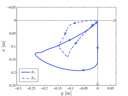
(b) $x-y$ plot.

Figure 3: Trajectories of unactuated cycle variables, $x(t)$ and $y(t)$.

The self-recovery phenomenon for both cases is verified in Fig. 3. From Fig. 3(a) and Fig. 2, one can see that $x(t)$ and $y(t)$ converge to the origin, which is the initial condition, after $\theta_{1}(t)$ and $\theta_{2}(t)$ settle down. The planar motion is described in Fig. 3(b), where we can clearly see the pendulum base automatically returns to its initial position for both cases.

3.2 Three-Link Manipulator on a Horizontal Plane

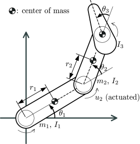
Figure 4: A three-link manipulator on a horizontal plane with $\theta_{1}$ and $\theta_{3}$ unactuated.

Consider the three-link open chain manipulator moving on a horizontal plane (i.e. no gravity effect) in Fig. 4. One can easily see that the first joint angle $\theta_{1}$ is a cyclic variable, which is always the case for planar kinematic chains whose motion is constrained to a horizontal plane. For this particular system in Fig. 4, the third joint angle $\theta_{3}$ is also cyclic since the center of mass of the third link is located on its axis of rotation. Thus, we anticipate the self-recovery effect will occur in these two joint variables. To be compatible with the notation introduced in Section 2, we choose the configuration variables as $q^{1}=\theta_{1}$, $q^{2}=\theta_{3}$ and $q^{3}=\theta_{2}$. Then, the mass matrix is written as

$${M}=\begin{pmatrix}\alpha+2\beta c_{2}&I_{3}&\delta+\beta c_{2}\\ I_{3}&I_{3}&I_{3}\\ \delta+\beta c_{2}&I_{3}&\delta\end{pmatrix},$$

where $c_{2}$ denotes $\cos{\theta_{2}}$, and parameters $\alpha$, $\beta$ and $\delta$ are given by

$$\begin{split}\alpha&=I_{1}+I_{2}+I_{3}+m_{1}r_{1}^{2}+m_{2}(\ell_{1}^{2}+r_{2}^{2})+m_{3}(\ell_{1}^{2}+\ell_{2}^{2}),\\ \beta&=\ell_{1}(m_{2}r_{2}+m_{3}\ell_{2}),\\ \delta&=I_{2}+I_{3}+m_{2}r_{2}^{2}+m_{3}\ell_{2}^{2},\end{split}$$

where individual parameter values are listed in Table 2. We use the following damping coefficient matrix:

$$K=\begin{pmatrix}6&0\\ 0&3\end{pmatrix}$$

which is the second-order derivative matrix of the function $U(\theta_{1},\theta_{3})=\frac{3}{2}\left(2\theta_{1}^{2}+\theta_{3}^{2}\right)$.

Table 2: Parameters for the three-link manipulator

	Parameter	Value	Unit
$\ell_{1}$	Link 1 length	0.5	[m]
$\ell_{2}$	Link 2 length	0.5	[m]
$r_{1}$	Location of link 1 center of mass	0.1	[m]
$r_{2}$	Location of link 2 center of mass	0.1	[m]
$I_{1}$	Link 1 moment of inertia	2	[$\textrm{kg}\cdot\textrm{m}^{2}$]
$I_{2}$	Link 2 moment of inertia	2	[$\textrm{kg}\cdot\textrm{m}^{2}$]
$I_{3}$	Link 3 moment of inertia	2	[$\textrm{kg}\cdot\textrm{m}^{2}$]
$m_{1}$	Link 1 mass	10	[kg]
$m_{2}$	Link 2 mass	10	[kg]
$m_{3}$	Link 3 mass	10	[kg]

Figure 5 plots the time trajectories of the joint angles. The top plot shows the controlled motion of the second joint $\theta_{2}$ while the second and the third present the time trajectories of the two unactuated joints $\theta_{1}$ and $\theta_{3}$, respectively. A tracking controller is designed according to (30) such that the actuated second joint $\theta_{2}$ makes sixteen full revolutions (i.e. $32\pi$ [rad]) during the first 8 seconds of time. The initial values for the joint angles are set to $\theta_{2}(0)=\frac{\pi}{3}$, and $\theta_{1}(0)=\theta_{3}(0)=0$. Figure 5 clearly shows that both of the unactuated cyclic variables $\theta_{1}$ and $\theta_{3}$ converge back to their initial positions right after $\theta_{2}$ is regulated at $32\pi$ [rad]. Note that $\theta_{1}$ returns back to its original position after having made two full turns, demonstrating that the self-recovery effect is global. Besides the self-recovery phenomenon, the trajectories of $\theta_{1}$ and $\theta_{3}$ in Fig. 5 also demonstrate the damping-induced boundedness derived in Theorem 2.5. More specifically, we can observe that $\theta_{1}$ and $\theta_{2}$ oscillate around $-4\pi$ and $-3\pi$, respectively while $\theta_{2}$ is still increasing.

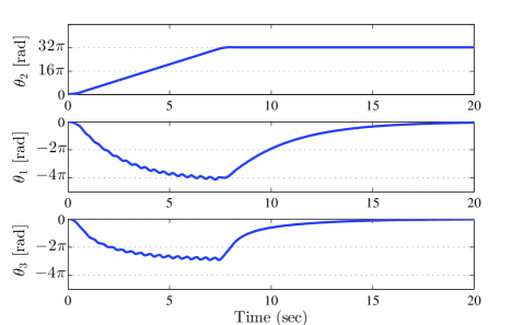
Figure 5: Time trajectories of joint angles, $\theta_{2}(t)$ (actuated), $\theta_{1}(t)$ (unactuated), and $\theta_{3}(t)$ (unactuated).

4 Conclusion and Future Work

The phenomena of damping-induced self-recovery and damping-induced boundedness have been generalized to mechanical systems with several unactuated cyclic variables. The major contribution of this paper comes from characterizing the damping coefficient matrix as the second-order derivative matrix of a function and identifying a class of such functions that guarantee the self-recovery and boundedness of all unactuated cyclic variables. Regular momentum conservation is the limit of the damping-induced self-recovery as the damping disappears, in the sense that the recovery phenomenon vanishes in the limit. Non-trivial examples of mechanical systems with multiple cyclic variables are provided to demonstrate the theoretical discoveries.

It will be interesting to study the possibility of occurrence of damping-induced self-recovery and boundedness for the case of non-Abelian symmetry in the unactuated variables. We are currently examining the system of a spacecraft with internal rotors, where the spacecraft experiences viscous damping friction as it rotates.

References

• [1] Chang, D. E., Jeon, S.: Damping-induced self recovery phenomenon in mechanical systems with an unactuated cyclic variable. ASME J. Dynamic Systems, Measurement,and Control 135(2), (2013). http://dx.doi.org/10.1115/1.4007556
• [2] Frohlich, C.: Do springboard divers violate angular momentum conservation? American Journal of Physics 47 (7), 583–592 (1979)
• [3] Gregg, R. D.: Geometric Control and Motion Planning for Three-Dimensional Bipedal Locomotion. Ph.D. dissertation. University of Illinois at Urbana-Champaign (2010)
• [4] Kane, T. R., Scher, M. P.: A dynamical explanation of the falling cat phenomenon. International Journal of Solids and Structures 55, 663–670 (1969)
• [5] Krishnaprasad, P. S.: Eulerian many-body problems. Contemporary Mathematics 97, 187–208 (1989)
• [6] Marsden, J.E., Montgomery, R., Ratiu, T.S.: Reduction, Symmetry, and Phases in Mechanics. Memoirs AMS 436 (1990)
• [7] Marsden, J.E., Ratiu, T.: Introduction to Mechanics and Symmetry: A Basic Exposition of Classical Mechanical Systems. Springer (1995)
• [8] Montgomery, R.: Gauge theory of the falling cat. Fields Institute Communications 1, 193–218 (1993)
• [9] Montgomery, R.: A Tour of Subriemannian Geometries, Their Geodesics and Applications. American Mathematical Society (2006)
• [10] Ruina, A.: Cats, astronauts, trucks, bikes, arrows, and muscle-smarts: Stability, translation, and rotation. Talk at Dynamic Walking 2010, http://video.mit.edu/watch/dynamic-walking-2010-andy-ruina-cats-astronauts-trucks-bikes-arrows-and-muscle-smarts-stabil-6010/
• [11] Spong, M. W.: Partial feedback linearization of underactuated mechanical systems. Proc. IEEE Conference on Intelligent Robots and Systems. Munich, Germany. 314–321 (1994)