Spinon and $\eta$-spinon correlation functions

Abstract

We calculate real-space static correlation functions related to basic entities of the one-dimensional Hubbard model, which emerge from the exact Bethe-ansatz solution. These entities involve complex rearrangements of the original electrons. Basic ingredients are operators related to unoccupied, singly occupied with spin up or spin down and doubly occupied sites. The spatial decay of their correlation functions is determined using an approximate mean-field-like approach based on the Zou-Anderson transformation and DMRG results for the half-filled case. The nature and spatial extent of the correlations between two sites on the Hubbard chain is studied using the eigenstates and eigenvalues of the two-site reduced density matrix.

1 Introduction

It was recently shown in [1] that a consistent description of the Bethe-ansatz exact eigenstates of the Hubbard chain can be achieved in terms of some basic entities called $c$ fermions, spinons and $\eta$-spinons. (In the related preliminary studies of [2] such objects were named $c$ pseudoparticles, spinons and holons, respectively.) These objects are related to the rotated-electron occupancy configurations. The rotated-electron creation and annihilation operators are related to those of the original electrons by a unitary transformation, $V(U)$. This transformation is defined such that double occupancy of these rotated electrons is a good quantum number for all values of $U$. There are infinite choices for such transformations. Examples are those reported in [3, 4]. However, the BA solution performs a specific electron - rotated-electron unitary transformation [1].

The operator formulation introduced in [1] accounts for all representations of the model global $[SO(4)\otimes U(1)]/Z_{2}$ symmetry algebra. Here $SO(4)=[SU(2)\otimes SU(2)]/Z_{2}$ refers to the spin $SU(2)$ and $\eta$-spin $SU(2)$ symmetries and $U(1)$ to the $c$ hidden $U(1)$ symmetry found in [5]. We denote the spin and the $\eta$-spin of an energy eigenstate by $S_{s}$ and $S_{\eta}$, respectively. We call $2S_{c}$ the number of rotated-electron singly occupied sites, which is the eigenvalue of the generator of the $c$ hidden $U(1)$ symmetry.

At very large $U$ double occupancy is a good quantum number, since there is a very large energy separation between states differing by the number of doubly occupied sites (in this limit the unitary transformation is the identity). As the Coulomb repulsion becomes finite, the unitary transformation is not known explicitly but it can be expressed in a perturbative expansion in powers of $t/U$, as shown for instance in [6]. To leading order in $t/U$ the unitary operators associated with such transformations have a universal form. Such operators differ in their higher-order terms. Recently, the matrix elements of the unitary operator associated with the specific transformation performed by the Bethe-ansatz solution has been obtained for the whole $U/t>0$ range in the basis of the energy eigenstates [1].

The various entities referred to above are introduced so that the number of $c$ fermions $N_{c}=2S_{c}$ and that of $c$ fermion holes $N_{c}^{h}=[N_{a}-2S_{c}]$ are equal to the number of singly occupied sites of rotated electrons (with spin up or spin down) and the number of rotated-electron doubly and unnocupied sites, respectively. They store information on the charge part of these rotated electrons. The number of spinons $M_{s}=2S_{c}$ also equals that of singly occupied sites of rotated electrons. The spin-$1/2$ spinons of component $+1/2$ have information on the spin of these rotated electrons of spin up, the spin-$1/2$ spinons of component $-1/2$ is related to the spin part of such rotated electrons with spin down. The number of $\eta$-spinons $M_{\eta}=[N_{a}-2S_{c}]$ equals that of rotated-electron doubly and unnocupied sites. While the $N_{c}^{h}=[N_{a}-2S_{c}]$ $c$ fermion holes describe the $c$ hidden $U(1)$ symmetry degrees of freedom of such sites occupancies, the $M_{\eta}=[N_{a}-2S_{c}]$ $\eta$-spinons refer to the $\eta$-spin $SU(2)$ symmetry degrees of freedom of the same site occupancies. Specifically, the $\eta$-spin-$1/2$ $\eta$-spinons of component $+1/2$ are related to the unoccupied occupied sites and the $\eta$-spin-$1/2$ $\eta$-spinons of component $-1/2$ are related to the doubly sites of the rotated electrons.

Furthermore in [1, 2] it was proposed that both the energy eigenstates inside and outside the Bethe-ansatz solution subspace can be generated by occupancy configurations of the $c$ fermions (associated with the usual real charge rapidities of the Bethe ansatz solution) and suitable spinon and $\eta$-spinon occupancy configurations.

Out of the $M_{s}=2S_{c}$ spinons, a number $M_{s}^{un}=2S_{s}$ of spinons are unbound and determine the energy eigenstate spin value $S_{s}$. For the energy eigenstates inside the Bethe-ansatz subspace, all unbound spinons have spin projection $+1/2$. Flipping such unbound spinons generates the spin towers of spin projection $S_{s}^{z}=-S_{s},-S_{s}+1,...,S_{s}-1,S_{s}$. The corresponding energy eigenstates are outside the Bethe-ansatz subspace. The remaining $M_{s}^{bo}=[2S_{c}-2S_{s}]$ spinons are bound within composite entities with total spin zero (bound-state between a spin-$1/2$ spinon with component $1/2$ and another spin-$1/2$ spinon with component $-1/2$). There are also Bethe-anstaz excited states containing $\nu=1,2,3,...$ spin-neutral pairs of such bound spinons. Note that zero-magnetization ground states have no unbound spinons, so that all their spinons are bound within spin-neutral pairs. In this case one has that $M_{s}=2N_{s1}$, where $N_{s1}$ is the number of spin-singlet two-spinon composite objects called in [1] $s1$ fermions.

Similarly, out of the $M_{\eta}=[N_{a}-2S_{c}]$ $\eta$-spinons, a number $M_{\eta}^{un}=2S_{\eta}$ of $\eta$-spinons are unbound and determine the energy eigenstate $\eta$-spin value $S_{\eta}$. For the energy eigenstates inside the Bethe-ansatz subspace, all unbound $\eta$-spinons have $\eta$-spin projection $+1/2$. Those correspond to rotated-electron unoccupied sites. Flipping such unbound $\eta$-spinons generates the $\eta$-spin towers of $\eta$-spin projection $S_{\eta}^{z}=-S_{\eta},-S_{\eta}+1,...,S_{\eta}-1,S_{\eta}$. Such $\eta$-spin flipping processes involve creation of on-site spin-neutral electron pairs of momentum $\pi$. The corresponding energy eigenstates are outside the Bethe-ansatz subspace. The remaining $M_{\eta}^{bo}=[N_{a}-2S_{c}-2S_{\eta}]$ $\eta$-spinons are anti-bound within composite entities with total $\eta$-spin zero (anti-bound state between a $\eta$-spin-$1/2$ $\eta$-spinon with component $1/2$ and another one with component $-1/2$). Again, there are as well Bethe-anstaz excited states containing $\nu=1,2,3,...$ $\eta$-spin-neutral pairs of such anti-bound $\eta$-spinons. Each pair involves two sites, doubly occupied and unoccupied by rotated electrons, respectively.

The eigenvalue $2S_{c}$ of the operator that counts the number of rotated-electron singly occupied sites obeys the inequality $2S_{c}\leq N$. As a simple example let us consider ground states with electronic density $n=N/N_{a}$ and spin density $m=[N_{\uparrow}-N_{\downarrow}]/N_{a}$ in the ranges $n\in(0,1)$ and $m\in(0,n)$, respectively. For such ground states one has that $2S_{c}=N$. Within the operator formulation of [1], those have $M_{s}=[M_{\eta}^{un}+M_{\eta}^{bo}]=N$ spinons of which $M_{s}^{un}=2S_{s}$ are unbound spinons and $M_{s}^{bo}=2N_{s1}$ are bound spinons inside $N_{s1}=[N/2-S_{s}]$ spin-neutral two-spinon composite $s1$ fermions. Furthermore, such ground states have $M_{\eta}=2S_{\eta}=[N_{a}-N]$ $\eta$-spinons, $N_{c}=N$ $c$ fermions, and $N_{c}^{h}=[N_{a}-N]$ $c$ fermion holes. For them the number of electrons $N$ equals that of rotated electrons that singly occupy sites and the number of rotated-electron doubly occupied sites vanishes. The ground-state $M_{s}=N$ spinons refer to the $N$ spin-$1/2$ spins of the rotated electrons that singly occupy sites. The ground-state $N_{c}=N$ $c$ fermions describe the charge degrees of freedom of such rotated electrons. The ground-state $M_{\eta}=[N_{a}-N]$ $\eta$-spinons describe the $\eta$-spin degrees of freedom of the $[N_{a}-N]$ sites unoccupied by rotated electrons. The ground-state $N_{c}^{h}=[N_{a}-N]$ $c$ fermion holes describe the $c$ hidden $U(1)$ symmetry degrees of freedom of the latter $[N_{a}-N]$ sites ground-state occupancies.

Consistent with the results briefly reported above, within the formulation of [1] the $\eta$-spin degrees of freedom of the rotated-electron unoccupied sites with component $1/2$ and the rotated-electron doubly occupied sites with component $-1/2$ tend to be anti-bound, whereas the singly occupied sites by electrons of opposite spin projection tend to be bound. One expects therefore correlations that should decrease somewhat fast with distance between the members of each pair of $\eta$-spinons or of spinons.

The relevance of the correlations between doubly occupied sites and unoccupied sites has been suggested before by several authors. This can involve the introduction of an effective low-energy theory that contains a charge 2e bosonic mode [7, 8, 9], which may be bound to a hole. The significance of short-range correlations between unoccupied and doubly occupied sites was, for instance, found in [10]. The proposal of (anti-)bound states of doubly occupied sites and unoccupied sites in the repulsive Hubbard model at half-filling (Mott insulating phase) and of spins of opposite projections in the negative case (Luther-Emery phase), were recently justified by the existence of long range-order in a non-local order parameter [11].

The unitary transformation, $V(U)$, is such that $[\tilde{D},H]=0$, where $\tilde{D}=VDV^{-1}=VDV^{\dagger}$, with $D$ the operator that counts the number of doubly occupied sites of the original electrons. At very large $U$, the eigenstates of the Hamiltonian may be labelled by the eigenvalue of $D$ and at finite $U$ they may be labbelled by that of $\tilde{D}$. The rotated electrons (and in general any operator written in terms of the rotated electrons) can be obtained in the form $\tilde{c}=VcV^{-1}$, $\tilde{c}^{\dagger}=Vc^{\dagger}V^{-1}$. The eigenstates of the Hamiltonian at any value of $U$ may be generated as,

$$|\psi_{U}\rangle=V|\psi_{U=\infty}\rangle$$ (1)

which uniquely defines the unitary transformation [1]. Therefore any correlation function of two operators $A$ and $B$ satisfies,

$$\langle\psi_{U=\infty}|AB|\psi_{U=\infty}\rangle = \langle\psi_{U}|VABV^{-1}|\psi_{U}\rangle$$ (2)

$$= \langle\psi_{U}|\tilde{A}\tilde{B}|\psi_{U}\rangle$$

As a consequence any correlation function of operators involving rotated electrons at finite $U$ may be obtained from the correlation function of the original electrons calculated at very large $U$. The form of the unitary transformation, $V$, is rather involved and contains infinite terms if expressed in terms of the original electron operators. However, to calculate their correlation functions it is enough to calculate the correlation function of the original electrons at large $U$, which greatly simplifies the problem. (As a consequence, the correlation function of $\tilde{A}\tilde{B}$ is independent of $U$.) It is the purpose of this work to calculate the real-space correlation functions of these objects.

In this paper we use several methods to determine these correlation functions such as a mean-field theory based on the Zou-Anderson transformation [12], a possible description in terms of an exact spin-charge-like separation of the original degrees of freedom introduced by Östlund-Granath [13] and the density matrix renormalization group (DMRG) technique.

The first issue considered in the following has to do with the definition of which correlations functions one wants to calculate. Those typically involve products of several electronic operators. Considering low energies, where a bosonization approach should apply, we expect that as the number of fields increases the absolute value of the correlation functions exponents should increase (considerably). In the metallic phase bosonization predicts a power-law decay with distance. (If the exponent is high then the extent of the correlation function should be very small). In the case of half-filling Umklapp scattering may change the behavior to an exponential decay. (However, if the exponent of the power-law decay is high the two behaviors will be to some extent similar). One of the aims of this work is to determine the exponents of these decays or their correlation lengths.

2 Correlation functions

The correlation function,

$$C_{1}(r)=\langle\left(1-n_{\uparrow}(r)\right)\left(1-n_{\downarrow}(r)\right)n_{\uparrow}(r=0)n_{\downarrow}(r=0)$$ (3)

and its connected function,

$$C_{1}^{c}(r)=C_{1}(r)-\langle\left(1-n_{\uparrow}(r)\right)\left(1-n_{\downarrow}(r)\right)\rangle\langle n_{\uparrow}(r=0)n_{\downarrow}(r=0)\rangle$$ (4)

contain information about the correlations between a unoccupied site (of the original electrons) at point $r$ and a doubly occupied site at the origin. This is a charge correlation function. It is related (at large $U$) with the proposed (anti-)bound states of $\eta$-spinons with opposite $\eta$-spin projections. Those refer to the $\eta$-spin degrees of freedom of pairs of rotated-electron doubly occupied and unoccupied sites.

The correlation function,

$$C_{2}(r)=\langle\left(1-n_{\uparrow}(r)\right)n_{\downarrow}(r)n_{\uparrow}(r=0)\left(1-n_{\downarrow}(r=0)\right)\rangle$$ (5)

and its connected function,

$$C_{2}^{c}(r)=C_{2}(r)-\langle\left(1-n_{\uparrow}(r)\right)n_{\downarrow}(r)\rangle\langle n_{\uparrow}(r=0)\left(1-n_{\downarrow}(r=0)\right)\rangle$$ (6)

are related (at large $U$) with the proposed bound states of spinons with opposite spin projections. This is a spin-like correlation function. Even though the connection to the Bethe-ansatz states is through the rotated electrons, and only in the large $U$ limit they are close to the original electrons, we will consider in this work the correlation functions at different values of $U$.

We also calculate some mixed correlations where at point $r$ we have for instance a doubly occupied site and at site $r=0$ a singly occupied site, or at site $r$ a unoccupied site and at site $r=0$ a singly occupied site. That is we also calculate, for instance,

$$C_{3}(r)=\langle\left(1-n_{\uparrow}(r)\right)\left(1-n_{\downarrow}(r)\right)n_{\uparrow}(r=0)\left(1-n_{\downarrow}(r=0)\right)\rangle$$ (7)

or

$$C_{4}(r)=\langle n_{\uparrow}(r)n_{\downarrow}(r)n_{\uparrow}(r=0)\left(1-n_{\downarrow}(r=0)\right)\rangle$$ (8)

and the corresponding connected correlation functions.

The operator that counts the number of doubly occupied sites may be written as $\sum_{r}c_{r,\uparrow}^{\dagger}c_{r,\uparrow}c_{r,\downarrow}^{\dagger}c_{r,\downarrow}$, and similarly for the unoccupied sites $\sum_{r}c_{r,\uparrow}c_{r,\uparrow}^{\dagger}c_{r,\downarrow}c_{r,\downarrow}^{\dagger}$, singly occupied sites with spin up $\sum_{r}c_{r,\uparrow}^{\dagger}c_{r,\downarrow}c_{r,\downarrow}^{\dagger}c_{r,\uparrow}$ and singly occupied sites with spin down $\sum_{r}c_{r,\downarrow}^{\dagger}c_{r,\uparrow}c_{r,\uparrow}^{\dagger}c_{r,\downarrow}$. The evaluation of the correlation functions depends on the band-filling. Away from half-filling (metallic phase) we expect from the bosonisation that both the charge and the spin correlation functions will decay with distance, as power laws. At half filling it is expected that the charge correlation functions become exponential-like, due to the presence of a charge gap. In finite magnetic field the spin degrees of freedom will also develop a gap.

The corresponding correlation functions are then expected to be of the form,

$$C(r)\sim\frac{1}{r^{\sigma}}e^{-\frac{r}{\xi}}$$ (9)

for the charge correlation functions, if there is a charge gap such as at half-filling, where $\xi$ is the correlation length, and with a possible extra oscillating factor of the type $(-1)^{r}$. On the other hand, the spin correlation functions and the charge correlation functions in the metallic phase are expected to be of the form,

$$C(r)\sim\frac{1}{r^{\alpha}}[\ln r]^{\beta}$$ (10)

also with a possible extra oscillating factor of the type $(-1)^{r}$.

In the half-filling case and in the limit of large $U$ the spin part of the Hubbard model reduces to the spin-$1/2$ isotropic Heisenberg chain. Also the charge part is gapped. Previous studies for the charge correlations suggest that $\sigma\sim 1/2$. The study of the spin-spin correlation functions at half-filling lead to some controversy about the presence of logarithmic corrections, but the presence of a logarithmic factor with exponent $\beta=0.5$ was confirmed and the above $\alpha$ exponent reading $\alpha\sim 1$ [14, 15, 16, 17, 18].

There are transformations proposed in the literature that lead to a similar decoupling of the electronic degrees of freedom. Examples are for instance given in [12] or in [19]. The main motivation was the study of either the large-$U$ limit in the Hubbard or Anderson models [20], with the intent of controlling in a efficient way the projection to states where double occupancy is restricted (as in the $t-J$ model), but considering a finite value of $U$ instead of the extreme case of infinite $U$, usually taken care of by a single slave boson [21]. Both representations introduce explicitly operators related to the four possible states associated with each site. Namely that a site may be unoccupied, singly ocuppied with a given spin projection or douby occupied. In the Kotliar and Ruckenstein procedure four bosonic operators are added, enlarging the operator space, that act as projectors on the original fermionic operators. In the Zou-Anderson transformation the original electron operators are replaced by two sets of two bosonic and fermionic operators that fulfill the projection. However, both representations lead to an enlargement of the physical Hilbert space and the extra unphysical states have to be projected out. We note, however, that the representation introduced by Zou and Anderson (ZA) has been used to explicitly obtain an exact solution of the Hubbard model in the large $U$ limit in a much simpler way as compared to the Bethe ansatz [22]. Also, it has been used to study the stiffness of the one-dimensional Hubbard model in a way equivalent and alternative to the Bethe-ansatz solution [23].

2.1 Zou-Anderson transformation

The electron operators may be written as,

$$c_{i,\sigma} = e_{i}^{\dagger}S_{i,\sigma}+\sigma S_{i,-\sigma}^{\dagger}d_{i}$$

$$c_{i,\sigma}^{\dagger} = S_{i,\sigma}^{\dagger}e_{i}+\sigma d_{i}^{\dagger}S_{i,-\sigma}$$ (11)

where the operators $e_{i},d_{i},S_{i,\sigma}$ annihilate sites that are unoccupied, doubly-occupied and singly-occupied with an electron with spin $\sigma$, respectively. Since the electron operators are fermionic we can either choose the operators $e,d$ as bosonic and the operators $S_{i,\sigma}$ as fermionic, or vice-versa. In the original paper [12] the first choice was made (called slave-boson approach) and in [22] the second choice was taken (called slave-fermion approach). Most expressions are the same, formally, in either case. The difference arises when one integrates over degrees of freedom or in the mean-field approach when the Bose-Einstein or the Fermi-Dirac distributions appear.

The enlargement of the degrees of freedom imposes the constraint,

$$e_{i}^{\dagger}e_{i}+d_{i}^{\dagger}d_{i}+\sum_{\sigma}S_{i,\sigma}^{\dagger}S_{i,\sigma}=1$$ (12)

at each site. (This is the completeness relation of the four possibilities: one site is either unoccupied, doubly-occupied, or is singly occupied by an electron with spin-up or down). The constraint is simply obtained imposing the anticommutation relation $\{c_{i,\sigma},c_{i,\sigma}\}=1$ and considering either the slave-bosons or slave-fermions commutation or anticommutation relations.

Let us consider the Hubbard model written as,

$$H=-t\sum_{i,\delta;\sigma}c_{i,\sigma}^{\dagger}c_{i+\delta,\sigma}+U\sum_{i}n_{i,\uparrow}n_{i,\downarrow}-\mu\sum_{i,\sigma}c_{i,\sigma}^{\dagger}c_{i,\sigma}$$ (13)

The first is the hopping term between a site $i$ and its neighbors distant by $\delta$ (in general vectors in a $d$-dimensional space), $U$ is the on-site repulsion and $\mu$ the chemical potential enforcing the band filling.

In terms of the slave-bosons or slave-fermions the Hubbard Hamiltonian may be rewritten as,

$$H = -t\sum_{i,\delta;\sigma}\left(e_{i}e_{i+\delta}^{\dagger}-d_{i}d_{i+\delta}^{\dagger}\right)S_{i,\sigma}^{\dagger}S_{i+\delta,\sigma}$$ (14)

$$- t\sum_{i,\delta}\left(e_{i}d_{i+\delta}(S_{i\uparrow}^{\dagger}S_{i+\delta,\downarrow}^{\dagger}-S_{i\downarrow}^{\dagger}S_{i+\delta,\uparrow}^{\dagger})+d_{i}^{\dagger}e_{i+\delta}^{\dagger}(S_{i\downarrow}S_{i+\delta,\uparrow}-S_{i\uparrow}S_{i+\delta,\downarrow})\right)$$

$$+ U\sum_{i}d_{i}^{\dagger}d_{i}+\mu\sum_{i}\left(e_{i}^{\dagger}e_{i}-d_{i}^{\dagger}d_{i}\right)-\mu N_{a}$$

The ZA mapping reverses the role of the interacting and kinetic terms in the Hamiltonian. The interacting Hubbard term becomes quadratic in the ZA particles and the kinetic one is transformed into an interacting quartic term that couples particles along the lattice links. This is particularly useful to study the strongly interacting (large $U$) regime where the kinetic term is treated as a perturbation. The price of this transformation is the appearance of an on-site constraint, which assures exactly one particle per lattice site. In the mean field (MF) approach this translates to an on-site Lagrange multiplier.

The problem to be solved involves the effective Hamiltonian,

$$H = -t\sum_{i,\delta;\sigma}\left(e_{i}e_{i+\delta}^{\dagger}-d_{i}d_{i+\delta}^{\dagger}\right)S_{i,\sigma}^{\dagger}S_{i+\delta,\sigma}$$ (15)

$$- t\sum_{i,\delta}\left(e_{i}d_{i+\delta}(S_{i\uparrow}^{\dagger}S_{i+\delta,\downarrow}^{\dagger}-S_{i\downarrow}^{\dagger}S_{i+\delta,\uparrow}^{\dagger})+d_{i}^{\dagger}e_{i+\delta}^{\dagger}(S_{i\downarrow}S_{i+\delta,\uparrow}-S_{i\uparrow}S_{i+\delta,\downarrow})\right)$$

$$+ U\sum_{i}d_{i}^{\dagger}d_{i}+\mu\sum_{i}\left(e_{i}^{\dagger}e_{i}-d_{i}^{\dagger}d_{i}\right)-\mu N$$

$$+ \sum_{i}\lambda_{i}\left(e_{i}^{\dagger}e_{i}+d_{i}^{\dagger}d_{i}+\sum_{\sigma}S_{i,\sigma}^{\dagger}S_{i,\sigma}-1\right)$$

where we have introduced at each site a Lagrange multiplier, $\lambda_{i}$, to inforce the constraint. The transformation of the electron operators to the auxiliary operators already embodies part of the classification of the Bethe-ansatz states (actually for the rotated electrons). It seems therefore natural to decouple the quartic terms in the Hamiltonian in such a way that the unoccupied and doubly-occupied sites are separated, on a first stage, from the singly-occupied sites. Also, we consider that the unoccupied sites and the doubly-occupied sites are paired on nearest-neighbor links. On the other hand, the spin states of the singly-occupied sites are paired into spin singlets.

We then consider the mean-field Hamiltonian in the following form [24],

$$H_{MF}=-t\sum_{i,\delta;\sigma}\left\{\left(\chi_{\delta}^{e}-\chi_{\delta}^{d}\right)S_{i,\sigma}^{\dagger}S_{i+\delta,\sigma}\right.$$

$$+\left.\left(e_{i+\delta}^{\dagger}e_{i}-d_{i+\delta}^{\dagger}d_{i}\right)\chi_{\delta,\sigma}^{S}-\left(\chi_{\delta}^{e}-\chi_{\delta}^{d}\right)\chi_{\delta,\sigma}^{S}\right\}$$

$$-t\sum_{i,\delta}\left\{\Phi_{\delta}\left(S_{i\uparrow}^{\dagger}S_{i+\delta,\downarrow}^{\dagger}-S_{i\downarrow}^{\dagger}S_{i+\delta,\uparrow}^{\dagger}\right)+\Phi_{\delta}^{*}\left(S_{i\downarrow}S_{i+\delta,\uparrow}-S_{i\uparrow}S_{i+\delta,\downarrow}\right)\right.$$

$$\left.+e_{i}d_{i+\delta}\Delta_{\delta}^{*}+d_{i}^{\dagger}e_{i+\delta}^{\dagger}\Delta_{\delta}-\Phi_{\delta}\Delta_{\delta}^{*}-\Phi_{\delta}^{*}\Delta_{\delta}\right\}$$

$$+U\sum_{i}d_{i}^{\dagger}d_{i}+\mu\sum_{i}\left(e_{i}^{\dagger}e_{i}-d_{i}^{\dagger}d_{i}\right)-\mu N$$

$$+\sum_{i}\lambda_{i}\left(e_{i}^{\dagger}e_{i}+d_{i}^{\dagger}d_{i}+\sum_{\sigma}S_{i,\sigma}^{\dagger}S_{i,\sigma}-1\right)$$ (16)

The quantities appearing in this Hamiltonian expression are defined as follows,

$$\chi_{\delta}^{e} = \langle e_{i+\delta}^{\dagger}e_{i}\rangle$$

$$\chi_{\delta}^{d} = \langle d_{i+\delta}^{\dagger}d_{i}\rangle$$

$$\chi_{\delta,\sigma}^{S} = \langle S_{i,\sigma}^{\dagger}S_{i+\delta,\sigma}\rangle$$

$$\Phi_{\delta} = \langle e_{i}d_{i+\delta}\rangle$$

$$\Delta_{\delta} = \langle\left(S_{i,\downarrow}S_{i+\delta,\uparrow}-S_{i,\uparrow}S_{i+\delta,\downarrow}\right)\rangle$$ (17)

Besides considering hopping amplitudes we also introduce two pairing terms [24], one between the unoccupied and doubly-occupied sites and another one between singly occupied sites with opposite spins. Note that one refers to a boson pairing and the other to a fermionic pairing. The choice of the mean-field parameters has in mind the possible bound states between the $e$ and $d$ operators and the $S_{\uparrow}$ and $S_{\downarrow}$ operators. Indeed, we intend to investigate the tendency to form these bound-states. The problem is now quadratic and may be diagonalized. The solution is briefly reviewed in Appendix A.

Generically the phases found by solving the MF solutions for arbitrary band filling and energy are characterized as follows [24]: Phase (1) is conducting and characterized by $\chi\neq 0,\ \Delta=0$. In it the spinons are gapless and the charge degrees of freedom exibit a gap of the order of the temperature, which closes at $T=0$. This is the lowest free-energy phase. Within the mean-field approach it is that corresponding to the ground state. At finite energies other phases emerge [24], such as phase (2) $\chi=0,\ \Delta\neq 0$, which is gapped for both degrees of freedom. Since it appears near $x=0$ it is tempting to identify it with an insulating antiferromagnet. Phase (3) $\chi\neq 0,\ \Delta\neq 0$ is a precursor of the superconductor. In it there exists spin-singlet formation but the charge motion is incoherent since no condensation is allowed. If one imposes $e_{k=0}=Z$, this phase splits into two sub-phases, analog to the pseudogap and superconducting phases in [25]. Phase (4) is an incoherent high-temperature phase where all correlations are zero.

The hopping and pairing correlation functions between two sites at distance $r$ from each other are given by,

$$\chi_{F}(r) = \left\langle\mathit{s}_{r,1}^{\dagger}\mathit{s}_{0,1}+\mathit{s}_{r,-1}^{\dagger}s_{0,-1}\right\rangle_{0},$$

$$\Delta_{F}(r) = \left\langle\mathit{s}_{r,1}\mathit{s}_{0,-1}-\mathit{s}_{r,-1}\mathit{s}_{0,1}\right\rangle_{0},$$

$$\chi_{B}(r) = \left\langle\mathit{d}_{r}^{\dagger}\mathit{d}_{0}-\mathit{e}_{r}^{\dagger}\mathit{e}_{0}\right\rangle_{0},$$

$$\Delta_{B}(r) = \left\langle\mathit{d}_{r}\mathit{e}_{0}+\mathit{e}_{r}\mathit{d}_{0}\right\rangle_{0}.$$ (18)

They have been calculated before in Ref. [24] for the various phases. Although these correlation functions are not gauge invariant, they are useful to characterize the different phases. For phases (1) and (3) and both for the fermion and the boson hopping correlation functions, it was found close to half filling that the correlation length increases as the doping increases [24]. Particularly, the bosonic correlation function has a large correlation length. Analyzing the correlation length of $\Delta_{B}$, one clearly sees a long-range correlation in the high doping regime ($x=1-n$ large), possibly precursor of Bose-condensation and superconductivity. In the low-doping region, both the bosonic and the fermionic correlation functions have a smaller range consistent with a spin gapped state. In this regime the two correlation functions have similar range, while at higher doping the charge correlation function has a much larger range compared to the spin correlation function. These correlation functions will be relevant if the system is in a deconfined phase. In a confined phase these correlation functions loose their significance, as the various degrees of freedom are confined within the real electrons. However, use of the Bethe-ansatz solution reveals that some fractionalization and rearrangement of the degrees of freedom occurs.

We can now calculate the above mentioned correlation functions, $C_{1}(r),C_{2}(r)$, in the mean-field approach.

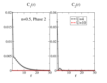
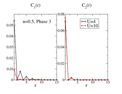
Figure 1: Correlation functions $C_{1}^{c}(r),C_{2}^{c}(r)$ for $n=0.5$, $U=4,10$ and $N=100$ in the phases 2 and 3.

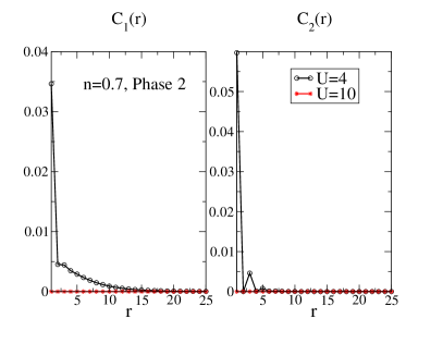
Figure 2: Correlation functions $C_{1}^{c}(r),C_{2}^{c}(r)$ for $n=0.7$, $U=4,10$ and $N=100$ in the phases 2 and 3.

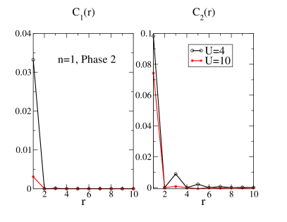
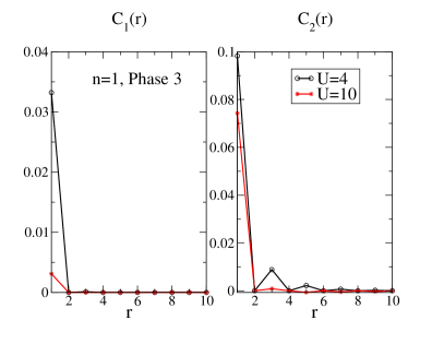
Figure 3: Correlation functions $C_{1}^{c}(r),C_{2}^{c}(r)$ for $n=1$, $U=4,10$ and $N=100$ in the phases 2 and 3.

Using the constraint we can write that,

$$C_{1}(r) = \langle\left(1-n_{\uparrow}(r)\right)\left(1-n_{\downarrow}(r)\right)n_{\uparrow}(r=0)n_{\downarrow}(r=0)\rangle=\langle n_{e}(r)n_{d}(0)\rangle$$

$$C_{2}(r) = \langle\left(1-n_{\uparrow}(r)\right)n_{\downarrow}(r)n_{\uparrow}(r=0)\left(1-n_{\downarrow}(r=0)\right)\rangle=\langle n_{s\downarrow}(r)n_{s\uparrow}(0)\rangle$$

and the corresponding connected functions read,

$$C_{1}^{c}(r) = \langle n_{e}(r)n_{d}(0)\rangle-\langle n_{e}(r)\rangle\langle n_{d}(0)\rangle$$

$$C_{2}^{c}(r) = \langle n_{s\downarrow}(r)n_{s\uparrow}(0)\rangle-\langle n_{s\downarrow}(r)\rangle\langle n_{s\uparrow}(0)\rangle$$ (20)

where $n_{e}=e^{\dagger}e$, $n_{d}=d^{\dagger}d$, $n_{s\uparrow}=s_{\uparrow}^{\dagger}s_{\uparrow}$ and $n_{s\downarrow}=s_{\downarrow}^{\dagger}s_{\downarrow}$. Using their representations in momentum space in terms of the diagonalized operators we obtain the results derived in Appendix A. Those are shown in Figs. 1 and 2.

At half filling we are in the insulating phase (2). We expect therefore a charge gap and an exponential decay of the correlation function $C_{1}(r)$. This is indeed seen for the values of $U=4,10$, and independentely of the system size, where the spatial extent refers basically to nearest-neighbors. The spin part is gapless, so that a larger range correlation function is expected, as shown in Fig. 3. As $U$ increases, the magnitude of $C_{2}(r)$ grows for $r=1$, but decreases faster with distance as compared to smaller values of $U$. Away from half filling we consider the densities $n=0.7,0.5$. In the metallic phase the charge correlation function has a much larger range, comparable to or larger than the spin counterpart. This qualitatively agrees with the results for the non-gauge invariant correlations. Far from half filling (quarter filling, $n=0.5$) the spin correlations decrease fast with distance since we move far from the half-filled antiferromagnet.

As stated above, there are two sorts of approximations within the present approach. The first is related to the enlargment of the physical Hilbert space and the necessity of introducing a constraint, to reduce the system to that space. The other sort of approximation has to do with the mean-field approach used. Moreover, the constraint is only implemented on average, as usual in slave-boson or slave-fermion approaches.

The first difficulty has been overcome recently [13], with the introduction of an exact transformation of the electron operators in terms of other operators that are related to the spin-charge separation of the model. The electron operators can be written as composites of charge-like and spin-like operators that do not give rise to any unphysical states, and thus avoids introducing any constraint.

2.2 Östlund-Granath transformation

This transformation [13] introduces new operators called quasicharge ${\hat{c}}^{\phantom{\dagger}}_{r}$ and quasispin operators $q^{i}_{r}$ that obey, respectively, Fermi and Bose statistics,

$${\hat{c}}^{\phantom{\dagger}}_{r} = c^{\dagger}_{\uparrow,\,r}(1-n_{\downarrow,\,r})+(-1)^{r}c^{\phantom{\dagger}}_{\uparrow,\,r}n_{\downarrow,\,r}$$ (21)

$$q^{+}_{r} = (c^{\dagger}_{\uparrow,\,r}-(-1)^{r}c^{\phantom{\dagger}}_{\uparrow,\,r}\;)\;c^{\phantom{\dagger}}_{\downarrow,\,r}$$ (22)

$$q^{-}_{r} = (q^{+}_{r})^{\dagger}$$

$$q^{z}_{r} = \textstyle{{\textstyle\frac{1}{2}}}-n_{\downarrow,\,r}$$

These operators satisfy the algebra $\{{\hat{c}}^{\phantom{\dagger}}_{r},{\hat{c}}^{\dagger}_{{r^{\prime}}}\}=\delta_{r,{r^{\prime}}}$ , $\{{\hat{c}}^{\dagger}_{r},{\hat{c}}^{\dagger}_{{r^{\prime}}}\}=0$ , $\left[\,{\hat{c}}^{\dagger}_{r},q^{i}_{{r^{\prime}}}\,\right]=0$ , $\left[\,q^{i}_{r},q^{j}_{{r^{\prime}}}\right]=i\delta_{r{r^{\prime}}}\sum_{k}\epsilon_{ijk}q^{k}_{r}$. The electron operators are expressed in terms of them as,

$$c^{\dagger}_{\uparrow,\,r} = {\hat{c}}^{\phantom{\dagger}}_{r}\;(\,{\textstyle\frac{1}{2}}+q^{z}_{r})\;+\;(-1)^{r}\;{\hat{c}}^{\dagger}_{r}({\textstyle\frac{1}{2}}-q^{z}_{r})$$ (23)

$$c^{\dagger}_{\downarrow,\,r} = q^{-}_{r}\,(\,{\hat{c}}^{\phantom{\dagger}}_{r}\;-\;(-1)^{r}\,{\hat{c}}^{\dagger}_{r}\,).$$

The Östlund-Granath representation involves other operators such as the quasicharge operator $n^{c}_{r}={\hat{c}}^{\dagger}_{r}{\hat{c}}^{\phantom{\dagger}}_{r}$ and the local pseudospin operators $p^{i}_{r}=n^{c}_{r}q^{i}_{r}$, which are the generators of the $SU(2)$ algebra that corresponds to ”rotations” between the unoccupied and doubly occupied states [26].

The following results hold $n_{r}=1-2n^{c}_{r}q^{z}_{r}$, $s^{i}_{r}=(1-n^{c}_{r}\,)\;q^{i}_{r}$ and $n^{c}_{r}=(n_{r}-1)^{2}$ where $s^{i}_{r}={\textstyle\frac{1}{2}}\sum_{\alpha,\beta}c^{\dagger}_{\alpha,\,r}\sigma^{i}_{\alpha\beta}c^{\phantom{\dagger}}_{\beta,\,r}$, with $\sigma^{i}$ the Pauli matrices. The total z-component of pseudospin can therefore be seen to be half the number of doubly occupied sites minus the number of unoccupied sites, which is precisely the charge relative to half filling. The action of these operators onto the four-state basis is shown in Fig. 4.

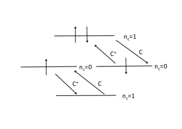
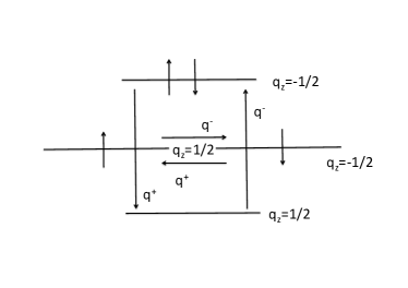
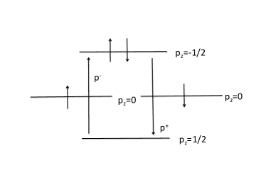
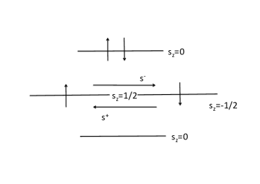
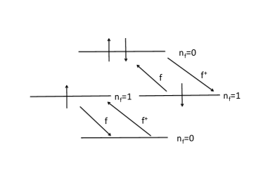
Figure 4: Eigenvalues of the quasicharge, quasispin, pseudospin and spin for each of the four basis states referring to a doubly occupied site, singly occupied site with spin up and spin down and unoccupied site. The transitions generated by the off-diagonal operators are also shown. In the last panel we consider the transitions generated by $n_{f}=1-n_{c}$ where $f=c^{\dagger},f^{\dagger}=c$, similarly to the operators introduced in [28] (for the rotated electrons).

The Hubbard model can be rewritten in terms of the quasiparticle operators as,

$$H=t\;({T_{0}}+{T_{1}}+{T_{-1}})+Uh_{U}$$ (24)

with $h_{U}={\textstyle\frac{1}{2}}\sum_{r}\,{\hat{c}}^{\dagger}_{r}{\hat{c}}^{\phantom{\dagger}}_{r}$,

$${T_{0}} = \frac{1}{2}\sum_{\rme{r,{r^{\prime}}}}\,(1+4{\bm{q}}_{\,r}\cdot{\bm{q}}_{\,{r^{\prime}}})({\hat{c}}^{\dagger}_{r}{\hat{c}}^{\phantom{\dagger}}_{{r^{\prime}}}+CC)$$ (25)

$${T_{1}} = \frac{1}{2}\sum_{\rme{r,{r^{\prime}}}}(-1)^{r}\,(1-4{\bm{q}}_{\,r}\cdot{\bm{q}}_{\,{r^{\prime}}})({\hat{c}}^{\dagger}_{r}{\hat{c}}^{\dagger}_{{r^{\prime}}})$$

and $T_{-1}=T_{1}^{\dagger}$.

Even though this transformation achieves some sort of exact spin-charge separation (actually quasispin and quasicharge), the Hamiltonian has a complicated structure. Although it has quartic interacting terms, since they involve the quasispin operators, these are typically represented in terms of bilinear representations of fermionic or bosonic operators. Usually these representations enlarge the physical Hilbert space and one has to introduce constraints. One can use a Majorana fermion representation [27] but this leads to an Hamiltonian where the leading interacting term involves six operators and, therefore, the analytical treatment is rather complicated. One can also represent the quasispin operators using the Jordan-Wigner transformation. The transverse terms are linear in terms of new fermionic operators (the strings cancel out since only nearest-neighbor hoppings are considered) but the longitudinal term is again a bilinear in fermionic operators (which leads again to terms with six operators). An analytical treatment would need some approximation scheme, which is known to not yield good results in one-dimensional systems.

It is interesting however to look at the behavior of the correlation functions of these operators. Moreover, it has been shown that the quasicharge operator is associated with a recently found hidden $U(1)$ symmetry of the Hubbard model [5] (on any bipartite lattice). Together with the exact Bethe-ansatz solution of the 1D problem, such a symmetry has lead to a deeper understanding of the physics of the model, including an understanding of the dressed scattering matrix structure [1]. Specifically, we are interested in the correlation functions for the quasicharge and the quasispin operators of Östlund and Granath written in terms of the original electron operators (and the corresponding connected correlation functions),

$$C_{5}(r)=\langle n_{c}(r)n_{c}(0)\rangle = \langle\left(n(r)-1\right)^{2}\left(n(0)-1\right)^{2}\rangle$$

$$C_{6}(r)=\langle\left(1-n_{c}(r)\right)\left(1-n_{c}(0)\right)\rangle = 1-\langle n_{c}(r)\rangle-\langle n_{c}(0)\rangle+\langle n_{c}(r)n_{c}(0)\rangle$$

$$C_{7}(r)=\langle q_{z}(r)q_{z}(0)\rangle = \langle\left(\frac{1}{2}-n_{\downarrow}(r)\right)\left(\frac{1}{2}-n_{\downarrow}(0)\right)\rangle$$

where $n(r)=n_{\uparrow}(r)+n_{\downarrow}(r)$ and $n_{\sigma}=c^{\dagger}_{\sigma}c_{\sigma}$.

We may also rewrite the pseudospin correlation functions in terms of the original electron operators (and the corresponding connected correlation functions),

$$C_{8}(r) = \langle p_{z}(r)p_{z}(0)\rangle=\langle\left(n(r)-1\right)^{2}\left(\frac{1}{2}-n_{\downarrow}(r)\right)\left(n(0)-1\right)^{2}\left(\frac{1}{2}-n_{\downarrow}(0)\right)\rangle$$

The spin correlation function can be evaluated in the usual way,

$$C_{9}(r)=\langle s_{z}(r)s_{z}(0)\rangle$$ (28)

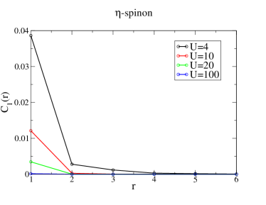
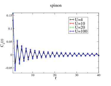
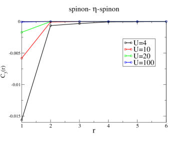
Figure 5: Connected correlation functions $C_{1}$ ($\eta$-spinon), $C_{2}$ (spinon), $C_{3}$ and $C_{4}$ (spinon-$\eta$-spinon).

A direct solution of these correlation functions in terms of the Östlund and Granath Hamiltonian is complicated, since even the mean-field approach is complex. Therefore, we have used a DMRG method to calculate these and other correlation functions.

2.3 DMRG calculations: Correlation functions

For simplicity, here we limit ourselves to the half-filling case. Using the DMRG method (briefly reviewed in Appendix B) we have calculated the correlation functions indicated above. We consider correlation functions for the original electron operators as a function of $U$. We emphasize that in the limit of very large $U$ these equal the correlation functions of the rotated electrons for $U>0$.

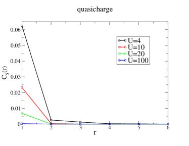
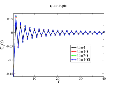
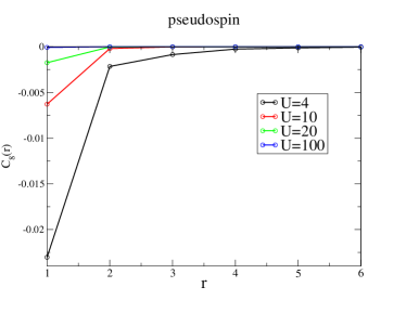
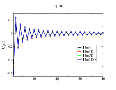
Figure 6: Connected correlation functions $C_{5}$ (quasicharge), $C_{7}$ (quasispin), $C_{8}$ (pseudospin) and $C_{9}$ (spin).

The charge correlation functions typically decay fast as the distance $r$ between the two operators grows. On the other hand, the spin related correlation functions oscillate by a factor of the type $(-1)^{r}$ and decay slowly with distance with a power law behavior, like in the spin-$1/2$ isotropic Heisenberg model.

In Fig. (5) we present results for the correlations functions $C_{1}$, $C_{2}$, $C_{3}$ and $C_{4}$. The correlation function $C_{1}(r)$ decays fast with distance, which shows that the doubly occupied sites and the unoccupied sites are tightly correlated in the half-filled phase. As $U$ grows the spatial extent is strongly reduced and in the large $U$ limit the correlation is basically extended to the nearest-neighbors. Since in the very large $U$ limit a doubly occupied site costs an infinite energy, the correlation function basically vanishes. The very large $U$ limit corresponds to the correlation function of the rotated electrons for the whole $U>0$ range. Hence this implies a very short range and a vanishing correlation function in the strictly infinite limit.

The correlation functions for the doubly occupied sites and a singly occupied site or a unoccupied site and a singly occupied site are negative. This is indicative of an anti-correlation, as expected. These correlations also decay very fast with distance.

On the other hand, the correlation function $C_{2}(r)$ for a singly-occupied site with spin up and a singly occupied site with opposite spin projection, is somewhat similar to the longitudinal spin correlation function. It oscillates with distance and decays slowly with $r$, which indicates a long-range correlation. The influence of the Hubbard interaction is smaller than for the charge correlation functions. For large $U$ the short range values of the correlation function increases, consistently with a more pronounced spin character of the excitations of the half-filled Hubbard model at large interactions. However, as $U$ becomes very large (for instance comparing $U=100$ with $U=20$) the decay with distance is faster.

In Fig. (6) we show results for the correlation functions for the quasicharge, quasispin and pseudospin operators introduced in Ref. [13]. The charge correlation functions decay fast in a way similar to $C_{1}(r)$, specifically the quasicharge and the pseudospin correlation functions. The quasicharge shows a correlation while the pseudospin shows an anti-correlation. The two spin correlation functions have a slowly decaying oscillating behavior. Analysis of both the quasispin and the spin correlation functions reveals that the nearest-neighbor is anti-correlated. On the other hand, the spinon correlation function $C_{2}(r)$ behavior shows that the nearest-neighbors are positively correlated, since it is an occupation number correlation function. The other correlation functions respect the opposite spin projections.

The charge correlation functions can be fitted with an expression of the form given in Eq. (9). Both the decay length $\xi$ and the exponent $\sigma$ are indicative of a stronger decay as the coupling grows. The results are shown in the Table.

$$\begin{array}[]{lllll}&U=4&U=10&U=20&U=100\\ \sigma&2.16&4.84&6.43&11.17\\ \xi&2.03&1.39&1.&1.\end{array}$$

The spin correlation functions can be fitted to an expression of the form provided in Eq. (10). The results for the various spin related correlation functions show that their decay is very similar to the decay of the spin correlation function $C_{9}(r)$. In the infinite $U$ limit these correlation functions tend to the corresponding correlation functions of the spin-$1/2$ isotropic Heisenberg model.

2.4 Eigenstates of the reduced density matrix

The correlation functions we have calculated give information on the correlations between the various entities discussed above. A more direct approach is obtained studying the eigenstates and eigenvalues of the reduced density matrix of two sites in the chain. Considering a chain of $N$ sites we may single out two sites distant by $r$ lattice units. The full density matrix of the chain can then be written as,

$$\rho_{N}=|\psi\rangle\langle\psi|$$ (29)

where $|\psi\rangle$ is the ground state of the system. The ground state may be written as the direct product of the states at each site. These can be written in terms of a basis with four states, namely $|\phi\rangle=|0\rangle,|\uparrow\rangle,|\downarrow\rangle,|\uparrow\downarrow\rangle$, referring to the four possibilities that each site is either unoccupied, occupied by a particle of spin up, a particle of spin down or doubly occupied, respectively. The full density matrix is a $4^{N}\times 4^{N}$ matrix. The ground state may be obtained for instance considering exact diagonalization of small systems. We have used Lanczos method to obtain the ground state expressed in this basis. We considered a system of size $N=14$.

Information about the correlation between two points on the lattice may be obtained considering a reduced density matrix by integrating $N-2$ sites. One of the sites may be located at point $r=0$ on the lattice and the other may be located at site $r$. The reduced density matrix is then obtained as,

$$\rho_{2}=Tr_{N-2}|\psi\rangle\langle\psi|$$ (30)

This is a $16\times 16$ matrix that can be diagonalized for different values of $U$ and different values of $r$. The eigenvalues give the probabilities to find the two sites in a given correlated state characterized by the corresponding eigenstate. We consider as before $U=4,10,20,100$ and $r=1,\cdots,7$. In addition, we consider half-filling and zero magnetization, which implies seven electrons with spin up and seven electrons with spin down in a chain with fourteen sites.

$$\begin{array}[]{ll}\mbox{eigenstate}&|\phi_{r=0};\phi_{r}\rangle=|n_{0,\uparrow}n_{r,\uparrow}n_{0,\downarrow}n_{r,\downarrow}\rangle\\ A&\alpha\left(|1001\rangle+|0110\rangle\right)+\beta\left(|1010\rangle+|0101\rangle\right)\\ B&\frac{1}{\sqrt{2}}\left(|0110\rangle-|1001\rangle\right)\\ C&|1100\rangle\\ D&|0011\rangle\\ E&\frac{1}{\sqrt{2}}\left(|1011\rangle+|0111\rangle\right)\\ F&\frac{1}{\sqrt{2}}\left(|1110\rangle+|1101\rangle\right)\\ G&\frac{1}{\sqrt{2}}\left(|1000\rangle+|0100\rangle\right)\\ H&\frac{1}{\sqrt{2}}\left(|0010\rangle+|0001\rangle\right)\\ I&\frac{1}{\sqrt{2}}\left(|1011\rangle-|0111\rangle\right)\\ J&\frac{1}{\sqrt{2}}\left(|1110\rangle-|1101\rangle\right)\\ K&\frac{1}{\sqrt{2}}\left(|0010\rangle-|0001\rangle\right)\\ L&\frac{1}{\sqrt{2}}\left(|1000\rangle-|0100\rangle\right)\\ M&|1111\rangle\\ N&|0000\rangle\\ O&\frac{1}{\sqrt{2}}\left(|1010\rangle-|0101\rangle\right)\\ P&\gamma\left(|1001\rangle+|0110\rangle\right)-\delta\left(|1010\rangle+|0101\rangle\right)\end{array}$$

The structure of the normalized eigenstates is illustrated in the table. Those are linear combinations of a few states of the basis for sites $i,j$ represented as $|n_{i,\uparrow}n_{j,\uparrow}n_{i,\downarrow}n_{j,\downarrow}\rangle$ where $n_{i}=0,1$ and $0$ means unoccupied and $1$ occupied. Since we are considering half filling, there is particle-hole symmetry. Moreover, zero magnetization implies a symmetry between up and down spins. The eigenstate with the highest eigenvalue is the state $A$ represented in the table. This means it has the highest weight in the correlations between the two sites.

State $A$ has four components with relative weights $\alpha,\beta$. The coefficient $\alpha$ measures the contribution due to spins up and down in the two sites and the coefficient $\beta$ gives the contribution of a double occupied site and a unoccupied site at $r=0$ and $r$. In Fig. 7 we compare the weights of some of the eigenstates as a function of the distance $r$ for $U=10,20$. This state is spatially symmetric (exchanging the two sites) and anti-symmetric in spin space. It corresponds to a spin singlet. The part of the state with weight $\alpha$ is a spin singlet between sites $r=0$ and $r$ and the state with weight $\beta$ is a local spin singlet at either site $r=0$ or site $r$ and a $\eta$-spin triplet by exchanging the doubly occupied site with the unoccupied site. At half filling we expect that for large U the state $A$ has a large weight, since it is associated with the formation of spin singlets.

State $O$ is associated with an antisymmetric pairing of a doubly occupied site with a unoccupied site. It has a local spin singlet at the doubly occupied site. This state has very small weight whereas state $P$ is the lowest-weight state. It is the counterpart of state $A$.

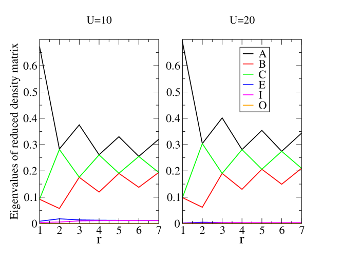
Figure 7: Eigenvalues of the reduced density matrix, $\rho_{2}$, for $U=10$ (left panel) and $U=20$ (right panel) as a function of distance $r$, for some eigenstates.

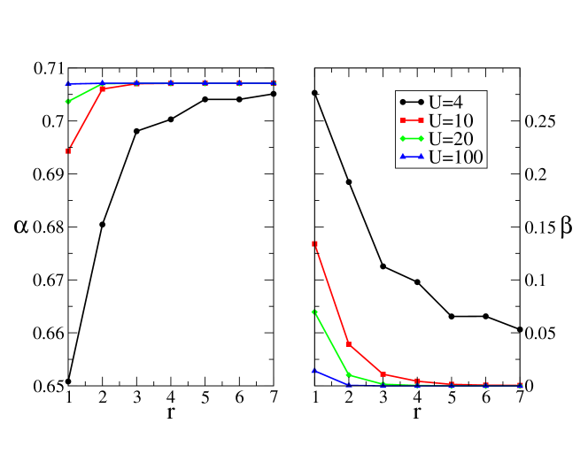
Figure 8: Relative weight of the spin up-spin - down-spin subspace $\alpha$ and doubly occupied-site - unoccupied-site subspace $\beta$ in the eigenstate with highest eigenvalue, $A$, for the matrix $\rho_{2}$.

States $B$ and $C$ (and its degenerate state $D$) also have a large weight. These states are spin triplets and antisymmetric in the space coordinates. Interestingly states where the spins at points $r=0$ and $r$ are parallel have equal or larger weight. For odd sites, states $B,C,D$ are degenerate but for even sites it is more favorable for the spins to be parallel. This is indicative of the long-range antiferromagnetic correlations in the large $U$ limit at half-filling.

States $E$ and $I$ are representative of mixtures between states involving singly occupied sites and doubly or unoccupied sites, either in antisymmetric or symmetric combinations, and have smaller weights.

Entanglement between doubly occupied sites and unoccupied sites enters indirectly via state $A$, since state $O$ has very low weight. The lowest probability state $P$ also has a mixture of the same four states, as well with a very small weight.

Even though the doubly occupied-site - unoccupied-site entanglement contributes to state $A$, the relative weight decreases fast with distance and interaction strength. This is illustrated in Fig. 8. In the left panel we show the relative weight of the spin up-spin - down-spin subspace $\alpha$ and in the right panel we show that of the doubly-occupied-site - unoccupied-site subspace $\beta$. Note that the dominant contribution comes from the spin up-spin - down-spin subspace $\alpha>\beta$. (As a side remark, the eigenstate with the lowest eigenvalue, $P$, has $\gamma<\delta$.) Comparing the various values of the interaction strength $U$, we see that $\beta$ decreases fast. The same happens as $r$ increases, which is consistent with the short range of the correlations between a doubly occupied site and a unoccupied site. For large $U$ the weight is mostly contained in the spin part, in a spin-singlet state. These results are consistent and clarify the previous results that the charge correlations are very short range, particularly as $U$ grows.

Tracing out all states except those with unoccupied or doubly occupied sites, we find a $4\times 4$ matrix that stores direct information on the correlations between a unoccupied site and a doubly occupied site. This density matrix may be defined as,

$$\rho_{3}=Tr^{\prime}\rho_{2}$$ (31)

where the trace is over the singly occupied sites.

The eigenstates of this reduced density matrix are of the form,

$$\begin{array}[]{ll}\mbox{eigenstate}&|\phi_{r=0};\phi_{r}\rangle=|n_{0,\uparrow}n_{r,\uparrow}n_{0,\downarrow}n_{r,\downarrow}\rangle\\ I&\frac{1}{\sqrt{2}}\left(|1010\rangle+|0101\rangle\right)\\ II&|1111\rangle\\ III&|0000\rangle\\ IV&\frac{1}{\sqrt{2}}\left(|1010\rangle-|0101\rangle\right)\end{array}$$

The results for the eigenvalues for $U=10,20$ of this reduced density matrix are shown in Fig. 9. The eigenvalue coresponding to state $I$ that mixes a doubly occupied site with a unoccupied site is the largest at small distances and as distance increases all states become equally probable. The decrease of the relative weight of state $I$ increases with $U$, consistent with previous results. This state is a $\eta$-spin triplet (note that this is consistent with the structure in Eq. 16). The lowest-weight state is a $\eta$-spin singlet. The degenerate states $II$ and $III$ correspond to two doubly occupied sites and two unoccupied sites.

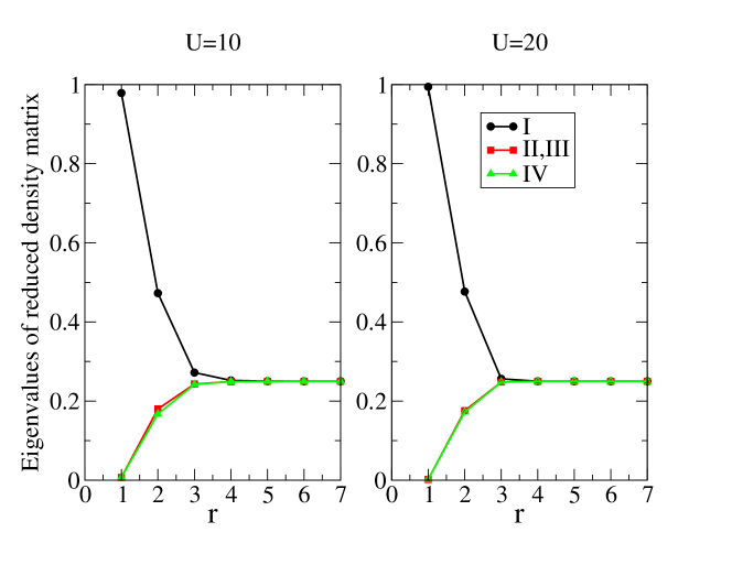
Figure 9: Eigenvalues of the reduced density matrix $\rho_{3}$ for $U=10$ (left panel) and $U=20$ (right panel), as a function of distance $r$.

For the subspace spanned by $\{|0>,|\uparrow,\downarrow>\}\times\{|0>,|\uparrow,\downarrow>\}$ defined on two sites, the entanglement can be measured by the concept of concurrence [29]. While the concurence is still a combination of some correlation functions, it is different from the traditional density-density or other types of correlation function. The entanglement results from the linear superposition principle of the quantum mechanics and is absent in the classical physics. Therefore, it is usually regarded as a kind of pure quantum correlation.

The reduced density matrix can be written as,

$$\rho_{3}=\left(\begin{array}[]{llll}u&0&0&0\\ 0&w_{1}&z&0\\ 0&z^{*}&w_{2}&0\\ 0&0&0&v\end{array}\right)$$ (32)

The concurrence, as the measure of the entanglement, can be calculated as,

$$C=2\mbox{max}[0,|z|-\sqrt{uv}]$$ (33)

The results for the concurrence show that both for $U=10$ and $U=20$ the correlations only extend to nearest-neighbors. The concurrence for higher values of the distance between the two sites $r>1$ vanishes. For nearest neighbors the concurrence takes the values $C=0.9577$ and $C=0.9884$ for $U=10$ and $U=20$, respectively, showing the large increase for large $U$ and that the correlation is strong, since the concurrence is close to $1$.

3 Summary

In this paper we have studied the correlation functions of basic entities of the one-dimensional Hubbard model using various methods. Previous analysis of the exact solution via the Bethe ansatz suggests the importance of correlations between doubly occupied and unoccupied sites and sites singly occupied with spin up and spin down electrons. These correlations have also been suggested by other treatments, as mentioned in the text.

The relevance of these operators is also stressed by their connection in terms of so-called rotated electrons with basic entities of the exact solution such as spinons and $\eta$-spinons. We have, therefore, calculated various correlation functions using an approximate mean-field solution within the Zou-Anderson transformation and with the introduction of non-local bond variables, in a way that is a reminder of the spinon and $\eta$-spinon bound and anti-bound states, respectively. Furthermore, we have used exact DMRG calculations of the same quantities and supplemented those with calculations of correlation functions for the operators introduced by Östlund and Granath, and further developed by one of the authors, which allow an exact charge-spin separation in a way that reminds the exact separation in low-dimensional systems.

We concluded that the charge-like correlation functions are typically very short ranged in the case of half filling, due to the charge gap. As the interaction strength increases, the correlations become virtually nearest-neighbor like. The spin-like correlation functions are however more extended in a way similar to the spin-spin correlation functions of the Hubbard model or, in the large $U$ limit, those of the spin-$1/2$ isotropic Heisenberg model. Even though the correlation functions calculated here are different from a standard longitudinal spin correlation function, their decay with distance is similar.

Further insight onto the correlations between two sites in a chain was obtained calculating the eigenvalues and eigenstates of the two-site reduced density matrix using exact diagonalization of a small system, also at half filling. The role of the spin and charge contributions to the entanglement between the two sites was clarified. As shown by the other methods, the correlations between doubly occupied sites and unoccupied sites are very short ranged, as evidenced by the concurrence which extends only to nearest neighbors. The eigenstates of the reduced density matrix corresponding to singly occupied sites with spin up or spin down have longer range.

The results using the mean-field approach were also extended to cases in the metallic phase (away from half-filling). The absence of the charge gap leads to correlations between a doubly occupied site and a unoccupied site that have larger range. The mean-field treatment also allows the study of higher energy phases. It was shown that for some of these phases the charge correlations have comparable ranges to those of the spin correlations.

Appendix A Mean-field solution using the Zou, Anderson transformation

Here we briefly review the mean-field solution of the Hubbard model in terms of the link variables introduced in Eq. (16). The bosonic and fermionic parts decouple. The mean-field Hamiltonian may be written as,

$$H_{MF}=H_{ed}+H_{SS}+C$$ (34)

where

$$H_{ed}= - t\sum_{i,\delta}\left\{\left(e_{i+\delta}^{\dagger}e_{i}-d_{i+\delta}^{\dagger}d_{i}\right)\left(\chi_{\delta,\uparrow}^{S}+\chi_{\delta,\downarrow}^{S}\right)+e_{i}d_{i+\delta}\Delta_{\delta}^{*}+d_{i}^{\dagger}e_{i+\delta}^{\dagger}\Delta_{\delta}\right\}$$ (35)

$$+ \sum_{i}d_{i}^{\dagger}d_{i}\left(U-\mu+\lambda_{i}\right)+\sum_{i}e_{i}^{\dagger}e_{i}\left(\mu+\lambda_{i}\right)$$

$$H_{SS}= - t\sum_{i,\delta}\left\{\left(\chi_{\delta}^{e}-\chi_{\delta}^{d}\right)\sum_{\sigma}S_{i,\sigma}^{\dagger}S_{i+\delta,\sigma}+\Phi_{\delta}\left(S_{i,\uparrow}^{\dagger}S_{i+\delta,\downarrow}^{\dagger}-S_{i,\downarrow}^{\dagger}S_{i+\delta,\uparrow}^{\dagger}\right)\right.$$ (36)

$$+ \left.\Phi_{\delta}^{*}\left(S_{i,\downarrow}S_{i+\delta,\uparrow}-S_{i,\uparrow}S_{i+\delta,\downarrow}\right)\right\}$$

$$+ \sum_{i,\sigma}\lambda_{i}S_{i,\sigma}^{\dagger}S_{i,\sigma}$$

$$C= t \sum_{i,\delta,\sigma}\left\{\left(\chi_{\delta}^{e}-\chi_{\delta}^{d}\right)\chi_{\delta,\sigma}^{S}+\Phi_{\delta}\Delta_{\delta}^{*}+\Phi_{\delta}^{*}\Delta_{\delta}\right\}$$ (37)

$$- \mu N-\sum_{i}\lambda_{i}$$

Defining the Fourier transforms of the operators as,

$$e_{r}=\frac{1}{\sqrt{N_{a}}}\sum_{k}e^{ikr}e_{k}$$ (38)

and

$$\chi_{k}^{A}=\sum_{\delta}e^{-ik\delta}\chi_{\delta}^{A}$$ (39)

where $A=e,d,S$, and similarly for $\Phi_{k}$ and $\Delta_{k}$, we can write in momentum space that,

$$H_{ed} = \sum_{k}\left\{\left(-t\sum_{\sigma}\chi_{k,\sigma}^{S}+\mu+\lambda_{0}\right)e_{k}^{\dagger}e_{k}+\left(t\sum_{\sigma}\chi_{k,\sigma}^{S}+U-\mu+\lambda_{0}\right)d_{k}^{\dagger}d_{k}\right.$$ (40)

$$+ \left.\left(-t\Delta_{k}^{*}e_{k}d_{-k}-t\Delta_{k}d_{k}^{\dagger}e_{-k}^{\dagger}\right)\right\}$$

That is,

$$H_{ed}=\sum_{k}\left\{E_{k}e_{k}^{\dagger}e_{k}+D_{k}d_{k}^{\dagger}d_{k}-t\Delta_{k}^{*}e_{k}d_{-k}-t\Delta_{k}d_{k}^{\dagger}e_{-k}^{\dagger}\right\}$$ (41)

where

$$E_{k} = -t\sum_{\sigma}\chi_{k,\sigma}^{S}+\mu+\lambda_{0}$$

$$D_{k} = t\sum_{\sigma}\chi_{k,\sigma}^{S}+U-\mu+\lambda_{0}$$

and

$$H_{SS} = \sum_{k}\left\{\sum_{\sigma}\left(-t(\chi_{k}^{e}-\chi_{k}^{d})+\lambda_{0}\right)S_{k,\sigma}^{\dagger}S_{k,\sigma}\right.$$ (42)

$$- t\left.\Phi_{k}\left(S_{k,\uparrow}^{\dagger}S_{-k,\downarrow}^{\dagger}-S_{k,\downarrow}^{\dagger}S_{-k,\uparrow}^{\dagger}\right)-t\Phi_{k}^{*}\left(S_{k,\downarrow}S_{-k,\uparrow}-S_{k,\uparrow}S_{-k,\downarrow}\right)\right\}$$

One then arrives to,

$$H_{SS} = \sum_{k,\sigma}\left\{\bar{\epsilon}_{k}S_{k,\sigma}^{\dagger}S_{k,\sigma}-t\Phi_{k}\left(S_{k,\uparrow}^{\dagger}S_{-k,\downarrow}^{\dagger}-S_{k,\downarrow}^{\dagger}S_{-k,\uparrow}^{\dagger}\right)\right.$$ (43)

$$- \left.t\Phi_{k}^{*}\left(S_{k,\downarrow}S_{-k,\uparrow}-S_{k,\uparrow}S_{-k,\downarrow}\right)\right\}$$

where

$$\bar{\epsilon}_{k}=-t(\chi_{k}^{e}-\chi_{k}^{d})+\lambda_{0}$$

We have assumed that the Lagrange multiplier is uniform and only the $k=0$ component is non-vanishing. For later purposes we define,

$$\gamma_{k}=\sum_{\delta}e^{-ik\cdot\delta}$$

We are left with the diagonalization of two quadratic Hamiltonians. This can be done in a standard way performing Bogoliubov-Valatin transformations. Defining,

$$e_{k} = u_{k}\alpha_{k}+v_{k}^{*}\beta_{-k}^{\dagger}$$

$$d_{-k} = u_{k}\beta_{-k}+v_{k}^{*}\alpha_{k}^{\dagger}$$ (44)

and similarly for the spin part,

$$s_{\uparrow,k} = \tilde{u}_{k}\tilde{\alpha}_{k}+\tilde{v}_{k}^{*}\tilde{\beta}_{-k}^{\dagger}$$

$$s_{\downarrow,-k} = \tilde{u}_{k}\tilde{\beta}_{-k}-\tilde{v}_{k}^{*}\tilde{\alpha}_{k}^{\dagger}$$ (45)

where $u_{k}^{2}-v_{k}^{2}=1$ for bosons and $\tilde{u}_{k}^{2}+\tilde{v}_{k}^{2}=1$ for fermions, and eliminating off-diagonal terms in the quasiparticle operators, we obtain that the diagonalized Hamiltonians take the forms,

$$H_{ed} = \sum_{k}\left\{\epsilon_{k}^{\alpha}\alpha_{k}^{\dagger}\alpha_{k}+\epsilon_{k}^{\beta}\beta_{-k}^{\dagger}\beta_{-k}+[\epsilon_{k}-1/2(E_{k}+D_{k})]\right\}$$

$$H_{SS} = \sum_{k}\left\{\tilde{\epsilon}_{k}\left(\tilde{\alpha}_{k}^{\dagger}\tilde{\alpha}_{k}+\tilde{\beta}_{-k}^{\dagger}\tilde{\beta}_{-k}\right)+[\bar{\epsilon}_{k}-\tilde{\epsilon}_{k}]\right\}$$ (46)

where

$$\epsilon_{k}^{\alpha} = \epsilon_{k}+1/2(E_{k}-D_{k})$$

$$\epsilon_{k}^{\beta} = \epsilon_{k}-1/2(E_{k}-D_{k})$$ (47)

with

$$\epsilon_{k}=\sqrt{\left(\frac{E_{k}+D_{k}}{2}\right)^{2}-t^{2}\Delta_{k}^{2}}$$ (48)

Note that $E_{k}+D_{k}=U+2\lambda_{0}$. Here,

$$\tilde{\epsilon}_{k}=\sqrt{\bar{\epsilon}_{k}^{2}+4t^{2}\Phi_{k}^{2}}$$ (49)

Also, we find that,

$$u_{k}v_{k} = \frac{t\Delta_{k}}{2\epsilon_{k}}$$

$$u_{k}^{2} = \frac{1}{2}\left\{\frac{E_{k}+D_{k}}{2\epsilon_{k}}+1\right\}$$

$$v_{k}^{2} = \frac{1}{2}\left\{\frac{E_{k}+D_{k}}{2\epsilon_{k}}-1\right\}$$ (50)

and

$$\tilde{u}_{k}\tilde{v}_{k} = \frac{t\Phi_{k}}{\tilde{\epsilon}_{k}}$$

$$\tilde{u}_{k}^{2} = \frac{1}{2}\left\{1+\frac{\bar{\epsilon}_{k}}{\tilde{\epsilon}_{k}}\right\}$$

$$\tilde{v}_{k}^{2} = \frac{1}{2}\left\{1-\frac{\bar{\epsilon}_{k}}{\tilde{\epsilon}_{k}}\right\}$$ (51)

The solution of the problem involves the self-consistent calculation of the averages appearing in these equations. Any average can now be calculated using the Bogoliubov-Valatin transformations.

The mean-field equations are given by,

$$\Delta_{k}=\frac{2}{N_{s}}\sum_{k^{\prime}}\gamma_{k-k^{\prime}}\left\{\tilde{u}_{k^{\prime}}\tilde{v}_{k^{\prime}}\left(1-2f(\tilde{\epsilon}_{k^{\prime}})\right)\right\}$$ (52)

$$\Phi_{k}=\frac{1}{N_{s}}\sum_{k^{\prime}}\gamma_{k-k^{\prime}}\left\{\right. + \left.u_{k^{\prime}}v_{k^{\prime}}\left(1+\delta_{k^{\prime},k_{\alpha}}N_{s}n_{\alpha}+(1-\delta_{k^{\prime},k_{\alpha}})f_{B}(\epsilon_{k^{\prime}}^{\alpha})\right)\right.$$ (53)

$$+ \left.u_{k^{\prime}}v_{k^{\prime}}\left(\delta_{k^{\prime},k_{\beta}}N_{s}n_{\beta}+(1-\delta_{k^{\prime},k_{\beta}})f_{B}(\epsilon_{k^{\prime}}^{\beta})\right)\right\}$$

$$\chi_{k,\sigma}^{S}=\frac{1}{N_{s}}\sum_{k^{\prime}}\gamma_{k-k^{\prime}}\left\{\tilde{u}_{k^{\prime}}^{2}f(\tilde{\epsilon}_{k^{\prime}})+\tilde{v}_{k^{\prime}}^{2}\left(1-f(\tilde{\epsilon}_{k^{\prime}})\right)\right\}$$ (54)

$$\chi_{k}^{e}=\frac{1}{N_{s}}\sum_{k^{\prime}}\gamma_{k-k^{\prime}}\left\{\right. + \left.u_{k^{\prime}}^{2}\left(\delta_{k^{\prime},k_{\alpha}}N_{s}n_{\alpha}+(1-\delta_{k^{\prime},k_{\alpha}})f_{B}(\epsilon_{k^{\prime}}^{\alpha})\right)\right.$$ (55)

$$+ \left.v_{k^{\prime}}^{2}\left(1+\delta_{k^{\prime},k_{\beta}}N_{s}n_{\beta}+(1-\delta_{k^{\prime},k_{\beta}})f_{B}(\epsilon_{k^{\prime}}^{\beta})\right)\right\}$$

$$\chi_{k}^{d}=\frac{1}{N_{s}}\sum_{k^{\prime}}\gamma_{k-k^{\prime}}\left\{\right. + \left.u_{k^{\prime}}^{2}\left(\delta_{k^{\prime},k_{\beta}}N_{s}n_{\beta}+(1-\delta_{k^{\prime},k_{\beta}})f_{B}(\epsilon_{k^{\prime}}^{\beta})\right)\right.$$ (56)

$$+ \left.v_{k^{\prime}}^{2}\left(1+\delta_{k^{\prime},k_{\alpha}}N_{s}n_{\alpha}+(1-\delta_{k^{\prime},k_{\alpha}})f_{B}(\epsilon_{k^{\prime}}^{\alpha})\right)\right\}$$

$$1=\frac{1}{N_{s}}\sum_{k}\left\{\right. + \left.u_{k}^{2}\left(\delta_{k,k_{\alpha}}N_{s}n_{\alpha}+(1-\delta_{k,k_{\alpha}})f_{B}(\epsilon_{k}^{\alpha})\right)\right.$$ (57)

$$+ \left.v_{k}^{2}\left(1+\delta_{k,k_{\beta}}N_{s}n_{\beta}+(1-\delta_{k,k_{\beta}})f_{B}(\epsilon_{k}^{\beta})\right)\right.$$

$$+ \left.u_{k}^{2}\left(\delta_{k,k_{\beta}}N_{s}n_{\beta}+(1-\delta_{k,k_{\beta}})f_{B}(\epsilon_{k}^{\beta})\right)\right.$$

$$+ \left.v_{k}^{2}\left(1+\delta_{k,k_{\alpha}}N_{s}n_{\alpha}+(1-\delta_{k,k_{\alpha}})f_{B}(\epsilon_{k}^{\alpha})\right)\right.$$

$$+ \left.2\tilde{u}_{k}^{2}f(\tilde{\epsilon}_{k})+2\tilde{v}_{k}^{2}\left(1-f(\tilde{\epsilon}_{k})\right)\right\}$$

$$n-1=-\left(n_{\alpha}+\sum_{k\neq k_{\alpha}}f_{B}(\epsilon_{k}^{\alpha})\right)+\left(n_{\beta}+\sum_{k\neq k_{\beta}}f_{B}(\epsilon_{k}^{\beta})\right)$$ (58)

where $f$ is the Fermi-Dirac distribution and $f_{B}$ the Bose-Einstein distribution.

The correlation functions may be calculated at the mean-field level. We obtain that,

$$C_{1}(r)=\frac{1}{N_{a}^{2}}\sum_{k_{1}}\sum_{k_{2}}$$ (59)

$$\left[|u_{k_{1}}|^{2}|u_{k_{2}}|^{2}+e^{-i(k_{1}-k_{2})r}u_{k_{1}}^{*}v_{k_{1}}u_{k_{2}}v_{k_{2}}^{*}\right]f_{B}(\epsilon_{k_{1}}^{\alpha})f_{B}(\epsilon_{k_{2}}^{\beta})$$

$$+ \left[|u_{k_{1}}|^{2}|v_{k_{2}}|^{2}+e^{-i(k_{1}-k_{2})r}u_{k_{1}}^{*}v_{k_{1}}u_{k_{2}}v_{k_{2}}^{*}\right]f_{B}(\epsilon_{k_{1}}^{\alpha})(1+f_{B}(\epsilon_{k_{2}}^{\alpha}))$$

$$+ \left[|v_{k_{1}}|^{2}|u_{k_{2}}|^{2}+e^{-i(k_{1}-k_{2})r}u_{k_{1}}^{*}v_{k_{1}}u_{k_{2}}v_{k_{2}}^{*}\right]f_{B}(\epsilon_{k_{2}}^{\beta})(1+f_{B}(\epsilon_{k_{1}}^{\beta}))$$

$$+ \left[|v_{k_{1}}|^{2}|v_{k_{2}}|^{2}+e^{-i(k_{1}-k_{2})r}u_{k_{1}}^{*}v_{k_{1}}u_{k_{2}}v_{k_{2}}^{*}\right](1+f_{B}(\epsilon_{k_{1}}^{\beta}))(1+f_{B}(\epsilon_{k_{2}}^{\alpha}))$$

and

$$\langle n_{e}(r)\rangle = \frac{1}{N_{a}}\sum_{k}\left[|u_{k}|^{2}f_{B}(\epsilon_{k}^{\alpha})+|v_{k}|^{2}(1+f_{B}(\epsilon_{k}^{\beta}))\right]$$

$$\langle n_{d}(r)\rangle = \frac{1}{N_{a}}\sum_{k}\left[|u_{k}|^{2}f_{B}(\epsilon_{k}^{\beta})+|v_{k}|^{2}(1+f_{B}(\epsilon_{k}^{\alpha}))\right]$$ (60)

Similarly,

$$C_{2}(r)=\frac{1}{N_{a}^{2}}\sum_{k_{1}}\sum_{k_{2}}$$ (61)

$$\left[|\tilde{u}_{k_{1}}|^{2}|\tilde{u}_{k_{2}}|^{2}+e^{i(k_{1}-k_{2})r}\tilde{u}_{k_{1}}^{*}\tilde{v}_{k_{1}}\tilde{u}_{k_{2}}\tilde{v}_{k_{2}}^{*}\right]f(\epsilon_{k_{1}}^{\beta})f(\epsilon_{k_{2}}^{\alpha})$$

$$+ \left[|\tilde{u}_{k_{1}}|^{2}|\tilde{v}_{k_{2}}|^{2}-e^{i(k_{1}-k_{2})r}\tilde{u}_{k_{1}}^{*}\tilde{v}_{k_{1}}\tilde{u}_{k_{2}}\tilde{v}_{k_{2}}^{*}\right]f(\epsilon_{k_{1}}^{\beta})(1-f(\epsilon_{k_{2}}^{\alpha}))$$

$$+ \left[|\tilde{v}_{k_{1}}|^{2}|\tilde{u}_{k_{2}}|^{2}-e^{i(k_{1}-k_{2})r}\tilde{u}_{k_{1}}^{*}\tilde{v}_{k_{1}}\tilde{u}_{k_{2}}\tilde{v}_{k_{2}}^{*}\right]f(\epsilon_{k_{2}}^{\alpha})(1-f(\epsilon_{k_{1}}^{\alpha}))$$

$$+ \left[|\tilde{v}_{k_{1}}|^{2}|\tilde{v}_{k_{2}}|^{2}+e^{i(k_{1}-k_{2})r}\tilde{u}_{k_{1}}^{*}\tilde{v}_{k_{1}}\tilde{u}_{k_{2}}\tilde{v}_{k_{2}}^{*}\right](1-f(\epsilon_{k_{1}}^{\alpha}))(1-f(\epsilon_{k_{2}}^{\beta}))$$

and

$$\langle n_{s,\uparrow}(r)\rangle = \frac{1}{N_{a}}\sum_{k}\left[|\tilde{u}_{k}|^{2}f(\epsilon_{k}^{\beta})+|\tilde{v}_{k}|^{2}(1-f(\epsilon_{k}^{\alpha}))\right]$$

$$\langle n_{s,\downarrow}(r)\rangle = \frac{1}{N_{a}}\sum_{k}\left[|\tilde{u}_{k}|^{2}f(\epsilon_{k}^{\alpha})+|\tilde{v}_{k}|^{2}(1-f(\epsilon_{k}^{\beta}))\right]$$ (62)

Appendix B DMRG method

In this Appendix a brief description of the DMRG method used in our studies is presented. The density matrix renormalization group (DMRG) [30] algorithm is an accurate method in dealing with quasi-one-dimensional system. It provides a criterion to find which states to keep and which to discard. Therefore, it can deal with relative large-size system with high accuracy. In the following, we give a brief introduction about this method and its application to our calculations.

In this method one constructs a superblock composed of the original system block and the environment block, usually the reflection of the system block. The reduced density matrix for the system block is defined as,

$$\rho_{ii^{\prime}}=\sum_{j}{\psi_{ij}^{*}\psi_{i^{\prime}j}}.$$ (63)

where $\psi$ is a state of the superblock. Usually it is chosen as the ground state corresponding to the zero temperature. Moreover, here $\left|i\right\rangle$ and $\left|j\right\rangle$ label the states of the system and the environment blocks, respectively. For any system block operator $A$, we have,

$$\left\langle A\right\rangle=\sum_{ii^{\prime}}A_{ii^{\prime}}\rho_{ii^{\prime}}=Tr\left(\rho A\right)=\Sigma_{\alpha}\omega_{\alpha}\left\langle u^{\alpha}\left|A\right|u^{\alpha}\right\rangle.$$ (64)

where ${\omega_{\alpha}}$ and $u^{\alpha}$ are the eigenvalues and eigenstates of the reduced matrix $\rho$. The significance of the state $u^{\alpha}$ can then be determined by $\omega_{\alpha}$. For a certain $\alpha$, if $\omega_{\alpha}$ is very small, its contribution to $\left\langle A\right\rangle$ is also very small. Then its corresponding state $u^{\alpha}$ can be discarded. Using this method, some states can be discarded during the growth of the system size and the size of the Hamilitonian of the system to be calculated is therefore reduced.

There are two basic DMRG algorithms—the infinite system and the finite system algorithms. For the infinite system case, the main process is as follows. We first choose a small-size system that can be exactly diagonalized, e.g. $L=4$ sites is taken in our calculations, as the superblock. Then use its ground state to form the reduced density matrix $\rho$ of the system block. The $m$ highest eigenvectors of $\rho$ are kept to renormalize the Hamilitonian of the system block $S$ and the corresponding operators. We add then two new sites and use these renormalized Hamiltonian and operators of $S$ to form a new superblock. By repeating these steps, the system size grows but the size of the Hamiltonian of the superblock keeps on a suitable size.

The finite-system case is based on the infinite system case by sweeping the superblock to reach a higher accuracy. For further detailes on the process, see Ref. [30].

In our DMRG calculations we have used the finite-system DMRG algorithm. Three sweeps have been taken to increase the accuracy. The numerical calculations were performed on finite chains, up to $100$ lattice sites, using the open boundary condition. Two sites were added in each step. For accuracy, the largest kept-state number reached $130$ and the truncation error is less than $10^{-7}$. To avoid the influence of the edge effect, the $r=0$ point was chosen in the middle of the chain.

References

References

- [1] J.M.P. Carmelo, arXiv:1211.5391; J.M.P. Carmelo and P.D. Sacramento, arXiv:1211.6073.
- [2] J.M.P. Carmelo, J. Román and K. Penc, Nucl. Phys. B 683, 387 (2004).
- [3] A. B. Harris and R. V. Lange, Phys. Rev. 157, 295 (1967).
- [4] J. Stein, J. Stat. Phys. 88, 487 (1997).
- [5] J.M.P. Carmelo, S. Östlund and M. J. Sampaio, Ann. Phys. 325, 1550 (2010).
- [6] A. H. MacDonald, S. M. Girvin and D. Yoshioka, Phys. Rev. B 37, 9753 (1988).
- [7] R.G. Leigh, P. Phillips and T.-P. Choy, Phys. Rev. Lett. 99, 046404 (2007).
- [8] T.-P. Choy, R.G. Leigh, P. Phillips and P.D. Powell, Phys. Rev. B 77, 014512 (2008).
- [9] P. Phillips, T.-P. Choy and R.G. Leigh, Rep. Prog. Phys. 72, 036501 (2009).
- [10] T.A. Kaplan, P. Horsch and P. Fulde, Phys. Rev. Lett. 49, 889 (1982).
- [11] A. Montorsi and M. Roncaglia, arXiv:1207.3426.
- [12] Z. Zou and P. W. Anderson, Phys. Rev. B 37, 627 (1988).
- [13] S. Östlund and M. Granath, Phys. Rev. Lett. 96, 066404 (2006).
- [14] I. Affleck, D. Gepner, H. J. Schulz, and T. Ziman, J. Phys. A 22, 511 (1989).
- [15] T. Giamarchi and H. J. Schulz, Phys. Rev. B 39, 4620 (1989).
- [16] R. R. P. Singh, M. E. Fisher, and R. Shankar, Phys. Rev. B 39, 2562 (1989).
- [17] K. A. Hallberg, P. Horsch, and G. Martínez, Phys. Rev. B 52, R719 (1995).
- [18] T. Hikihara and A. Furusaki, Phys. Rev. B 58, R583 (1998).
- [19] G. Kotliar and A.E. Ruckenstein, Phys. Rev. Lett. 57, 1362 (1986).
- [20] V. Dorin and P. Schlottmann, Phys. Rev. B 47, 5095 (1993).
- [21] P. Coleman, Phys. Rev. B 29, 3035 (1984).
- [22] R.G. Dias and J.M.B. Lopes dos Santos, J. Physique I 2, 1889 (1992).
- [23] N.M.R. Peres, R.G. Dias, P.D. Sacramento and J.M.P. Carmelo, Phys. Rev. B 61, 5169 (2000).
- [24] P. Ribeiro, P.D. Sacramento and M.A.N. Araújo, Ann. of Phys. 326, 1189 (2011).
- [25] P. A. Lee, N. Nagaosa and X.-G. Wen, Rev. Mod. Phys. 78, 17 (2006).
- [26] H. Shiba, Prog. Theor. Phys 48 , 2171 (1972); C. N. Yang and S. C. Zhang, Mod. Phys. Lett. B 4, 759 (1990); Shoucheng Zhang, Phys. Rev. Lett. 65, 120 (1990); V. J. Emery, Phys. Rev. B 14, 2989 (1976); A.B. Eriksson, T. Einarsson and S. Östlund, Phys. Rev. B 52 , 3662 (1995)
- [27] F.A. Berezin and M.S. Marinov, JETP Lett. 21, 320 (1975); Ann. Phys., N Y 104, 336 (1977); V.R. Vieira, Phys. Rev. B 23, 6043 (1981).
- [28] J.M.P. Carmelo, Nucl. Phys. B 824, 452 (2010).
- [29] W.K. Wootters, Phys. Rev. Lett. 80, 2245 (1998).
- [30] S. R White, et al., Density-Matrix Renormalization: A New Numerical Method in Physics, Springer, Berlin, (1999).