Properties of trapped neutrons interacting with realistic nuclear Hamiltonians

Abstract

We calculate properties of neutron drops in external potentials using both quantum Monte Carlo and no-core full configuration techniques. The properties of the external wells are varied to examine different density profiles. We compare neutron drop results given by a selection of nuclear Hamiltonians, including realistic two-body interactions as well as several three-body forces. We compute a range of properties for the neutron drops: ground-state energies, spin-orbit splittings, excitation energies, radial densities and rms radii. We compare the equations of state for neutron matter for several of these Hamiltonians. Our results can be used as benchmarks to test other many-body techniques, and to constrain properties of energy-density functionals.

I Introduction

There are three major motivations for investigating pure neutron systems with external fields (“neutron drops”) using ab initio approaches. First, neutron drops provide a very simple model of neutron-rich nuclei in which the core is approximated as an external well acting on valence neutrons Chang et al. (2004); Pieper (2005); Gandolfi et al. (2006, 2008). Second, ab initio solutions for neutrons trapped by an external potential can be used as data for calibrating model effective Hamiltonians and Energy Density Functionals (EDFs) Bogner et al. (2011); Gandolfi et al. (2011), particularly for very neutron-rich systems as occur in astrophysical environments like neutron stars. Third, these results may serve as useful benchmarks for testing other many-body methods.

These motivations are further supported by the advent of new experimental facilities to probe the extremes of neutron-rich nuclei, to map out the neutron drip line and to inform models of nuclear astrophysical processes Erler et al. (2012). Traditional energy density functionals Bender et al. (2003) are obtained by fitting measured properties of stable and near-stable nuclei. Extrapolations using these traditional EDFs to regions of extreme isospin are sensitive to their less controlled features that result in large variations in the predictions. Beyond these experimental vistas, we desire control over properties of EDFs for low-density neutron systems, since those properties are important for the processes in the inner crust of neutron stars. It is our long-term aim to provide ab initio calculations of trapped neutrons that address these motivations. We report here the results with currently available approaches that serve as a basis for long-term efforts that will employ improved microscopic Hamiltonians and many-body methods.

We adopt two nucleon-nucleon ($N\!N$) interactions which fit scattering data and deuteron properties with high accuracy, namely the local Argonne $v^{\prime}_{8}$ (AV8^′) Pudliner et al. (1997) and the nonlocal JISP16 Shirokov et al. (2007). As shown by accurate calculations Coon et al. (1979); Carlson et al. (1983); Chen et al. (1985); Pieper et al. (2001); Pudliner et al. (1997); Hayes et al. (2003); Navrátil et al. (2007); Maris et al. (2011); Roth et al. (2011), local $N\!N$ interactions are not sufficient to describe accurately the properties of light nuclei. Even the ground-state of the simplest three-body problem, the triton, is significantly underbound.

Different models of three-nucleon interactions (TNIs) have been proposed to build a non-relativistic Hamiltonian that reproduces experimental results such as ground-state energies, density profiles, and rms radii of light nuclei Pieper et al. (2001). TNIs from meson-exchange theory are modeled through an operator structure with parameters that are fit to experimental nuclear energies. The Urbana IX TNI (UIX) was fit to ³H and nuclear matter saturation, but it typically underbinds heavier nuclei Pudliner et al. (1997). Other TNI forms, namely Illinois forces, are fit to light nuclei Pieper et al. (2001). The most recent is the Illinois-7 (IL7) Pieper (2008) which reproduces nuclear energies up to $A=12$ with an rms error of 600 keV. However, the three-pion rings included in IL7 give a strong overbinding of pure neutron-matter Sarsa et al. (2003). In light of the different data selected for tuning these TNIs it is useful to observe their similarities and differences with neutron drops.

JISP16 is a phenomenological nonlocal $N\!N$-interaction written as a finite matrix in a harmonic oscillator (HO) basis for each of the $N\!N$ partial waves. It is constructed to reproduce the available $N\!N$ scattering data using the $J$-matrix inverse scattering approach. In addition, phase-equivalent transformations have been used to modify its off-shell properties in order to achieve a good description of selected states in light nuclei Shirokov et al. (2007). It gives a good description of most narrow states in light nuclei up to about $A=12$ Maris et al. (2009, 2010a); Cockrell et al. (2012). However it tends to overbind heavier $N=Z$ nuclei (¹⁶O is overbound by about 15%), but tends to underbind as one moves away from the valley of stability.

In this paper we analyze the ground-states and several excited states of neutron drops for four Hamiltonians: AV8^′ without TNI, AV8^′+UIX, AV8^′+IL7, and JISP16. We examine possible sub-shell closures and the spin-orbit splittings of odd systems near closed HO shells. We also compare results for the neutron matter equations of state using AV8^′ with and without TNIs that could be useful to calibrate bulk and gradient terms of Skyrme forces. The techniques we use are based on two quantum Monte Carlo (QMC) techniques for the Argonne interactions and on the No-Core Full Configuration (NCFC) for the nonlocal interaction JISP16. We provide quantified uncertainties where feasible.

The Green’s function Monte Carlo (GFMC) provides accurate energies, radii and and other properties of nuclei up to $A=12$ with the Argonne interactions Pieper (2008); currently it can be used for systems of up to 16 neutrons. The Auxiliary Field Diffusion Monte Carlo (AFDMC) Schmidt and Fantoni (1999) has similar statistical accuracy as GFMC in computing energies of systems of neutrons and can be implemented for larger systems, up to more than 100 neutrons Gandolfi et al. (2009a, 2011). A comparison between AFDMC and GFMC results (obtained with the same Hamiltonian) suggests that the systematic uncertainties are of the order of a few percent. Improving the trial wave function used in AFDMC to include pairing, for example, could further reduce these differences.

For JISP16 we expand the neutron drop wave functions in a HO basis. For any finite truncation of the basis, this provides us with a strict upper limit on the total energy of the system. Exact results are obtained by considering the limit of a complete (infinite-dimensional) HO basis — which we refer to as No-Core Full Configuration (NCFC) Maris et al. (2009). We can obtain the total energies for systems up to $A=14$ nucleons to within a percent by a simple extrapolation to the complete basis from a series of successive finite truncations. The extrapolation of other observables such as radii and densities is not as straightforward, but for small enough systems we can simply consider a large enough basis space in order to obtain converged results. Note that in a single run, at a fixed truncation, we not only obtain the ground state energy, but also the low-lying spectrum of the system.

The plan of the paper is the following: in Sec. II we describe various Hamiltonians we consider in this work. Then, in Sec. III we briefly review the different Monte Carlo many-body techniques used to solve for the neutron drops. Sec. IV presents an overview of the NCFC approach and Sec. V presents our main results for finite neutron drops. We present our results for neutron matter in Sec. VI and our conclusions in Sec. VII.

II Hamiltonians

We adopt non-relativistic Hamiltonians with the following general form:

$$H=-\sum_{i}{\hbar^{2}\over 2m}\nabla_{i}^{2}+\sum_{i}U_{\hbox{\scriptsize ext}}(r_{i})+\sum_{i<j}v_{ij}+\sum_{i<j<k}V_{ijk}\,.$$ (1)

Systems consisting of only neutrons are not expected to be self-bound. Therefore it is necessary to include an external well $U_{\hbox{\scriptsize ext}}(r)$ in the Hamiltonian to have a confined system. We consider both harmonic oscillator (HO) wells and a Woods-Saxon (WS) potential.

The HO wells have the form

$$U_{HO}(r)=\frac{1}{2}m\Omega^{2}r^{2}\,.$$ (2)

This potential is useful due to its simplicity and the fact that the ground state may be driven to arbitrary low density (i.e. with arbitrarily weak external harmonic potential strength) or arbitrarily large particle number. The convergence of both the Monte Carlo and the configuration interaction methods are improved due to the lack of any low-lying states with long-range tails in the wave function. This feature enables applying our results for tests of EDFs over a range from moderately low to rather high densities. Most of our results are for HO wells. Woods-Saxon wells have been used in other calculations of properties of neutron drops. In particular neutron drops with a WS well and the Argonne $v_{18}$ $N\!N$ and Illinois-2 potentials have been shown to provide a good description of oxygen isotopes Pieper (2005). The WS form is

$$U_{WS}(r)=\frac{U_{0}}{1+e^{(r-R)/a}}\,,$$ (3)

where we have used $a=1.1$ fm, $U_{0}=-35.5$ MeV and $R=3$ fm, that is, the same parameters as in Ref. Chang et al. (2004).

In addition to the total energy, $E=\langle H\rangle$, we also calculate other observables, such as the external energy $\langle U_{\hbox{\scriptsize ext}}\rangle$, the internal energy $E_{\hbox{\scriptsize int}}=\langle H\rangle-\langle U_{\hbox{\scriptsize ext}}\rangle$, and the rms radius $r$. Note that for a HO well, the external energy $\langle U_{\hbox{\scriptsize ext}}\rangle$ is proportional to $r^{2}$, and thus the quantities $E$, $E_{\hbox{\scriptsize int}}$, and $r$ are not independent observables in a HO well; however, in a WS well they are independent.

II.1 Argonne $N\!N$ interaction and three-body forces

One of the $N\!N$ potentials we adopt here is the Argonne AV8^′ Pudliner et al. (1997); Wiringa and Pieper (2002). It is a simplified version of the Argonne AV18 Wiringa et al. (1995), with the advantage that it can be exactly included in both GFMC and AFDMC algorithms without treating any part perturbatively. Other non-local operators appearing in AV18 must be included as a perturbation of AV8^′ in QMC calculations Pudliner et al. (1997). These perturbative corrections can be accurately computed within GFMC, but not in AFDMC. Thus we consider AV8^′ to facilitate comparisons of the two different QMC methods. The difference between the binding energies from AV8^′ and AV18 is very small in light nuclei, and much smaller in pure neutron systems; about 0.06 MeV per neutron Pieper et al. (2001).

The Argonne AV8^′ is a sum of eight operators:

$$v_{ij}=\sum_{p}v_{p}(r_{ij})O_{ij}^{p}$$ (4)

in which the $v_{p}(r_{ij})$ depend on the distance between the nucleons $i$ and $j$, and $O_{ij}^{p}$ are operators. Their form is

$$O_{ij}^{p=1,8}=(1,\vec{\sigma}_{i}\cdot\vec{\sigma}_{j},S_{ij},\vec{L}_{ij}\cdot\vec{S}_{ij})\times(1,\vec{\tau}_{i}\cdot\vec{\tau}_{j})$$ (5)

with $S_{ij}$ the tensor operator, $\vec{L}_{ij}$ the relative angular momentum and $\vec{S}_{ij}$ the total spin. The $v_{p}(r)$ parts are fit to reproduce the S and P partial waves as well as the ${}^{3}D_{1}$ wave and its coupling to ${}^{3}S_{1}$ of the full AV18 potential Wiringa et al. (1995).

In this paper we consider the AV8^′ alone and combined with two different three-body forces: the Urbana-IX (UIX) Pudliner et al. (1995) and the Illinois-7 (IL7) Pieper (2008). Just like for the $N\!N$ interaction, the TNIs are sums of several operators:

$$V_{ijk} = A_{2\pi}^{PW}O^{2\pi,PW}_{ijk}+A_{2\pi}^{SW}O^{2\pi,SW}_{ijk}+A_{3\pi}^{\Delta R}O^{3\pi,\Delta R}_{ijk}$$ (6)

$${}+A_{R}O^{R}_{ijk}+A_{R}^{T=3/2}O^{R,T=3/2}_{ijk}\,.$$

Both TNIs include the Fujita-Miyazawa operator $O^{2\pi,PW}$ and a phenomenological part $O^{R}$, while only IL7 has the $O^{2\pi,SW}_{ijk}$ ,$O^{3\pi,\Delta R}_{ijk}$, and $O^{R,T=3/2}_{ijk}$ terms. In the Fujita-Miyazawa term Fujita and Miyazawa (1957) two pions are exchanged between the three nucleons with the creation of an intermediate excited state. The phenomenological part $O^{R}$ has no spin or isospin dependence. The additional IL7 terms involve exchanges of two or three pions and a pure $T=3/2$ repulsion. A full description of the operators is given in Refs. Pieper et al. (2001); Pieper (2008).

The $A_{2\pi}^{PW}$ and $A_{R}$ parameters of UIX are determined by reproducing the binding energy of ³H and nuclear matter Pudliner et al. (1995). The UIX model has been used to investigate properties of neutron matter (see for example Refs. Akmal et al. (1998); Gandolfi et al. (2009a, 2012) and references therein). The resulting equation of state will support neutron stars larger than two solar masses.

The Illinois forces are more sophisticated than UIX. The $A$ coefficients are determined by fits to binding energies of light nuclei Pieper et al. (2001); Pieper (2008). The Illinois forces give a good description of properties of nuclei up to $A=12$, including both ground states and excited states, however three-pion operators are very attractive in pure neutron systems and they overbind neutron matter at large densities Sarsa et al. (2003). In this work, we consider IL7 as described in Pieper (2008).

II.2 JISP16

The JISP16 $N\!N$ interaction is determined by inverse scattering techniques from the $np$ phase shifts and is, therefore, charge symmetric. JISP16 is available in a relative HO basis Shirokov et al. (2007) and can be written as a sum over partial waves

$${\hat{V}}=\sum_{S,{\cal J},T}{\cal P}_{S,{\cal J},T}\sum_{n,\ell,n^{\prime},\ell^{\prime}}\;|nl\rangle\ A^{S,{\cal J},T}_{n\ell,n^{\prime}\ell^{\prime}}\ \langle n^{\prime}\ell^{\prime}|$$ (7)

where $\hbar\Omega=40$ MeV and ${\vec{\cal J}}={\vec{\ell}}+{\vec{s}}$. The HO relative coordinate wave function is written $\langle r|n\ell\rangle={\cal R}_{n\ell}(r)$. A small number of coefficients $\{A^{S,{\cal J},T}_{n\ell,n^{\prime}\ell^{\prime}}\}$ are sufficient to describe the phase shifts in each partial wave. Note that the JISP16 interaction is non-local and its off-shell properties have been tuned by phase-shift equivalent transformations to produce good properties of light nuclei. For example, JISP16 is tuned in the ${}^{3}S_{1}-^{3}D_{1}$ channel to give a high precision description of the deuteron’s properties. Other channels are tuned to provide good descriptions of ³H binding, the low-lying spectra of ⁶Li and the binding energy of ¹⁶O Shirokov et al. (2007). After its initial introduction, it was realized that the ¹⁶O energy was not fully converged and JISP16 overbinds ¹⁶O by about 15 to 20 MeV Maris et al. (2009). With these off-shell tunings to nuclei with $A\geq 3$ one may view JISP16 as simulating, to some approximation, what would appear as $N\!N\!N$ interaction contributions (as well as higher-body interactions) in alternative formulations of the nuclear Hamiltonian.

III Quantum Monte Carlo methods

Both of our QMC methods use diffusion Monte Carlo to project the lowest-energy eigenstate out of a trial wave function $\Psi_{T}$ by a propagation in imaginary time $\tau$:

$$\Psi(\tau)=e^{-(H-E_{T})\tau}\Psi_{T}\,,$$ (8)

where $E_{T}$ is a normalization factor. In the $\tau\rightarrow\infty$ limit the only component of $\Psi_{T}$ that survives is the lowest-energy one not orthogonal to $\Psi_{T}$:

$$\Psi_{0}=\lim_{\tau\rightarrow\infty}\Psi(\tau)\,.$$ (9)

The evolution in imaginary time is performed by using Monte Carlo integration to evaluate

$$\Psi(R,\tau)=\int dR^{\prime}G(R,R^{\prime},\tau)\Psi_{T}(R^{\prime})\,,$$ (10)

where $G(R,R^{\prime},\tau)$ is an approximation of the many-body Green’s function of the Hamiltonian, and $R$ and $R^{\prime}$ are the positions of all $A$ nucleons: $R\equiv(\vec{r}_{1},\dots,\vec{r}_{N})$. The exact form of $G(R,R^{\prime},\tau)$ is unknown, but it can be accurately approximated as a product of many $G(R,R^{\prime},\Delta\tau)$ for a small time step, $\Delta\tau$. The main difference between GFMC and AFDMC is in their representations of $\Psi$ and the structure of the initial $\Psi_{T}$.

III.1 GFMC method and trial wavefunction

GFMC uses a complete spin-isospin representation of the many-body wave function; $\Psi(R,\tau)$ is written as a vector with $2^{A}N(T)$ complex components. Here the $2^{A}$ allows for all possible nucleon spin up or down combinations and $N(T)$ is the number of proton-neutron combinations with the desired isospin. In the case of neutron drops $N(T)=1$. The exponential growth of the vector size with the number of neutrons currently limits GFMC calulations of neutron systems to $N\leq 16$.

Calculations of nuclei with realistic interactions face a sign problem eventually as the trial wave function is propagated to large $\tau$. To deal with this problem, we use the constrained path algorithm to obtain configurations with the largest possible overlap with the ground state Wiringa et al. (2000). This method is similar to the fixed node approximation in that it is exact in the limit of an exact constraint, and it is stable to large imaginary time; however it does not provide an upper bound. We then extend the propagation without constraint for as long as possible to obtain the energy and ground-state properties. The constraint and the convergence properties of GFMC are discussed in Wiringa et al. (2000), Figure 3 in that paper shows some convergence results for neutron drops.

The trial wave functions used in our GFMC calculations for neutron drops in HO wells are somewhat simplified from the ones described in Ref. Pudliner et al. (1997) for nuclei:

$$|\Psi_{T}\rangle = \left[{\cal S}\prod_{i<j}(1+U_{ij})\right]|\Psi_{J}\rangle\ ,$$ (11)

$$|\Psi_{J}\rangle = \left[\prod_{i<j}f_{c}(r_{ij})\right]|\Phi_{N}(JMTT_{3})\rangle\ .$$ (12)

The non-central $U_{ij}$ and associated central $f_{c}$ are optimal correlations for neutron matter of the form described in Ref. Pieper et al. (1992). For drops with $N\leq 8$, the $\Phi_{N}$ is expanded in an $LS$ basis of $s$- and $p$-shell oscillator functions as described in Ref. Pudliner et al. (1997). For $N\geq 8$ we use a “BCS” ansatz $\Phi_{\hbox{\scriptsize BCS}}$ of the form introduced in Refs. Carlson et al. (2003); Chang et al. (2004). For $N=8$ the two forms give very similar variational energies.

The BCS pairing is important, particularly for low-density systems and when trying to calculate even-odd staggering of the energies. In this paper we consider $\Phi_{\hbox{\scriptsize BCS}}$ for only $J=0$ states or, in the case of odd $N$, for states in which the total $J$ is carried by a single neutron. Such $\Phi_{\hbox{\scriptsize BCS}}$ are written using correlated pairs of neutrons with total spin $S=0$ and a $L=0$ spatial wave function $\phi_{ij}$ expanded in 0$s$, 0$p$, 1$s$, and 0$d$ single-neutron wave functions:

$$\phi_{ij} = \beta_{0s}\phi_{0s}(r_{i})\phi_{0s}(r_{j})+\beta_{0p}\phi_{0p}(r_{i})\phi_{0p}(r_{j})P_{1}(\hat{r}_{ij})$$ (13)

$${}+\beta_{1s}\phi_{1s}(r_{i})\phi_{1s}(r_{j})$$

$${}+\beta_{0d}\phi_{0d}(r_{i})\phi_{0d}(r_{j})P_{2}(\hat{r}_{ij})\ .$$

The $\beta_{nl}$ are variational parameters; only their ratios are relavant. For even $N$,

$$\Phi_{\hbox{\scriptsize BCS}}(J=0)=\sum_{P}|\phi_{ij}|~{}~{}|s_{1}s_{2}\cdots s_{N}\rangle\ ,$$ (14)

where the sum is over all partitions of $N$ neutrons into $N/2$ spin-up neutrons and $N/2$ spin-down neutrons, $i$ is from the set of spin-up neutrons and $j$ is from the set of spin-down neutrons, $|\phi_{ij}|$ is a determinant, and $|s_{1}s_{2}\cdots s_{N}\rangle$ is the spin-vector component with the given spins. For odd $N$ and $s_{1/2}$ or $d_{5/2}$ states we have

$$\Phi_{\hbox{\scriptsize BCS}}(M\!=\!J)={\cal A}\left[\phi_{L,S,J,M}({\bf r}_{N},\sigma_{N})\ \Phi_{\hbox{\scriptsize BCS,N-1}}(J\!=0\!)\right]\ ,$$ (15)

which is also a sum over partitions of determinants.

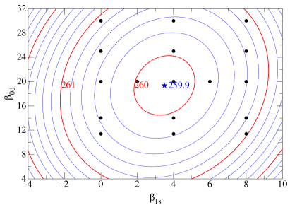
Figure 1: (color online) Contours of VMC energies for 12 neutrons in a 10-MeV HO well with AV8^′+UIX versus the 0$d$ and 1$s$ coefficients in the BCS wave function. The dots show the cases that were computed using GFMC.

Figure 1 shows the variational Monte Carlo (VMC) energies computed for systems of 12 neutrons with different BCS parameters for the 0$d$ and 1$s$ pairs; the $\beta_{0s}$ and $\beta_{0p}$ are fixed at 100 each so the ⁸n core is almost full. The optimized choice is used for the GFMC calculations. The total VMC or GFMC energy is not very sensitive to the choice of parameters (the contour interval is only 0.08%) - the effects on pairing can be larger. A detailed description of the algorithm as well as the importance sampling technique (constrained propagation) used to reduce the variance can be found in Refs. Pudliner et al. (1997); Wiringa et al. (2000).

The VMC energies computed with $\Psi_{T}$ or even just $\Psi_{J}$ are much closer to the final GFMC energies than is the case for real nuclei. The values using $\Psi_{J}$ are typically less than 10% above the GFMC values and often display better convergence as the number of unconstrained steps (see Ref. Wiringa et al. (2000)) is increased.

III.2 GFMC numerical convergence and error estimate

QMC calculations have an easily quantified statistical error arising from the Monte Carlo method. It is not so straightforward to determine the magnitude of the systematic errors arising from approximations made in the constrained-path implementation. These have been extensively discussed for GFMC in Refs. Pudliner et al. (1997); Wiringa et al. (2000).

Quantities other than the energy are usually evaluated by combining mixed and variational estimates:

$$\langle\Psi_{0}|{\cal O}|\Psi_{0}\rangle=2\langle\Psi_{0}|{\cal O}|\Psi_{T}\rangle-\langle\Psi_{T}|{\cal O}|\Psi_{T}\rangle.$$ (16)

No extrapolation for the energy is required since the ground state is an eigenstate of the Hamiltonian and the propagation commutes with the Hamiltonian. This linear extrapolation is usually very accurate if the calculation begins with a good trial wave function. It is also possible to estimate other observables by forward walking techniques or by adding a small perturbation $\epsilon{\cal O}$ to the Hamiltonian and computing the difference between the energy of the original and perturbed Hamiltonian. We have not pursued these methods for the present paper. Hence the internal energy results as well as other quantities reported below are extrapolated and potentially not as accurate as the full energy.

III.3 AFDMC method and trial wave function

The presence of spin operators in the Hamiltonian requires a summation of all possible good spin states in the wave function. In AFDMC the spin states are sampled using Monte Carlo techniques Schmidt and Fantoni (1999). This sampling is performed by reducing the quadratic dependence of spin operators in the exponential of Eq. (8) to a linear form by means of a Hubbard-Stratonovich transformation. The effect of an exponential of a linear combination of spin operators consists of a rotation of the spinor for each neutron during the propagation, and this permits the use of a much simpler basis in the trial wave function. The result is that the wave function is less accurate, but it can be rapidly evaluated. Since both positions and spins can be sampled, the AFDMC method can be used to solve for the ground state of much larger systems than GFMC – more than one-hundred neutrons currently may be solved with AFDMC.

More detailed explanations of the AFDMC method and how to include the full $N\!N$ interactions and TNIs in the propagator can be found in Refs. Sarsa et al. (2003); Pederiva et al. (2004); Gandolfi et al. (2009a), where the constrained-path approximation used to control the fermion sign problem is also discussed.

The AFDMC method projects out the lowest energy state with the same symmetry as the trial wave function from which the projection is started. The trial wave function used in the AFDMC algorithm has the form:

$$|\Psi_{T}(R,S)\rangle=\left[\prod_{i<j}f(r_{ij})\right]|\Phi_{JM}(R,S)\rangle\,,$$ (17)

where $S\equiv(s_{1},\dots,s_{N})$. The spin assignments $s_{i}$ consist in giving the spinor components, namely

$$s_{i}\equiv\left(\begin{array}[]{c}u_{i}\\ d_{i}\end{array}\right)=u_{i}|\uparrow\rangle+d_{i}|\downarrow\rangle\ ,$$ (18)

where $u_{i}$ and $d_{i}$ are complex numbers. The Jastrow function $f(r)$ is the solution of a Schrödinger-like equation for $f(r<d)$,

$$-\frac{\hbar^{2}}{m}\nabla^{2}f(r)+\alpha v_{c}(r)f(r)=\lambda f(r)\,,$$ (19)

where $v_{c}(r)$ is the spin-independent part of the nucleon-nucleon interaction, and the healing distance $d$ and $\alpha$ are variational parameters. For distances $r\geq d$ we impose $f(r)=1$. The Jastrow part of the function in our case has the only role of reducing the overlap of nucleons, therefore reducing the energy variance.

The antisymmetric part of the wave function is

$$\Phi_{JM}(R,S)=\Big{[}\sum D\{\phi_{\alpha}(\vec{r}_{i},s_{i})\}\Big{]}_{J,M}\,,$$ (20)

where $\alpha=\{n,l,j,m_{j}\}$ is the set of quantum numbers of single-particle orbitals, and the summation of determinants gives a trial wave function that is an eigenstate of $J^{2}$ and $M$. The single-particle basis is given by

$$\phi_{\alpha}(\vec{r}_{i},s_{i})=\Phi_{nlj}(r_{i})\left[Y_{l,m_{l}}(\hat{r}_{i})\xi_{s,m_{s}}(s_{i})\right]_{j,m_{j}}\,.$$ (21)

The radial components $\Phi_{nlj}$ are obtained by solving the Hartree–Fock problem with the Skyrme force SKM Pethick et al. (1995), $Y_{l,m_{l}}$ are spherical harmonics, and $\xi_{s,m_{s}}$ are spinors in the usual up-down basis. For each $(J,M)$ set of quantum numbers there are several combinations of single-particle orbitals. We typically perform several simulations to identify the ground-state and order of excited states. It is also possible to include a BCS pairing term in the trial wave function in AFDMC, as has been done for GFMC. This would allow more accurate treatment of pairing in very low-density systems, and is currently under development.

For neutron matter calculations we change the antisymmetric part of the wave function to be the ground state of the Fermi gas, built from a set of plane waves. The infinite uniform system is simulated by a cubic periodic box of volume $L^{3}$ according to the density of the system. The momentum vectors in this box are

$$\mathbb{k}_{\alpha}=\frac{2\pi}{L}(n_{\alpha x},n_{\alpha y},n_{\alpha z})\,,$$ (22)

where $\alpha$ labels the quantum state and $n_{x}$, $n_{y}$ and $n_{z}$ are integer numbers describing the state. The single-particle orbitals are given by

$$\phi_{\alpha}(\vec{r},s)=e^{i\vec{k}_{\alpha}\cdot\vec{r}}\xi_{s,m_{s},\alpha}(s)\,.$$ (23)

Again, it is possible to generalize the neutron matter calculations to include BCS pairing in the trial state Gandolfi et al. (2008, 2009b).

III.4 AFDMC numerical convergence and error estimate

AFDMC is very similar in concept to GFMC and convergence and error estimates are also similar. The statistical errors are easily evaluated and controllable. AFDMC also uses a constrained-path method to circumvent the fermion sign problem, and hence the results depend to some degree on the choice of trial function.

Although it is possible to do some unconstrained propagation with AFDMC, it is more limited than GFMC because the sampling of the spins introduces a fermion sign problem earlier. Uncertainties can also be addressed by choosing several different initial trial states. We find the constrained path results to be reasonably accurate when compared with GFMC for small systems.

		GFMC	AFDMC	Difference
		(MeV)	(MeV)	(MeV)	%
$N$	$J^{\pi}$	5 MeV HO well
8	0+	$67.00(1)$	$67.1(1)$	$0.1(1)$	$0.1$
9	$\frac{1}{2}^{+}$	$80.90(4)$	$81.2(1)$	$0.3(1)$	$0.4$
9	$\frac{5}{2}^{+}$	$81.20(3)$	$81.9(1)$	$0.7(1)$	$0.9$
10	0+	$92.1(1)$	$94.6(1)$	$2.5(2)$	$2.7$
11	$\frac{5}{2}^{+}$	$106.3(1)$	$108.0(1)$	$1.7(2)$	$1.6$
11	$\frac{1}{2}^{+}$	$105.9(1)$	$108.4(1)$	$2.5(2)$	$2.3$
12	0+	$118.1(1)$	$121.1(1)$	$3.0(2)$	$2.5$
13	$\frac{5}{2}^{+}$	$131.5(1)$	$135.7(2)$	$4.2(3)$	$3.1$
13	$\frac{1}{2}^{+}$	$130.8(1)$	$134.1(2)$	$3.3(3)$	$2.5$
14	0+	$142.2(2)$	$146.7(1)$	$4.5(3)$	$3.1$
$N$	$J^{\pi}$	10 MeV HO well
3	$\frac{3}{2}^{-}$	$45.5(0)$	$45.0(1)$	$-0.5(1)$	$-1.1$
3	$\frac{1}{2}^{-}$	$46.70(1)$	$46.7(1)$	$0.0(1)$	$0.0$
4	0+	$62.00(1)$	$62.9(1)$	$0.9(1)$	$1.4$
5	$\frac{3}{2}^{-}$	$83.00(1)$	$82.9(1)$	$-0.1(1)$	$-0.1$
5	$\frac{1}{2}^{-}$	$84.00(2)$	$83.7(1)$	$-0.3(1)$	$-0.3$
6	0+	$98.90(2)$	$98.4(1)$	$-0.5(1)$	$-0.5$
7	$\frac{1}{2}^{-}$	$118.9(0)$	$118.0(1)$	$-0.9(1)$	$-0.7$
7	$\frac{3}{2}^{-}$	$121.1(0)$	$120.6(1)$	$-0.5(1)$	$-0.4$
8	0+	$135.8(0)$	$134.7(1)$	$-1.1(1)$	$-0.8$
9	$\frac{1}{2}^{+}$	$163.7(1)$	$163.5(1)$	$-0.2(2)$	$-0.1$
9	$\frac{5}{2}^{+}$	$163.2(1)$	$162.5(1)$	$-0.7(2)$	$-0.4$
10	0+	$188.1(6)$	$188.5(1)$	$0.4(7)$	$0.2$
11	$\frac{5}{2}^{+}$	$217.0(3)$	$216.7(1)$	$-0.3(4)$	$-0.1$
11	$\frac{1}{2}^{+}$	$216.1(3)$	$216.6(2)$	$0.5(5)$	$0.2$
12	0+	$242.0(6)$	$240.8(1)$	$-1.2(7)$	$-0.5$
13	$\frac{5}{2}^{+}$	$267.6(6)$	$266.3(2)$	$-1.3(8)$	$-0.5$
13	$\frac{1}{2}^{+}$	$268.0(5)$	$267.2(2)$	$-0.8(7)$	$-0.3$
14	0+	$291.9(2)$	$291.2(2)$	$-0.7(4)$	$-0.2$

Table 1: Comparison of GFMC and AFDMC total energies for neutron drops in 5 MeV and 10 MeV wells with AV8^′+UIX. Statistical errors due to the Monte Carlo sampling are given in brackets.

In Table 1 we compare the GFMC and AFDMC total energy results for neutron drops in 5 and 10 MeV HO wells. Overall the agreement is of the order of a few percent or better. Statistical errors due to sampling can be made arbitrarily small, these are about 0.2% or less for the AFDMC and GFMC calculations.

For the lower densities generated by the 5 MeV well the GFMC energies are significantly lower than the AFDMC energies, by up to 3%. A plausible explanation for these discrepancies is the fact that we have not incorporated BCS pairing in the AFDMC calculation. Indeed, the differences are nearly zero for the closed shell at $N=8$ (where pairing does not play a role) and grow as we go towards the middle of the shell, $N=14$. We are therefore pursuing the inclusion of BCS pairing in the AFDMC calculations of neutron drops in order to improve the results at low densities. On the other hand, for the 10 MeV well the GFMC and AFDMC results are all within 1% of each other, with the AFDMC typically lower than the GFMC energies.

Systematic errors in calculations of neutron matter are similar in spirit. The trial wave function can affect results for the energy at low densities where pairing is important. At larger densities, though, pairing provides a very small fraction of the total energy of the system and calculations are much less sensitive to the choice of the trial state.

In addition to the Monte Carlo errors and the dependence on the choice of the trial state, we have to consider finite-size effects for calculations of neutron matter. We enforce periodic boundary conditions and fix the number of neutrons to be a closed shell in the periodic free-particle basis. In order to reduce finite-size effects we performed simulations with 66 neutrons. Free fermions for $N=66$ provide a kinetic energy very close to the infinite limit. Any possible finite-size effect due to the truncation of the potential energy is properly taken into account by considering several replicas of the simulation box as described in Ref. Sarsa et al. (2003); Gandolfi et al. (2009a). Typically these uncertainties are very small for bulk properties like the ground-state energy.

IV No Core Full Configuration method

The NCFC method is based on a series of no-core configuration interaction calculations with increasing basis dimensions. In this approach the wave function for the $N$ neutrons is expanded in an $N$-body basis of Slater determinants of single-particle states, and the many-body Schrödinger equation becomes a large sparse matrix eigenvalue problem. We obtain the lowest eigenstates of this matrix iteratively. In a complete basis, this method would give exact results for a given input interaction $V$. However, practical calculations can only be done in a finite-dimensional truncation of a complete basis. We perform a series of calculations until we reach numerical convergence in a sufficiently large basis space, or we employ a simple extrapolation Maris et al. (2009) to the complete basis.

IV.1 Description of basis space

Our choice for the basis is the harmonic oscillator (HO) basis so there are two basis space parameters, the HO energy $\hbar\omega$ and the many-body basis space cutoff $N_{\hbox{\scriptsize max}}$. The cutoff parameter $N_{\hbox{\scriptsize max}}$ is defined as the maximum number of total oscillator quanta allowed in the many-body basis space above the minimum for that number of neutrons. Numerical convergence is defined as independence of both basis space parameters $N_{\hbox{\scriptsize max}}$ and $\hbar\omega$, within evaluated uncertainties. Note that the basis space parameter $\hbar\omega$ is not necessarily the same as that of the HO well $\hbar\Omega$ that confines the neutrons.

We employ a many-body basis in the so-called $M$-scheme: the many-body basis states are Slater determinants in a HO basis, limited by the imposed symmetries — parity and total angular momentum projection ($M$), as well as by $N_{\hbox{\scriptsize max}}$. Each single-particle HO state has its orbital and spin angular momenta coupled to good total angular momentum, $j$, and magnetic projection, $m$. Here we only consider natural-parity states, and utilize $M=0$ for an even number of neutrons, and $M=\frac{1}{2}$ for an odd number of neutrons. In this scheme a single calculation gives the entire spectrum for that parity and $N_{\hbox{\scriptsize max}}$.

The NCFC approach satisfies the variational principle and guarantees uniform convergence from above to the exact eigenvalue with increasing $N_{\hbox{\scriptsize max}}$. That is, the results for the energy of the lowest state of each spin and parity, at any $N_{\hbox{\scriptsize max}}$ truncation, are strict upper bounds on the exact converged answers and the convergence is monotonic with increasing $N_{\hbox{\scriptsize max}}$.

The challenge for this approach is that the matrix dimension grows nearly exponentially with increasing $N_{\hbox{\scriptsize max}}$. The calculations presented here have been performed with the code MFDn Sternberg et al. (2008); Maris et al. (2010b); Aktulga et al. (2012) which has been demonstrated to scale to over 200,000 cores. For small neutron drops we are able to achieve converged results to within a fraction of a percent by using a sufficiently large basis space, at least for neutrons in a HO well of 10 MeV and above. In order to achieve converged NCFC results directly (i.e. without extrapolation) for more than 10 neutrons using JISP16, we would need to obtain eigenstates of matrices that are beyond the reach of present technologies. However, for up to 22 neutrons, we can utilize a sequence of results obtained with $N_{\hbox{\scriptsize max}}$ values that are currently accessible, in order to extrapolate to the infinite or complete basis space limit.

IV.2 NCFC numerical convergence and error estimate

We carefully investigate the dependence of the results on the basis space parameters, $N_{\hbox{\scriptsize max}}$ and $\hbar\omega$. Our goal is to achieve independence of both of these parameters as that is a signal for convergence — the result that would be obtained from solving the same problem in a complete basis. For the total energy, $\langle H\rangle$, the guarantee of monotonic convergence from above to the exact total energy facilitates our choice of extrapolating function.

We use an extrapolation method that was found to be reliable in light nuclei: a constant plus an exponential in $N_{\hbox{\scriptsize max}}$ Forssén et al. (2008); Maris et al. (2009). That is, for each set of three successive $N_{\hbox{\scriptsize max}}$ values at fixed $\hbar\Omega$, we fit the ground state energy with three adjustable parameters using the relation

$$E_{gs}(N_{max})=a\exp(-c\,N_{\hbox{\scriptsize max}})+E_{gs}({\infty})\,.$$ (24)

Under the assumption that the convergence is indeed exponential, such an extrapolation should get more accurate as $N_{\hbox{\scriptsize max}}$ increases; we use the difference between the extrapolated results from two consecutive sets of three $N_{\hbox{\scriptsize max}}$ values as an estimate of the numerical uncertainty associated with the extrapolation.

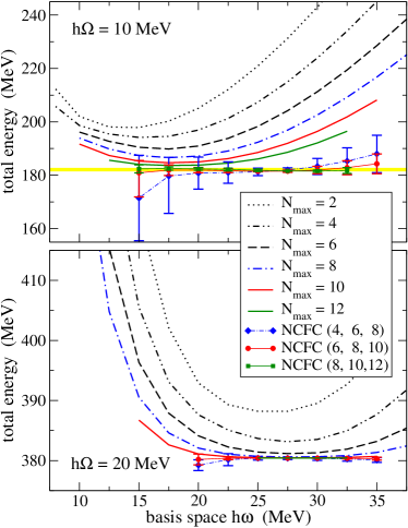
Figure 2: (color online) Ground state energy for 10 neutrons in a HO well of 10 MeV (top) and 20 MeV (bottom) for a series of finite basis space calculations with JISP16. Note that our results in the 20 MeV well converge much more rapidly than in the 10 MeV well. The symbols represent extrapolated results as discussed in the text and the error bars signify our uncertainty estimate at that basis space $\hbar\omega$; the yellow band represents our final result including numerical error estimates.

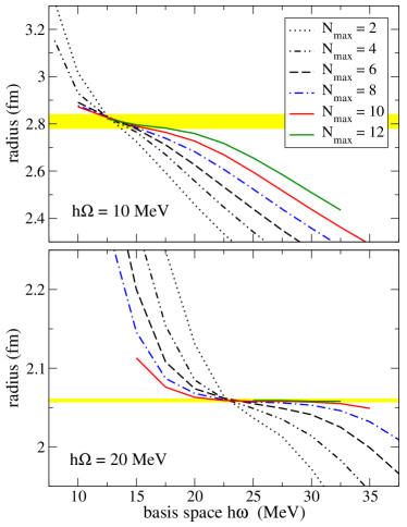
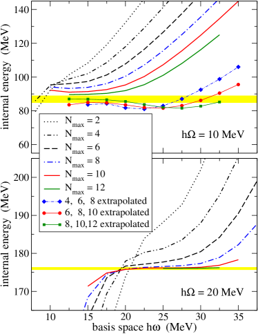
Figure 3: (color online) The rms radius (left) and internal energy (right) for 10 neutrons in a HO well of 10 MeV (top) and 20 MeV (bottom) for a series of finite basis space calculations with JISP16. Note that our results in the 20 MeV well converge much more rapidly than in the 10 MeV well. The yellow band represents our best estimate (including an error estimate) for the infinite basis space result.

For a reasonable range of basis space parameters $\hbar\omega$, this assumption appears to be valid, as is evident from Fig. 2. In this figure we show the ground state energies for 10 neutrons in a 10 MeV and 20 MeV HO well for a series of finite bases, as well as the extrapolations with their uncertainties indicated by error bars. The error bars on the extrapolations using calculations up to $N_{\hbox{\scriptsize max}}=10$ are all smaller than the corresponding error bars from calculations up to $N_{\hbox{\scriptsize max}}=8$; and the error bars on the extrapolations using calculations up to $N_{\hbox{\scriptsize max}}=12$ are all smaller than the corresponding error bars from $N_{\hbox{\scriptsize max}}=10$. Furthermore, we see that the dependence on the basis space $\hbar\omega$ decreases with increasing $N_{\hbox{\scriptsize max}}$, and that the extrapolated results for a given $N_{\hbox{\scriptsize max}}$ agree within each other’s error bars. Our total error estimate is based on a 5 MeV region in $\hbar\omega$ which has the smallest error bars and minimal $\hbar\omega$ dependence.

In order to perform this extrapolation to the infinite basis space, we need finite basis space calculations up to $N_{\hbox{\scriptsize max}}=8$ or higher. Above 22 neutrons, our calculations are limited to $N_{\hbox{\scriptsize max}}=4$, so we only have variational upper bounds for the total energy of these larger neutron drops. For the 10 MeV HO well, our results are not yet converged at this basis space, but for the 20 MeV HO well, these upper bounds are likely to be within a few percent of the converged results.

The internal energies and the rms radii do not converge monotonically with $N_{\hbox{\scriptsize max}}$, in contrast to the total energy. Currently, we do not have a reliable method to perform the extrapolation to the infinite basis space for these observables. The rms radius seems to converge from above for small basis space parameters $\hbar\omega$, but from below for large basis space parameters, see the left panels of Fig. 3. Hence there is a ’sweet spot’ in the basis space parameter $\hbar\omega$ for which the radius and equivalently, the external energy $\langle U_{\hbox{\scriptsize ext}}\rangle$, is approximately independent of $N_{\hbox{\scriptsize max}}$. We use our results in this region as an estimate of the infinite basis space result, with error bars based on the residual $N_{\hbox{\scriptsize max}}$ and $\hbar\omega$ dependence in a window around the ’sweet spot’, as indicated by the yellow band in the left panels of Fig. 3.

The internal energy appears to converge from above, at least for $\hbar\omega$ values in the region that is optimal for the total and external energies. However, we have not been able to find a robust convergence pattern; e.g. an exponential extrapolation does not work very well, as can be seen in the top right panel of Fig. 3. The most reliable estimate for the internal energy in the infinite basis space appears to be the difference between the (extrapolated) total energy and the external energy based on the convergence at the ’sweet spot’ explained above, $E_{\hbox{\scriptsize int}}=\langle H\rangle-\langle U_{\hbox{\scriptsize ext}}\rangle$. This is depicted by the yellow band in the right panels of Fig. 3.

In order to make a meaningful estimate of the converged (NCFC) results for the rms radius and the external and internal energies, we need to perform a set of calculations for a range of basis space parameters $\hbar\omega$ at least up to $N_{\hbox{\scriptsize max}}=10$. We therefore give these results only up to 14 neutrons.

V Results for neutron drops

V.1 Total energy

		5 MeV HO well		10 MeV HO well		20 MeV HO well		WS well
$N$	$J^{\pi}$	AV8′+UIX	JISP16	AV8′+UIX	JISP16	AV8′+UIX	JISP16	AV8′+UIX
3	$\frac{1}{2}^{-}$	$22.89$	$22.73(1)$	$46.69(1)$	$46.512$	$97.1(1)$	$98.094$
3	$\frac{3}{2}^{-}$	$22.61$	$22.40(1)$	$45.48(0)$	$44.833$	$91.7(1)$	$90.915$
4	$0^{+}$	$29.99$	$29.69(1)$	$62.04(1)$	$60.842$	$131.1(1)$	$126.31$
5	$\frac{1}{2}^{-}$	$41.22(1)$	$40.65(15)$	$84.02(2)$	$82.86(2)$	$175.2(1)$	$173.00$
5	$\frac{3}{2}^{-}$	$41.02$	$40.4(2)$	$82.97(1)$	$80.68(2)$	$169.5(1)$	$162.71$
6	$0^{+}$	$48.52(1)$	$47.6(2)$	$98.95(2)$	$95.74(3)$	$205.8(2)$	$193.64$	$-80.6\hphantom{(1)}$
7	$\frac{1}{2}^{-}$	$59.17(1)$	$57.9(2)$	$118.9(0)$	$115.67(5)$	$246.4(2)$	$237.11$	$-90.9(1)$
7	$\frac{3}{2}^{-}$	$59.73(1)$	$58.5(2)$	$121.1(0)$	$118.9(1)$	$254.7(2)$	$249.85$	$-88.6(1)$
8	$0^{+}$	$67.01(1)$	$65.4(3)$	$135.8(0)$	$132.5(1)$	$287.4(2)$	$278.32(1)$	$-103.9(1)$
9	$\frac{1}{2}^{+}$	$80.92(4)$	$78.9(1.5)$	$163.7(1)$	$159.6(4)$	$349.8(2)$	$334.32(1)$	$-107.8(1)$
9	$\frac{3}{2}^{+}$		$80.0(1.5)$		$162.8(6)$	$354.5(2)$	$344.42(1)$
9	$\frac{5}{2}^{+}$	$81.20(3)$	$79.3(1.5)$	$163.2(1)$	$159.4(4)$	$343.9(2)$	$331.15(1)$	$-106.6(1)$
10	$0^{+}$	$92.14(8)$	$90.(1.5)$	$188.1(6)$	$182.1(5)$	$400.5(2)$	$380.41(1)$	$-113.4(1)$
11	$\frac{1}{2}^{+}$	$105.9(1)$		$216.1(3)$	$208.4(1.0)$		$434.38(5)$	$-115.9(2)$
11	$\frac{3}{2}^{+}$				$208.0(1.0)$		$430.10(4)$
11	$\frac{5}{2}^{+}$	$106.3(1)$		$217.0(3)$	$207.9(1.0)$		$430.41(4)$	$-116.9(2)$
12	$0^{+}$	$118.1(1)$	$116.(6)$	$242.(1)$	$230.0(1.0)$	$509.1(4)$	$477.05(5)$	$-123.6(3)$
13	$\frac{1}{2}^{+}$	$130.8(1)$		$268.0(1.0)$	$255.8(1.0)$		$529.07(6)$	$-125.0(3)$
13	$\frac{3}{2}^{+}$				$256.3(1.0)$		$528.74(6)$
13	$\frac{5}{2}^{+}$	$131.5(1)$		$267.6(6)$	$255.7(1.0)$		$524.77(6)$	$-125.9(3)$
14	$0^{+}$	$142.2(2)$	$140.(10)$	$291.9(2)$	$277.5(1.4)$		$569.3(1)$	$-131.6(7)$
15	$\frac{1}{2}^{+}$	$160.1(1)$		$316.3(2)$	$303.(5)$		$619.4(6)$
15	$\frac{3}{2}^{+}$	$159.1(2)$		$320.2(2)$
15	$\frac{5}{2}^{+}$	$160.0(1)$		$317.0(2)$				$-139.3(3)$
16	$0^{+}$	$171.6(1)$		$341.5(2)$	$326.(6)$	$730.3(3)$	$667.7(6)$	$-142.4(7)$
17	$\frac{1}{2}^{+}$	$185.5(2)$		$368.8(3)$			$725.1(8)$
17	$\frac{3}{2}^{+}$	$183.9(2)$		$366.5(3)$	$352.(5)$			$-148.8(2)$
17	$\frac{5}{2}^{+}$	$184.9(2)$		$371.1(2)$
18	$0^{+}$	$195.6(2)$		$392.6(3)$	$377.(7)$		$781.(1)$	$-155.1(4)$
19	$\frac{1}{2}^{+}$	$209.4(2)$		$420.1(2)$	$407.(7)$	$919.0(3)$	$850.(2)$
19	$\frac{3}{2}^{+}$	$208.4(2)$		$417.9(3)$	$403.(7)$	$914.9(4)$	$838.(1)$	$-159.6(3)$
19	$\frac{5}{2}^{+}$	$210.0(3)$		$422.1(2)$	$408.(8)$	$926.7(4)$	$855.(2)$
20	$0^{+}$	$219.9(3)$		$441.7(4)$	$430.(10)$	$976.0(4)$	$894.(2)$	$-165.0(1)$
21	$\frac{7}{2}^{-}$			$476.8(4)$	$465.(25)$		$956.(4)$
22	$0^{+}$	$254.(1)$		$510.5(5)$	$495.(25)$	$1123.3(7)$	$1018.(5)$
24	$0^{+}$	$289.1(7)$		$578.9(5)$	$<596.$	$1268.(1)$	$\leq 1144.$
26	$0^{+}$	$324.0(8)$		$645.0(6)$	$<660.$		$\leq 1266.$
28	$0^{+}$	$355.(1)$		$707.6(7)$	$<723.$	$1551.(1)$	$\leq 1379.$
30	$0^{+}$	$390.0(8)$		$776.0(9)$	$<786.$		$\leq 1499.$
32	$0^{+}$	$422.(1)$		$843.5(9)$	$<847.$		$\leq 1614.$
34	$0^{+}$	$453.(1)$		$909.9(9)$	$<914.$		$\leq 1750.$
36	$0^{+}$	$486.(1)$		$982.7(8)$	$<986.$		$\leq 1895.$
38	$0^{+}$	$514.(1)$		$1046.4(8)$	$<1057.$		$\leq 2037.$
40	$0^{+}$	$546.(1)$		$1114.3(9)$	$<1128.$		$\leq 2177.$
42	$0^{+}$	$591.(1)$		$1197.1(8)$	$<1206.$		$\leq 2320.$
44	$0^{+}$			$1278.(1)$			$\leq 2473.$

Table 2: Total energy with AV8^′+UIX and JISP16 for several different confining wells. Error bars for the AV8^′+UIX results are statistical only; in addition we expect systematic errors of a few percent, as discussed in Sec. III.4. Error bars for the JISP16 results are total error estimates. (Errors that are not shown are less than 1 in the last digit.)

In Table 2 we present the principal results of this study: the total energies for neutron drops confined in 5 MeV, 10 MeV, and 20 MeV HO wells with the AV8^′+UIX and JISP16 potentials. These HO wells are convenient for ab-initio calculations because one can probe very low to very high densities with a simple asymptotic form of the wave function and an arbitrary number of neutrons can be bound in the well. In order to provide a very different probe of density functionals in the extreme isospin limit, we also include select results in a WS well with the AV8^′+UIX potential.

We show the lowest 0⁺ energy for even $N$ and lowest values for several $J^{\pi}$ for odd $N$. We present results only for natural parity states. The AV8^′+UIX values up to $N$=14 were computed by GFMC while the larger drops were computed using AFDMC, with the exception of the 20 MeV HO well results. There are no results from GFMC available for the 20 MeV HO well, due to the strong fermion sign problem with that external field strength; those results were all obtained using AFDMC.

The JISP16 values were all computed by NCFC. There are no results from NCFC available in the 5 MeV trap above 14 neutrons due to poor convergence with available computer resources. Above 22 neutrons we only provide strict upper bounds; for the 20 MeV HO well we expect the converged energies to be within a few percent of these upper bounds.

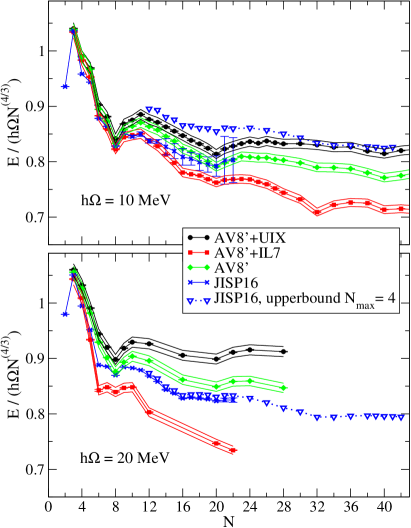
Figure 4: (color online) Energy of the lowest neutron drop states confined in a HO well with $\hbar\Omega=10$ MeV (top) and $\hbar\Omega=20$ MeV (bottom) as a function of the number of neutrons. Results for AV8^′ (plus TNI) where obtained using AFDMC, with MC statistical error bars as well as a band indicating the 1% systematic uncertainty discussed in Sec. III.4; results for JISP16 are obtained from NCFC with error bars reflecting the total numerical uncertainty, and strict upper bounds obtained with NCSM in finite basis spaces. Note the pronounced dips at the expected HO magic numbers $N=2$, $8$, and $20$.

Figure 4 shows the energies of $N$ neutrons in two different HO wells, scaled by $\hbar\Omega\,N^{(4/3)}$; for odd $N$ only the lowest energy found is shown. The scaling by $\hbar\Omega\,N^{(4/3)}$ is motivated by the expected results in local density approximation. The factor $N^{4/3}$ comes from the traditional scaling with $N$ times the increase in potential energy arising from the increase in radius of the system with particle number proportional to $N^{1/3}$. In addition to the AV8^′+UIX and JISP16 values presented in Table 2, we also show results for AV8^′ without any TNI and AV8^′+IL7. All interactions show a very pronounced peak for three neutrons, and dips at the expected HO magic numbers, $N=2$, $8$, $20$, and $40$. The dips at the HO magic numbers are expected due to the HO nature of the confining well.

With an equation of state of the form $E=\xi\frac{\hbar^{2}}{2m}k_{F}^{2}$ with $k_{F}=[3\pi^{2}\rho]^{1/3}$, the energy is given by the Thomas–Fermi expression: $E_{TF}=\xi^{1/2}\hbar\Omega\,(3N)^{(4/3)}/4$. For free fermions ($\xi=1$) the Thomas–Fermi results would be a horizontal line at $3^{4/3}/4\approx 1.081$, for a unitary Fermi gas with $\xi=0.4$ the Thomas–Fermi results would be a horizontal line at 0.684. The calculated results are all below the free Fermi gas (even for the case of three neutrons) since the interaction is attractive. All our results are above the unitary Fermi gas because there are significant finite-range corrections for neutron matter. In addition repulsive gradient terms in the density functional are required to reproduce the ab-initio results Gandolfi et al. (2011). A detailed investigation of these effects is being pursued.

From Fig. 4 it is evident that adding UIX to AV8^′ increases the energies of neutron drops, whereas IL7 decreases the energies. These results were expected; the two-pion part of UIX is attractive in the isospin $T=1/2$ triples that appear in nuclei. However neutron drops contain only $T=3/2$ triples for which the two-pion part is very small Pudliner et al. (1996); Gandolfi et al. (2012); this leaves only the repulsive central part of UIX. On the other hand, IL7 contains the three-pion term that is strongly attractive in $T=3/2$ triplets Pieper et al. (2001).

The energies with the nonlocal 2-body interaction JISP16 are generally below the AV8^′ results, but above the AV8^′+IL7 ground state energies. In fact, in the 10 MeV HO trap, the JISP16 results are nearly identical to those with AV8^′+IL7 up to about 12 neutrons; as the number of neutrons increases, the results with JISP16 deviate more and more from the AV8^′+IL7 results. In the 20 MeV HO trap, for which we have more accurate results with JISP16, the results with JISP16 and with AV8^′ without TNI are quite similar, even in the $sd$-shell and beyond. The trend of the upper bounds obtained with JISP16 follows the trend of the AV8^′ ground state energies through the $sd$-shell and into the $pf$-shell, both in the 10 MeV and in the 20 MeV trap.

As discussed in Sec. II.1 and in Sec. VI below, recent studies of the neutron star mass-radius relationship Steiner and Gandolfi (2012); Gandolfi et al. (2012) suggest that, at least at higher densities, the AV8^′ + UIX interactions gives a reasonable neutron matter equation of state. The requirement of a two-solar mass neutron star implies a repulsive three-neutron interaction at moderate and high densities.

On the other hand, AV8^′+IL7 gives a much better description of the ground state energies, spectra, and other observables for light nuclei (up to $A=12$) than either AV8^′ or AV8^′+UIX. This may be why the results with AV8^′+IL7 and with JISP16 (which also gives a good description of light nuclei) are quite similar below 12 neutrons. However, none of these interactions have been fit to any data beyond the $p$-shell, and it is unclear which of these interactions is more realistic for the neutron drops in the $N=8$ to $N=40$ range. At larger densities AV8^′+IL7 is too attractive as discussed below.

In the 10 MeV well, the dips in the energies at $N=16$ and $N=32$ suggest subshell closure with AV8^′+IL7, but not with AV8^′+UIX, while the results for AV8^′ show a hint of subshell closure at $N=32$. The IL7 TNI does provide a larger spin-orbit splitting than the UIX three-nucleon interaction. Similarly, the energies with JISP16 suggest subshell closure at $N=16$ and $N=32$ in the 20 MeV well. The JISP16 results in the 10 MeV well are not quite accurate enough to draw firm conclusion regarding subshell closure; and we have insufficient results for AV8^′ in the 20 MeV well.

Somewhat surprisingly, there is no indication of subshell closure at $N=28$. In other words, these results seem to suggest closure of the combined $f_{\frac{7}{2}}$ and $p_{\frac{3}{2}}$ subshell at $N=32$, rather than closure of just the $f_{\frac{7}{2}}$ at $N=28$. Note that the closure of the combined $d_{\frac{5}{2}}$ and $s_{\frac{1}{2}}$ subshell at $N=16$ corresponds to the recently discovered subshell closure at ²⁴O Mueller et al. (1990).

V.2 Energy differences

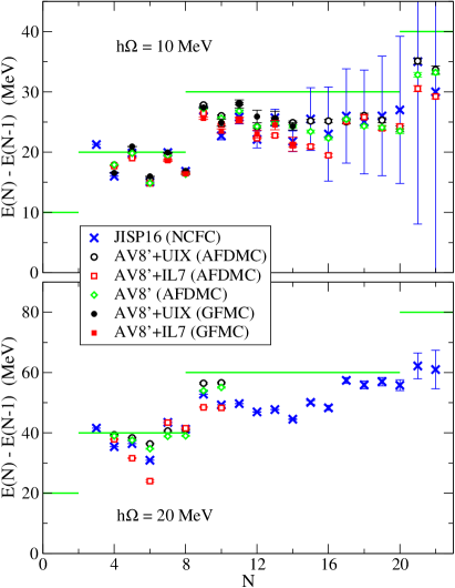
Figure 5: (color online) Single energy differences in a 10 MeV (top) and 20 MeV (bottom) HO well. Results of different Hamiltonians are compared. AFDMC and GFMC error bars are statistical only; NCFC error bars reflect the total numerical uncertainty. Horizontal line segments indicate energy differences expected from pure HO energies.

In Fig. 5 we show the difference in total energy between neutron drops with $N$ and with $N-1$ neutrons. We clearly see the effect of the HO shells: jumps at 2, 8, and 20 neutrons, at which the next neutron has to go to the next HO shell. Without interactions between the neutrons, we would still have this shell structure, but within each shell, all single energy differences would be equal, as indicated by the solid reference lines in Fig. 5. That is, the gross feature of shell structure arises from the confining well and is evident in the plot of the single differences as a jump in the calculated energy differences as one goes from one shell to the next.

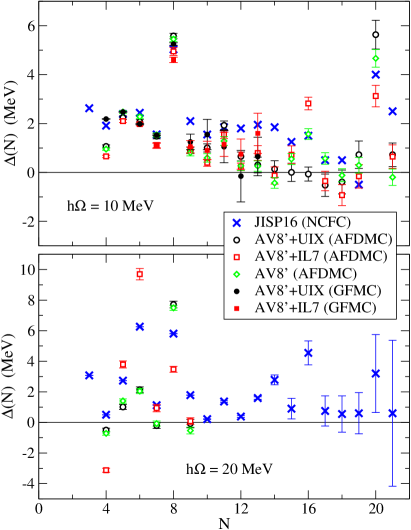
Figure 6: (color online) Double energy differences $\Delta(N)=(-1)^{N+1}[E(N)-\frac{1}{2}\left(E(N-1)+E(N+1)\right)]$ in a 10 MeV (top) and 20 MeV (bottom) HO well. Results of different Hamiltonians are compared. AFDMC and GFMC error bars are statistical only; the NCFC error bars are omitted for the 10 MeV HO well, because they would cover the entire vertical range for 12 neutrons and above, though a significant part of the NCFC numerical error is systematic, and cancels between neighboring neutron drops; for completeness, we did include the total numerical uncertainty for the NCFC results in the 20 MeV HO well.

The detailed fluctuations within a shell are entirely due to the neutron interactions. The most prominent feature is the neutron pairing, in particular in the $p$-shell and also in the (beginning) of the $sd$-shell. This effect can be seen more clearly by looking at the double difference in total energy $\Delta(N)=(-1)^{N+1}[E(N)-\frac{1}{2}\left(E(N-1)+E(N+1)\right)]$, see Fig. 6. The phase $(-1)^{N+1}$ is included to make the pairing positive definite in the standard BCS theory. Without interactions, the double differences would be zero, except at the magic numbers 2, 8, and 20.

Overall, the pairing seems to decrease as $N$ increases, except for the closed (sub)shells. Note that the pairing in nuclei also decreases for larger nuclei Robledo and Bertsch (2012). On the other hand, the numerical uncertainties increase with $N$, preventing us from obtaining meaningful results for the pairing beyond 22 neutrons using the NCFC approach. AFDMC calculations of the pairing gaps will be more reliable once BCS correlations have been included in the trial state and this is being pursued. For all methods we expect that the error in neighboring neutron drops is correlated, resulting in a reduced error in calculations of energy differences and pairing.

Despite the numerical uncertainties, there are some features that are likely to be robust in Fig. 6. As expected, the peaks in the double difference $\Delta(N)$ at the magic numbers 8 and 20 stand out for all of the interactions for which we have results, in particular for the 10 MeV HO well. In addition, our results suggest subshell closure at $N=16$ for AV8^′ without TNIs, with AV8^′+IL7, and with JISP16, but not with AV8^′+UIX. This closed subshell corresponds to the recently discovered subshell closure at ²⁴O Mueller et al. (1990), in which TNIs play a crucial role.

In addition to the closure at $N=16$, we see evidence for subshell closure at $N=6$ (the $p_{\frac{3}{2}}$) in the 20 MeV HO well both with AV8^′+IL7 and with JISP16, but not in the 10 MeV HO well. We do not have sufficient data yet to examine the expected closure of the $f_{\frac{7}{2}}$ at $N=28$, which was not evident in the plots of the total energy (see Fig. 4), nor for a more detailed analysis of the closure at $N=32$ suggested in Fig. 4.

V.3 Level splittings

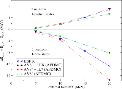
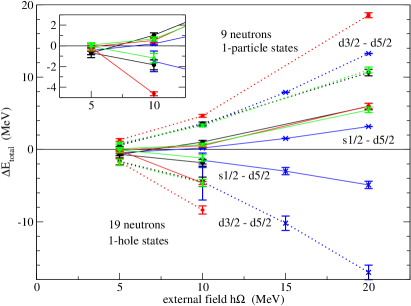
Figure 7: (color online) Spin-orbit splitting in the $p$-shell (top) and level splittings in the $sd$-shell (bottom) and as a function of external field strength. Results of different Hamiltonians are compared. Inset: blowup of the $s_{\frac{1}{2}}$ and $d_{\frac{5}{2}}$ levels for the 5 MeV and 10 MeV H.O. wells.

If we look at the single-particle and single-hole states at the beginning and end of the $p$-shell, see Fig. 7, we find that the spin-orbit splitting between the $\frac{1}{2}^{-}$ and $\frac{3}{2}^{-}$ increases with $\hbar\Omega$ for all interactions. For three neutrons, the splitting between these levels is almost the same for JISP16 and AV8^′+IL7; however, for seven neutrons the splitting is significantly enhanced with IL7. On the other hand, AV8^′ without TNI and AV8^′+UIX have almost the same splitting.

The systematic increase in level splittings with increasing $\hbar\Omega$ can be understood as follows: With increased $\hbar\Omega$, the radial shape is increasingly constrained by the HO potential and the associated gaussian falloff of the radial densities in the surface region. This increase in level splittings with $\hbar\Omega$ may then be interpreted as a consequence of the increased density gradient in the surface region.

In the $sd$-shell the splitting between the $d_{\frac{5}{2}}$ and $s_{\frac{1}{2}}$ levels (solid lines in Fig. 7) is much smaller than the splitting between these two levels and the $d_{\frac{3}{2}}$ level, in particular for AV8^′+IL7. This confirms the subshell closure at $N=16$ that was evident from the pairing, see Fig. 6. It is also in apparent agreement with the observation in known nuclei that the subshell closure at 16 neutrons (both $d_{\frac{5}{2}}$ and $s_{\frac{1}{2}}$ levels filled) is much stronger than the subshell closure at 14 neutrons (only the $d_{\frac{5}{2}}$ level filled).

Furthermore, notice that the level ordering can change as the strength of the HO well increases in the case of 9 neutrons: in the weakest well of 5 MeV (i.e. at very low density), the $s_{\frac{1}{2}}$ is slightly below the $d_{\frac{5}{2}}$ level, but as $\hbar\Omega$ increases, the $d_{\frac{5}{2}}$ becomes the lowest level. Interestingly, this happens both with JISP16 and with AV8^′+IL7, whereas with AV8^′+UIX and with AV8^′ (without TNIs) the $d_{\frac{5}{2}}$ and $s_{\frac{1}{2}}$ are basically degenerate for the 5 MeV HO well.

In the $pf$-shell we find qualitatively similar results with JISP16: a large spin-orbit splitting between the $f_{\frac{7}{2}}$ and $f_{\frac{5}{2}}$ levels and between the $p_{\frac{3}{2}}$ and $p_{\frac{1}{2}}$ levels, a smaller splitting between the $p_{\frac{1}{2}}$ and $f_{\frac{5}{2}}$ levels, and an even smaller splitting between the $f_{\frac{7}{2}}$ and $p_{\frac{3}{2}}$ levels. All of these level splittings increase significantly with the strength of the HO well: at $\hbar\Omega=5$ MeV, the splittings are almost negligible, less than an MeV, and within the numerical uncertainty. On the other hand, at $\hbar\Omega=20$ MeV (the largest value that we have considered) the spin-orbit splittings are of the order of ten(s) of MeV.

V.4 Internal energies and radii

		5 MeV HO well				10 MeV HO well				20 MeV HO well		WS well
$N$	$J^{\pi}$	AV8′+UIX		JISP16		AV8′+UIX		JISP16		JISP16		AV8′+UIX
3	$\frac{1}{2}^{-}$	$11.5$	$3.56$	$11.2$	$3.58$	$22.3$	$2.60$	$22.02$	$2.60$	$44.31$	$1.928(1)$
3	$\frac{3}{2}^{-}$	$11.3$	$3.52$	$11.2$	$3.51$	$22.3$	$2.53$	$22.26$	$2.50$	$43.80$	$1.805(1)$
4	$0^{+}$	$14.8$	$3.55$	$14.4$	$3.56$	$29.1$	$2.61$	$29.10$	$2.57$	$58.92$	$1.869(1)$
5	$\frac{1}{2}^{-}$	$20.6$	$3.70$	$20.1(2)$	$3.70(2)$	$40.1$	$2.70$	$39.8$	$2.67$	$79.5$	$1.969(2)$
5	$\frac{3}{2}^{-}$	$20.6$	$3.68$	$20.3(2)$	$3.65(2)$	$40.0$	$2.70$	$40.5$	$2.58$	$78.5$	$1.869(2)$
6	$0^{+}$	$24.2$	$3.67$	$23.8(4)$	$3.63(3)$	$47.3$	$2.67$	$47.8$	$2.58$	$92.8$	$1.867(1)$	$46.9$	$2.70$
7	$\frac{1}{2}^{-}$	$29.7$	$3.74$	$29.7(5)$	$3.66(3)$	$56.8$	$2.71$	$57.3(2)$	$2.63$	$111.3(1)$	$1.930(2)$	$55.6$	$2.75$
7	$\frac{3}{2}^{-}$	$29.9$	$3.76$	$29.7(5)$	$3.70(3)$	$57.2$	$2.75$	$56.9(2)$	$2.71$	$113.2(1)$	$2.012(2)$	$55.2$	$2.81$
8	$0^{+}$	$35.0$	$3.64$	$33.2(6)$	$3.65(3)$	$64.4$	$2.72$	$63.5(2)$	$2.68(1)$	$126.2(1)$	$1.986(2)$	$63.2$	$2.75$
9	$\frac{1}{2}^{+}$	$41.9$	$3.79$	$40.(2)$	$3.77(5)$	$77.9$	$2.81$	$76.5(1.)$	$2.77(2)$	$152.7(2)$	$2.045(2)$	$70.5$	$3.03$
9	$\frac{3}{2}^{+}$			$41.(2)$	$3.82(5)$			$77.1(1.)$	$2.81(3)$	$155.2(2)$	$2.088(2)$
9	$\frac{5}{2}^{+}$	$42.2$	$3.79$	$41.(2)$	$3.78(5)$	$78.3$	$2.80$	$77.4(1.)$	$2.75(2)$	$153.2(2)$	$2.024(2)$	$73.6$	$2.93$
10	$0^{+}$	$46.7$	$3.88$	$45.(2)$	$3.85(10)$	$88.$	$2.89$	$87.0(1.)$	$2.81(2)$	$176.0(3)$	$2.059(2)$	$78.$	$3.11$
11	$\frac{1}{2}^{+}$	$53.7$	$3.97$			$99.$	$2.97$	$100.(2.)$	$2.86(3)$	$201.7(8)$	$2.095(4)$	$89.$	$3.21$
11	$\frac{3}{2}^{+}$							$101.(2.)$	$2.84(3)$	$202.1(5)$	$2.074(3)$
11	$\frac{5}{2}^{+}$	$53.2$	$4.00$			$102.$	$2.95$	$100.(2.)$	$2.85(3)$	$202.1(5)$	$2.075(3)$	$87.$	$3.23$
12	$0^{+}$	$59.4$	$4.03$			$110.$	$3.02$	$110.(2)$	$2.88(3)$	$224.0(5)$	$2.090(3)$	$97.$	$3.20$
13	$\frac{1}{2}^{+}$	$65.5$	$4.08$			$121.$	$3.06$	$123.(2)$	$2.91(3)$	$248.5(6)$	$2.116(3)$	$106.$	$3.29$
13	$\frac{3}{2}^{+}$							$123.(2)$	$2.91(3)$	$249.5(6)$	$2.111(3)$
13	$\frac{5}{2}^{+}$	$65.9$	$4.09$			$120.$	$3.06$	$124.(2)$	$2.90(3)$	$249.9(6)$	$2.094(3)$	$103.$	$3.37$
14	$0^{+}$	$71.1$	$4.10$			$132.$	$3.08$	$134.(3)$	$2.92(4)$	$271.8(7)$	$2.099(3)$	$115.$	$3.31$

Table 3: Internal energies (in MeV) and rms radii (in fm) of neutron drops with various external potentials and a selected set of Hamiltonians. The results are plotted in Figs. 8 and 9. The particular many-body method used to produce these results depends on the external field, the number of neutrons and the Hamiltonian as described in the text.

In Table 3 we list our results for the internal energy $E_{\hbox{\scriptsize int}}=\langle H\rangle-\langle U_{\hbox{\scriptsize ext}}\rangle$, as well as for the rms radii for systems up to 14 neutrons in a HO well with JISP16 and with AV8^′+UIX, as well as in a WS well with AV8^′+UIX. Note that for neutron drops in a HO well the radius is directly related to the external energy, $\langle U_{\hbox{\scriptsize ext}}\rangle=\frac{1}{2}m\omega^{2}\langle r^{2}\rangle$ for a HO external field. Overall, the internal energy is typically slightly less than half of the total energy (see Table 2 for comparison), and $\langle U_{\hbox{\scriptsize ext}}\rangle$ is slightly more than half the total energy. This is to be expected, since the total energy scales approximately as $\hbar\Omega\,N^{(4/3)}\propto\rho^{2/3}$, and for all cases where the equation of state is proportional to $\rho^{2/3}$, the virial theorem will give equal internal energies and one-body potential energies, each one-half of the total energy.

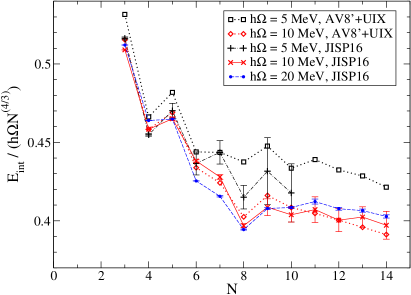
Figure 8: (color online) Internal energy for up to 14 neutrons in a HO trap with AV8^′+UIX and with JISP16. For details see Table 3.

In Fig. 8 we show the internal energy $E_{\hbox{\scriptsize int}}$, scaled by $\hbar\Omega\,N^{(4/3)}$, of the lowest $J=0$ and $J=\frac{1}{2}$ states for up to 14 neutrons in a HO well. In the 10 MeV trap the JISP16 and the AV8^′+UIX results are rather close to each other, significantly closer than the total energies shown in Fig. 4. Apparently, the larger differences observed in Fig. 4 arise primarily from differences in their $\langle U_{\hbox{\scriptsize ext}}\rangle$ energy shifts. Indeed, the corresponding rms radii, and thus $\langle U_{\hbox{\scriptsize ext}}\rangle$, start to deviate from each other above $N=10$, see Fig. 9.

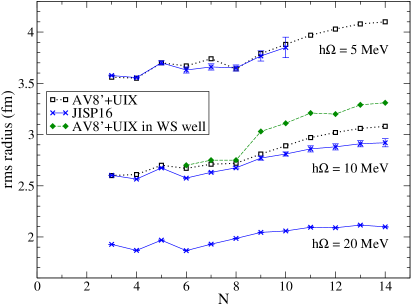
Figure 9: (color online) Radii for the lowest $J$ states up to 14 neutrons in a HO trap with AV8^′+UIX and with JISP16. For details see Table 3.

The two interactions also give quite similar internal energy results in the 5 MeV trap as seen in Fig. 8, given the rather large error bars of the NCFC results, and the corresponding radii are almost identical, at least up to 10 neutrons.

Table 3 shows that both the internal energies and the rms radii in the WS well are of the same order as those in the 10 MeV HO trap, even though the total energies are very different. In fact, the rms radii are nearly identical for the three $p$-shell neutron drops ($N=6$, $7$, and $8$), but in the $sd$-shell there are significant differences between the HO and the WS radii.

We note that the internal energy Fig. 8 displays a similar odd-even effect due to pairing as we observed in the total energy in Fig. 4. The radii of the $J=0$ and $J=\frac{1}{2}$ states also show an odd-even effect, but only in the $p$-shell, for three to seven neutrons; there is no a significant odd-even effect for these states above $N=8$ in Fig. 9. Also note that the radii of states with different $J$ in odd neutron systems are slightly different, in particular in the $p$-shell, and more so with JISP16 than with AV8^′ + UIX, as can be seen in Table 3.

V.5 Densities

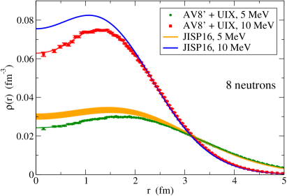
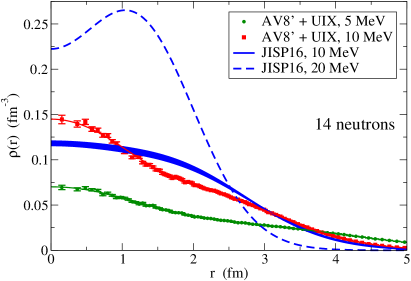
Figure 10: (color online) Radial density distributions for 8 (top) and 14 (bottom) neutrons in different HO traps with JISP16 and with AV8^′+UIX.

We present a sample set of radial density distributions computed with JISP16 and with the AV8^′+UIX Hamiltonian in Fig. 10. The band thickness of the JISP16 results, obtained with NCFC, is our best estimate of the total numerical uncertainty in these densities; the AV8^′+UIX results were calculated with GFMC, and the error bars correspond to the statistical errors in the GFMC approach. Given the HO nature of the trap, all density distributions fall like gaussians at distances sufficiently far from the origin.

The various densities for 8 neutrons (top panel of Fig. 10, closed $p$-shell) are quite similar for the two different interactions. The only difference is that the central densities, below 1 fm, are about 10% to 20% higher with JISP16 than with AV8^′+UIX, but the shape is essentially the same, and above 2 to 3 fm the densities are practically on top of each other. This could be expected from the similar rms radii for these cases shown in Table 3. As the HO trap strength increases, the density distribution gets compressed, the rms radius decreases, and the central density increases, as one would expect. The radial shape, a slight dip at $r=0$, is typical for the closed $p$-shell, and is qualitatively the same for weak and strong HO traps.

However, the shape of the density profile for 14 neutrons is somewhat different for the two interactions; furthermore, the shape seems to depend on the strength of the HO trap, at least for JISP16. With JISP16 in the 20 MeV trap (dashed curve in the bottom panel of Fig. 10), the density has a clear dip at the center, and peaks at a distance of about 1 fm from the center. In fact, the shape of this density is rather similar to that of 8 neutrons in a HO trap. On the other hand, in the 10 MeV trap there is no evidence for such a dip; rather, within the estimated numerical accuracy, the density seems to fall off monotonically from a central value of about 0.11 to 0.12 fm^-3 with JISP16. On the other hand, the densities obtained with the AV8^′+UIX Hamiltonian for 14 neutrons seem to be slightly enhanced in the central region: in the 10 MeV trap the central density with with the AV8^′+UIX is about 20% higher than with JISP16.

This difference between the density profiles of 14 neutrons in a HO trap with JISP16 and AV8^′+UIX could well be related to the presence (JISP16) and absence (AV8^′+UIX) of sub-shell closure for 16 neutrons; and both are likely to be related to differences in spin-orbit splittings. It would be interesting to compare these densities with those obtained with other realistic potentials, and in particular to investigate the effect of different 3-body forces on the density profiles as well as on the spin-orbit splittings and sub-shell closures.

VI Neutron matter

The equation of state of neutron matter is important to properly fix the bulk term of Skyrme-type EDFs. We report the AFDMC results for the energy per neutron as a function of the density in Table 4 and display them in Fig. 11. For the AFDMC Quantum Monte Carlo calculations, the results are for a system of 66 neutrons with periodic boundary conditions. The calculation is very similar to those of the neutron drops, except the single-particle orbitals in the trial wave function are replaced by plane waves that respect the periodic boundary condition, as described in Sec. III.3. More details can be found in Refs. Gandolfi et al. (2009a); Sarsa et al. (2003). The energy corrections due to finite-size effects arising from such a simulation are expected to be extremely small compared to the bulk energies considered here.

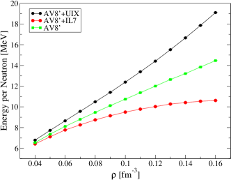
Figure 11: (color online) Equation of state of neutron matter as a function of the density for different Hamiltonians.

$\rho$ [fm-3]	AV8′	AV8′+UIX	AV8′+IL7
0.04	6.55(1)	6.79(1)	6.42(1)
0.05	7.36(1)	7.73(1)	7.11(1)
0.06	8.11(1)	8.65(1)	7.77(1)
0.07	8.80(1)	9.57(1)	8.26(1)
0.08	9.47(1)	10.49(1)	8.75(2)
0.09	10.12(1)	11.40(1)	9.14(2)
0.10	10.75(1)	12.39(1)	9.50(2)
0.11	11.37(1)	13.39(1)	9.78(2)
0.12	12.00(1)	14.42(1)	10.03(2)
0.13	12.64(1)	15.52(1)	10.27(2)
0.14	13.21(1)	16.66(1)	10.41(2)
0.15	13.84(2)	17.87(2)	10.54(3)
0.16	14.47(2)	19.10(2)	10.62(3)

Table 4: Equation of state of neutron matter as a function of the density for various Hamiltonians.

The effect of TNI is important in the equation of state of neutron matter beyond half nuclear matter saturation density ($\rho=0.08~{}{\rm fm}^{-3}$), as is clear in Fig. 11. The two different TNIs added to AV8^′ have opposite effects: UIX is repulsive, while IL7 is attractive. This is in agreement with the trend in neutron drops shown in Fig. 4. Our earlier discussion of the effects of the different terms in UIX and IL7 apply equally to the differences observed here. Furthermore, in moderately large neutron drops ($N>12$) we have seen that the trend with JISP16 is similar to the trend with AV8^′ without TNI. We therefore expect that the equation of state with JISP16 will be similar to that of AV8^′ without TNIs.

The equation of state of pure neutron matter with the AV8^′ NN interaction alone is rather soft at high densities. It is only marginally compatible with the recently-observed two-solar mass neutron star Demorest et al. (2010); Gandolfi et al. (2012); Akmal et al. (1998); Steiner and Gandolfi (2012). The relevant three-neutron force must be, in aggregate, repulsive at high densities Akmal et al. (1998). While the three-pion terms in IL7 (and in $\chi$PT forces) are certainly present, they are far too attractive in the IL7 model alone. It is possible to adjust the short- and long-range three neutron forces to be repulsive by varying the contributions of these magnitudes, as obtained in the recent studies of three-neutron interactions and the neutron star mass-radius relations Gandolfi et al. (2012).

VII Conclusions

We have computed the properties of neutron drops confined by external harmonic oscillator (HO) and Woods Saxon (WS) traps using a variety of realistic nucleon-nucleon and nucleon-nucleon plus three-nucleon interactions (TNIs). The combination of results with HO and WS wells should prove useful in separating bulk and gradient (surface) effects, and testing the general form of the density functional. The pairing and spin orbit splittings may also have very different behavior.

We have employed currently available state-of-the art many-body methods to obtain these results and we have quantified the uncertainties in the results. We observe characteristic features such as pairing and subshell closures in qualitative agreement with expectations. Differences in results for the same systems are attributable in large part to differences in the interactions. We present and interpret significant sensitivity of some obervables to the TNI. The radii of the neutron drops appear to be rather robust - that is approximately independent among the interactions we employ.

The results we obtain for the neutron equation of state as a function of density follow trends seen in the neutron drop results as a function of the external HO trap. This is significant since the neutron drops have quantified uncertainties on their total and internal energies as well as their rms radii, while it is more difficult to quantify the uncertainty in the calculated neutron matter equation of state.

We anticipate that results for these extreme and idealized systems may serve as guides to experiments on very neutron-rich nuclei. We also hope these results will inform developments of improved energy-density functionals Gandolfi et al. (2011); Kortelainen et al. (2012).