Sequences with Minimal Time-Frequency Uncertainty

Abstract

A central problem in signal processing and communications is to design signals that are compact both in time and frequency. Heisenberg’s uncertainty principle states that a given function cannot be arbitrarily compact both in time and frequency, defining an “uncertainty” lower bound. Taking the variance as a measure of localization in time and frequency, Gaussian functions reach this bound for continuous-time signals. For sequences, however, this is not true; it is known that Heisenberg’s bound is generally unachievable. For a chosen frequency variance, we formulate the search for “maximally compact sequences” as an exactly and efficiently solved convex optimization problem, thus providing a sharp uncertainty principle for sequences. Interestingly, the optimization formulation also reveals that maximally compact sequences are derived from Mathieu’s harmonic cosine function of order zero. We further provide rational asymptotic expansions of this sharp uncertainty bound. We use the derived bounds as a benchmark to compare the compactness of well-known window functions with that of the optimal Mathieu’s functions.

1 Introduction

Suppose you are asked to design filters that are sharp in the frequency domain and at the same time compact in the time domain. The same problem is posed in designing sharp probing basis functions with compact frequency characteristics. In order to formulate these problems mathematically, we need to have a correct and universal definition of compactness and clarify what we mean by saying a signal is spread in time or frequency.

These notions are well defined and established for continuous-time signals [13, 34] and their properties are studied thoroughly in the literature. For such signals, we can define the time and frequency characteristics of a signal as in Table 1. Note the connection of these definitions with the mean and variance of a probability distribution function $|x(t)|^{2}/\left\|x\right\|^{2}$. The value of $\Delta_{t}^{2}$ is considered as the spread of the signal in the time domain while $\Delta_{{\omega}_{c}}^{2}$ represents its spread in the frequency domain. We say that a signal is compact in time (or frequency) if it has a small time (or frequency) spread.

domain	center	spread
time	$\mu_{t}=\frac{1}{\left\|x\right\|^{2}}\int_{t\in\mathbb{R}}t|x(t)|^{2}dt$	$\Delta_{t}^{2}=\frac{1}{\left\|x\right\|^{2}}\int_{t\in\mathbb{R}}(t-\mu_{t})^{2}|x(t)|^{2}dt$
frequency	$\mu_{{\omega}_{c}}=\frac{1}{2\pi\left\|x\right\|^{2}}\int_{{\omega}\in\mathbb{R}}{\omega}|X({\omega})|^{2}d{\omega}\quad$	$\Delta_{{\omega}_{c}}^{2}=\frac{1}{2\pi\left\|x\right\|^{2}}\int_{{\omega}\in\mathbb{R}}({\omega}-\mu_{\omega})^{2}|X({\omega})|^{2}d{\omega}$

Table 1: Time and frequency centers and spreads for a continuous time signal $x(t)$.

The Heisenberg uncertainty principle [13, 27, 28] states that continuous-time signals cannot be arbitrarily compact in both domains. Specifically, for any $x(t)\in L^{2}(\mathbb{R})$,

$${\eta_{c}}=\Delta_{t}^{2}\,\Delta_{{\omega}_{c}}^{2}\geq\frac{1}{4}\,,$$ (1)

where the lower bound is achieved for Gaussian signals of the form $x(t)=\gamma e^{-\alpha(t-t_{0})^{2}+j\omega_{0}t},\,\alpha>0$ [9]. The subscript $c$ stands for continuous-time definitions. We call ${\eta_{c}}$ the time-frequency spread of $x$.

Although the continuous Heisenberg uncertainty principle is widely used in theory, in practice we often work with discrete-time signals (e.g. filters and wavelets). Thus, equivalent definitions for discrete-time sequences are needed in signal processing. In the next section we study two common definitions of center and spread available in the literature.

1.1 Uncertainty principles for sequences

An obvious and intuitive extension of the definitions in Table 1 for discrete-time signals is presented in Table 2, where

$$X(e^{j{\omega}})=\sum_{k\in\mathbb{Z}}x_{k}e^{-j{\omega}k}\,\quad{\omega}\in\mathbb{R}\,,$$ (2)

is the discrete-time Fourier transform (DTFT) of $x_{n}$.

domain	center	spread
time	$\mu_{n}=\frac{1}{\left\|x\right\|^{2}}\sum_{k\in\mathbb{Z}}k|x_{k}|^{2}$	$\Delta_{n}^{2}=\frac{1}{\left\|x\right\|^{2}}\sum_{k\in\mathbb{Z}}(k-\mu_{n})^{2}|x_{k}|^{2}$
frequency	$\mu_{{\omega}_{\ell}}=\frac{1}{2\pi\left\|x\right\|^{2}}\int_{-\pi}^{\pi}{\omega}|X(e^{j{\omega}})|^{2}d{\omega}\quad$	$\Delta_{{\omega}_{\ell}}^{2}=\frac{1}{2\pi\left\|x\right\|^{2}}\int_{-\pi}^{\pi}({\omega}-\mu_{\omega})^{2}|X(e^{j{\omega}})|^{2}d{\omega}$

Table 2: Time and frequency centers and spreads for a discrete time signal $x_{n}$ as extensions of Table 1 [34].

Using the definitions in Table 2 [34], we can also state the Heisenberg uncertainty principle for discrete-time signals as

$${\eta_{\ell}}=\Delta_{n}^{2}\,\Delta_{{\omega}_{\ell}}^{2}>\frac{1}{4}\,,\quad x_{n}\in\ell^{2}(\mathbb{Z})\text{ with }X(e^{j\pi})=0\,,$$ (3)

where the subscript $\ell$ stands for linear in reference to the definition of the frequency spread. Note the extra assumption on the Fourier transform of the signal in (3). This assumption is necessary for the result to hold.

Example 1.

Take $x_{n}=\delta_{n}+7\delta_{n-1}+2\delta_{n-2}$. It is easy to verify that that $\left\lvert X(e^{j\pi})\right\rvert=0.22\neq 0$, which violates the condition $X(e^{j\pi})=0$. The linear time-frequency spread of this signal according to Table 2 is ${\eta_{\ell}}=0.159<1/4$.

In addition to the restriction on the Heisenberg uncertainty principle, the definitions in Table 2 do not capture the periodic nature of $X(e^{j{\omega}})$ for the frequency center and spread. In the search for more natural properties, we can adopt definitions for circular moments widely used in quantum mechanics [4] and directional statistics [18].

Definition 1.

For a sequence $x_{n},\,n\in\mathbb{Z}$, with a $2\pi$-periodic DTFT, $X(e^{j{\omega}})$ as in (2), the first trigonometric moment is defined as [25, 26]

$$\tau(x) =\frac{1}{2\pi\left\|x\right\|^{2}}\int_{-\pi}^{\pi}e^{j{\omega}}|X(e^{j{\omega}})|^{2}d{\omega}$$ (4)

$$\overset{(a)}{=}\frac{1}{\left\|x\right\|^{2}}\sum_{k\in\mathbb{Z}}x_{k}\,x^{*}_{k+1}\,,$$

where $(a)$ follows from Parseval’s equality.

The first trigonometric moment was originally defined for probability distributions on a circle. With proper normalization, this definition applies also to periodic functions.

Definition 2.

Using (4), the periodic frequency spread is defined as [4]:

$$\Delta_{{\omega}_{p}}^{2}=\frac{1-|\tau(x)|^{2}}{|\tau(x)|^{2}}=\left|\frac{\left\|x\right\|^{2}}{\sum_{k\in\mathbb{Z}}x_{k}\,x_{k+1}^{*}}\right|^{2}-1\,,$$ (5)

where $\tau(x)$ is defined in (4). This definition makes only sense when $\tau(x)\neq 0$. If $\tau(x)=0$, we set $\Delta_{{\omega}_{p}}^{2}=\infty$. Figure 1 illustrates pictorially how this definition corresponds to the first trigonometric moment of the periodic signal $X(e^{j\omega})$ (The figure is inspired from [8]).

The definition of $\Delta_{n}^{2}$ remains unchanged as in Table 2. These definitions are summarized in Table 3. Using these definitions, Breitenberger [4] states the uncertainty relation for sequences as

$$\eta_{p}=\Delta_{n}^{2}\ \Delta_{{\omega}_{p}}^{2}\geq\frac{1}{4}\ ,\quad\text{for }\|x\|_{0}>1\,.$$ (6)

The condition $\left\|x\right\|_{0}>1$ avoids the case $\Delta_{n}^{2}=0$, which would happen for $x_{n}=\gamma\delta_{n-n_{0}}$.

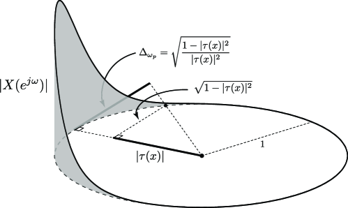
Figure 1: $X(e^{j\omega})$ is a periodic function defined on the unit circle. The figure shows the correspondence between $\tau(x)$ and the periodic frequency spread of the signal.

domain	center	spread
time	$\mu_{n}=\frac{1}{\left\|x\right\|^{2}}\sum_{k\in\mathbb{Z}}k|x_{k}|^{2}$	$\Delta_{n}^{2}=\frac{1}{\left\|x\right\|^{2}}\sum_{k\in\mathbb{Z}}(k-\mu_{n})^{2}|x_{k}|^{2}$
frequency	$\mu_{{\omega}_{p}}=1-\tau(x)\quad\quad$	$\Delta_{{\omega}_{p}}^{2}=\frac{1-\left\lvert\tau(x)\right\rvert^{2}}{\left\lvert\tau(x)\right\rvert^{2}}=\left|\frac{\left\|x\right\|^{2}}{\sum_{k\in\mathbb{Z}}x_{k}\,x_{k+1}^{*}}\right|^{2}-1$

Table 3: Time and frequency centers and spreads for a discrete time signal $x_{n}$ using circular moments, where $\tau(x)$ is defined in (4).

1.2 Contribution

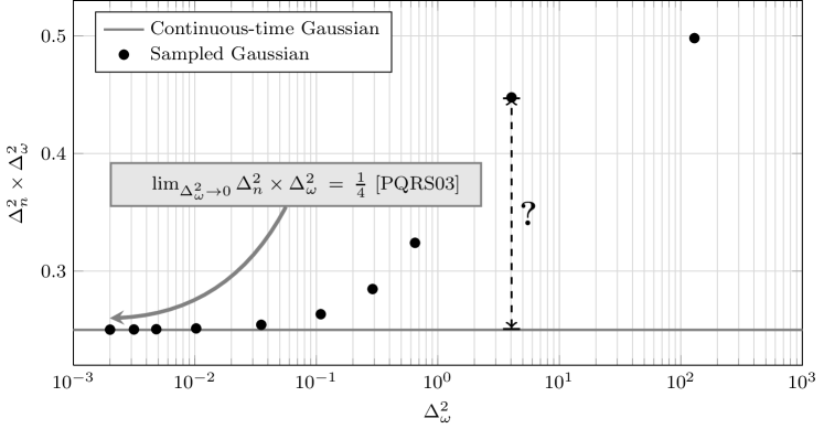
Figure 2: Time-frequency spread of continuous vs. sampled Gaussians. The solid line shows the $1/4$ Heisenberg bound which is achieved by continuous Gaussian signals (with definitions in Table 1), while the markers show the time-frequency spread (according to Table 3) of sampled Gaussian sequences. The question is if the gap between the two curves is inherited from the properties of sequences or sampled Gaussians are not optimal in discrete domain.

In this paper, using the definitions in Table 3, we revisit the Heisenberg uncertainty principle for discrete-time signals. We address the fundamental yet unanswered question: If someone asks us to design a discrete filter with a certain frequency spread ($\Delta_{{\omega}_{p}}^{2}$ fixed), can we return the sequence with minimal time spread $\Delta_{n}^{2}$? In other words, the problem is to find the solution to

$$\Delta_{n,\text{opt}}^{2}\ = \underset{x_{n}}{\text{minimize}} \Delta_{n}^{2}$$ (7)

subject to $$\Delta_{{\omega}_{p}}^{2}\ =\ \sigma^{2}(\text{fixed})\,.$$

In order to provide an insight on the uncertainty principle in the discrete-time domain, we do a simple test. In Figure 2 we show the time-frequency spread of continuous Gaussian signals by the solid line on $1/4$. This is the Heisenberg’s uncertainty bound which is achievable by continuous-time Gaussians. Further, using the definitions in Table 3, we compute the time-frequency spread of sampled Gaussian sequences. According to Prestin et al. [26], the time-frequency spread tends to $1/4$ as the frequency spread of Gaussians decreases. However, when the frequency spread is large, the values are far from the uncertainty bound. Two questions arise here; is the $1/4$ uncertainty bound also tight for discrete sequences? and are sampled Gaussians the minimizers of the uncertainty in the discrete domain? Answers to these questions will be apparent if we can solve (7).

Definition 3.

We call the solution of (7) a maximally compact sequence.

Framing the design of maximally compact sequences as an optimization problem, we show that contrary to the continuous case, it is not possible to reach a constant time-frequency lower bound for arbitrary time or frequency spreads. We further develop a simple optimization framework to find maximally compact sequences in the time domain for a given frequency spread. In other words, we provide in a constructive and numerical way, a sharp uncertainty principle for sequences, later shown in Figure 6. We also show that the Fourier spectra of maximally compact sequences are in fact a very special class of Mathieu’s functions. Using the asymptotical expansion of these functions, we develop closed-form bounds on the time-frequency spread of maximally compact sequences.

1.3 Related Work

The classic uncertainty principle [13] assumes continuous-time non-periodic signals. Several works in the signal processing community also address the discrete-time/discrete-frequency case [19, 6, 24, 20, 15, 11]. Our work bridges these two cases by considering the discrete-time/continuous-frequency regime.

Note that not all studies about the uncertainty principle concern the notion of spread. For example, the authors in [24] propose the uncertainty bound on the information content of signals (entropy) and [6] provides a bound on the non-zero coefficients of discrete-time sequences and their discrete Fourier transforms.

The discrete-time/continuous-frequency scenario has been recently encountered in many practical applications in signal processing. Examples include uncertainty principle on graphs [1], on spheres [14], and on Riemannian manifolds [8]. Studies on the periodic frequency spread can be found in [4] and [35]. The most comprehensive work on the uncertainty relations for discrete sequences is found in [26]. The authors show that $1/4$ is a lower-bound on the time-frequency spread, which can only be achieved asymptotically as the sequence spreads in time. We provide sharp achievable bounds in the non-extreme case which match the results in [26] in the asymptotic regime.

This problem is similar to—although different than—the design of Slepian’s Discrete Prolate Spheroidal Sequences (DPSS’s). First introduced by Slepian in 1978 [30], DPSS’s are sequences designed to be both limited in the time and band-limited in the frequency domains. For a finite length, $N$ in time and a cut-off frequency $W$, the DPSS’s are a collection of $N$ discrete-time sequences that are strictly band-limited to the digital frequency range $|f|<W$, yet highly concentrated in time to the index range $n=0,1,\cdots,N-1$. Such sequences can be found using an algorithm similar to the Papoulis-Gerchberg method. Note the difference of such sequences to the ones that we intend to design in our work; we do not impose any constraints on the bandwidth of the sequences in the frequency domain. Also, the ideas presented here are applicable both to finite and infinite length sequences. Moreover, we focus on the concentration of the signals in the time and frequency domain using the notion of variance.

2 Main Results

The following theorem is the core of the results presented in this paper.

Theorem 1.

For finding unit norm maximally compact sequences, it is sufficient to solve the following semi-definite program (SDP)

$$\underset{\bm{X}}{\text{minimize}} \text{tr}(\bm{T}\bm{X})$$ (8)

subject to $$\text{tr}(\bm{J}_{0}\bm{X})=\alpha$$

$$\text{tr}(\bm{X})=1,\ \ \bm{X}\succeq 0\,,$$

where $\alpha=\frac{1}{\sqrt{1+\sigma^{2}}}$ with $\sigma^{2}$ the fixed periodic frequency spread. Further, $\bm{X}^{\text{opt}}$, the solution to (8) has rank one and $\bm{X}^{\text{opt}}=\bm{x}^{\text{opt}}\ {\bm{x}^{\text{opt}}}^{T}$, with $\bm{x}^{\text{opt}}$ the solution of (7). Matrices $\bm{T}$ and $\bm{J}_{0}$ are defined as

$$\bm{T}={\begin{bmatrix}\ddots&&&&&&\bm{0}\\ &2^{2}&&&&&\\ &&1^{2}&&&&\\ &&&0&&&\\ &&&&1^{2}&&\\ &&&&&2^{2}&\\ \bm{0}&&&&&&\ddots\end{bmatrix}},\quad\quad\bm{J}_{0}=\begin{bmatrix}[1.5]\ddots&\ddots&&&\bm{0}\\ \ddots&0&\frac{1}{2}&&\\ &\frac{1}{2}&0&\frac{1}{2}&\\ &&\frac{1}{2}&0&\ddots\\ \bm{0}&&&\ddots&\ddots\end{bmatrix}\,.$$ (9)

Proof.

See Section 3.2.∎

Remark 1.

The SDP (8) is feasible; indeed we can always find a signal $\bm{x}$ with a certain frequency spread and norm one. Using this signal we can construct $\bm{X}=\bm{x}\bm{x}^{T}$ which shows the feasibility of this problem.

The SDP in (8) can be solved to an arbitrary precision by using existing approaches in the optimization literature; for example using the cvx software package [10]. This gives a constructive way to design sequences that are maximally compact in the time domain with a given frequency spread.

Example 2.

Take $\sigma^{2}=0.1$ to be the fixed and given frequency spread of the sequence. We can use cvx [10] to solve the semi-definite program (8) and find the optimal value of $\Delta_{n}^{2}=2.62$. This results in the time-frequency spread of ${\eta_{p}}=0.262$. The simple code in MATLAB is:

cvx_begin
variable X(n,n);
minimize(trace(T*X))
subject to
    trace(J0*X) == 1/sqrt(1+0.1)
    trace(X) == 1
    X == semi-definite(n)
cvx_end;

Note that contrary to continuous-time signals, we cannot reach the $0.25$ lower bound for sequences. The resulting sequence and its DTFT are shown in Figure 3.

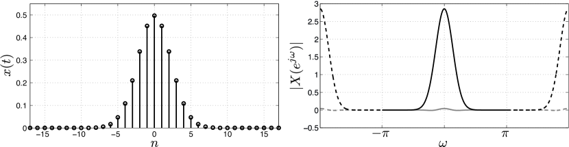
Figure 3: An example solution of (8). The output of the SDP in (8) with $\sigma^{2}=0.1$ using cvx in Example 2. The gray curve in the frequency domain shows the difference from a fitted periodic Gaussian signal. The optimal value for $\Delta_{n}^{2}$ is found to be $2.62$ which results in a time-frequency spread of ${\eta_{p}}=0.262$.

Note that the dual of the SDP (8) is [5, p. 265]:

$$\underset{\lambda_{1},\lambda_{2}}{\text{maximize}} \alpha\,\lambda_{1}+\lambda_{2}$$ (10)

subject to $$\bm{T}-\lambda_{1}\,\bm{J}_{0}-\lambda_{2}\,\bm{I}\succeq 0\,.$$

We will use the formulation of the dual problem many times in the rest of the paper.

Lemma 1.

For maximally compact sequences, $\Delta_{n}^{2}(x)$ changes monotonically with $\Delta_{{\omega}_{p}}^{2}(x)$.

Proof.

The feasible region of the dual (10) is shown in Figure 4. We can write (10) as

$$\underset{\lambda_{1},\lambda_{2}}{\text{maximize}} c$$ (11)

subject to $$\lambda_{2}=c-\alpha\,\lambda_{1}\,,$$

$$\bm{T}-\lambda_{1}\,\bm{J}_{0}-\lambda_{2}\,\bm{I}\succeq 0\,.$$

Note that $\alpha$ changes between $0$ and $1$ (see Figure 4). For a fixed $\alpha$, the maximum $c^{\text{opt}}$ is found by elevating the corresponding line $\lambda_{2}=c-\alpha\lambda_{1}$ until it supports the feasible set (it is tangent to it). Since the feasible set is convex, as $\alpha$ grows (which means $\Delta_{{\omega}_{p}}^{2}$ decreases), we need a higher elevation of the line to support the convex set, thus $c^{\text{opt}}$ (equivalently $\Delta_{n}^{2}$) increases. This phenomenon is later confirmed by the simulation results in Figure 6.

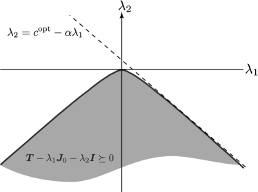
Figure 4: The feasible set of the dual problem (10) and the supporting line. As $\alpha$ increases, we need to elevate the line more to support the feasible set, which means that the optimal value of $\Delta_{n}^{2}$ increases.

∎

Although Theorem 1 provides a constructive way for finding maximally compact sequences, it does not specify the closed form for these sequences. One would be interested to see if—in analogy to continuous-time—sampled gaussians are maximally compact? The answer is negative, as shown by the following theorem:

Theorem 2.

The DTFT spectra, $X(e^{j\omega})$ of maximally compact sequences are Mathieu’s functions. More specifically,

$$X(e^{j{\omega}})\>=\>\gamma_{0}\cdot{\mathrm{ce}}_{0}(-2\lambda_{1}\>;\>({\omega}-{\omega}_{0})/2)e^{j\mu{\omega}}\ ,$$ (12)

where $|\gamma_{0}|=\|{\mathrm{ce}}_{0}(-2\lambda_{1}\>;\>({\omega}-{\omega}_{0})/2)\|^{-1}$, ${\omega}_{0}$ and $\mu$ are shifts in frequency or time and $\lambda_{1}$ is the optimal solution of the dual problem (10). ${\mathrm{ce}}_{0}(q\ ;{\omega})$ is Mathieu’s harmonic cosine function of order zero.

Mathieu’s functions—widely used in quantum mechanics [33]—are the solutions to Mathieu’s differential equation [2, §20.1.1]:

$$\frac{\partial^{2}y(\omega)}{\partial\omega^{2}}+(a-2q\cos(2\omega))\cdot y(\omega)\>=\>0\,.$$ (13)

These functions assume an even (Mathieu’s cosine function) and odd form (Mathieu’s sine function). For some specific pairs $(a,q)$, Mathieu’s functions can be restricted to be $2\pi$ periodic. Mathieu’s harmonic Cosine functions of order $m$ are thus:

$${\mathrm{ce}}_{m}(q\>;\>{\omega})\>=\>{\mathrm{ce}}(a_{m}(q),q\>;\>{\omega}),\ m\in\mathbb{N}.$$ (14)

For the proof of Theorem 2 and further insights on Mathieu’s functions, we refer the reader to Section 3.3.

Using the constructive method presented in Theorem 1, we can find the achievable (and tight) uncertainty principle bound for discrete sequences. This is shown and discussed more in Section 5 and Figure 6. However, a numerically computed boundary may not always be practical, and even though the numerical solution exactly solves the problem, its accuracy may be challenged. Therefore, we characterize the asymptotic behavior of the time-frequency bound:

Theorem 3.

If $x_{n}$ is maximally compact for a given $\Delta_{{\omega}_{p}}^{2}=\sigma^{2}$, then

$$\eta_{p}=\Delta_{n}^{2}\ \Delta_{{\omega}_{p}}^{2}\geq\sigma^{2}\left(1-\sqrt{\frac{\sigma^{2}}{1+\sigma^{2}}}\right)\,.$$ (15)

Further, for small values of $\sigma^{2}$, maximally compact sequences satisfy

$$\eta_{p}=\Delta_{n}^{2}\ \Delta_{{\omega}_{p}}^{2}\leq\frac{\sigma^{2}}{8}\left(\frac{\sqrt{1+\sigma^{2}}}{\sqrt{1+\sigma^{2}}-1}-\frac{1}{2}\right)\,.$$ (16)

Proof.

The proof for this theorem is provided in Section 4. ∎

This fundamental result states that for a given frequency spread, we cannot design sequences which achieve the classic Heisenberg uncertainty bound. We will see how this curve compares to the classic Heisenberg bound in Section 5.

The lower bound in (15) converges to $1/2$ as the value of $\sigma^{2}$ grows, and “pushes up” the time-frequency spread of maximally compact sequences towards $1/2$ which is also an asymptotic upper bound on the time-frequency spread as $\Delta_{{\omega}_{p}}^{2}\rightarrow\infty$; indeed, one may construct the unit-norm sequence $x^{(\varepsilon)}_{n}=\varepsilon\ \delta_{n+1}+\sqrt{1-2\varepsilon^{2}}\ \delta_{n}+\varepsilon\ \delta_{n-1}$, which verifies $\lim_{\varepsilon\rightarrow 0}\eta_{p}(x^{(\varepsilon)})=1/2$.

On the other hand, for small values of $\sigma^{2}$, the upper bound in (16) converges from above to $1/4$, thus “pushing down” the time-frequency spread of maximally compact sequences towards the Heisenberg uncertainty bound $1/4$ from above.

2.0.1 Finite-Length Sequences

The theory that we have provided so far holds for infinite sequences. For computational purposes, we have to assume finite length for the sequences in the time domain, which is not an issue if the sequence length is chosen to be long enough. As a side benefit, a length constraint on the sequence may be added without changing the design algorithm.

3 Proof of Theorems 1 and 2

Let us start with some properties of maximally compact sequences.

3.1 Properties of Maximally Compact Sequences

In the definitions of time and frequency spreads in Table 3 we considered complex sequences and their DTFTs. In the following, we establish two lemmas that make the search for maximally compact sequences easier. In the first lemma (Lemma 2), we state that if someone gives us a complex sequence with a given time-frequency spread, we can always take the modulus and have a sequence with a smaller or equal time-frequency spread. This enables us to only consider real sequences as maximally compact sequences. In Lemma 3, we state that shifts in time do not affect the time-frequency spread of sequences. This lemma allows us to assume—without loss of generality—that the sequences are centered around zero in time.

Lemma 2.

For any given sequence $x_{k}$,

$$\eta_{p}(\left\lvert x\right\rvert)\leq\eta_{p}(x)\,.$$

Proof.

Let $x_{k}$ be a sequence with a given time spread $\Delta_{n}^{2}(x)$. Obviously,

$$\Delta_{n}^{2}(x)\>=\>\Delta_{n}^{2}(|x|).$$

Moreover,

$$\Delta_{{\omega}_{p}}^{2}(|x|)\>=\> \left|\sum_{k\in\mathbb{Z}}|x_{k}||x_{k+1}|\right|^{-2}-1$$

$$\>\leq\> \left|\sum_{k\in\mathbb{Z}}x_{k}x_{k+1}^{\ast}\right|^{-2}-1\quad\>=\>\Delta_{{\omega}_{p}}^{2}(x).$$

∎

Recall from Lemma 1 that for maximally compact sequences $\Delta_{n}^{2}$ changes monotonically with $\Delta_{{\omega}_{p}}^{2}$. Thus, it is equivalent to fix either one of $\Delta_{n}^{2}$ or $\Delta_{{\omega}_{p}}^{2}$, and optimize with respect to the other.

Lemma 3.

If $x$ is a maximally compact sequence, then $x_{k-\mu_{n}(x)}$ is also maximally compact. For non-integer $\mu_{n}$, $x_{k-{\mu_{n}}}$ is a shorthand for sinc resampling on a grid shifted by $\mu_{n}$ in the time domain.

Proof.

As $\mu_{n}$ is not necessarily an integer, we can use the Parseval’s equality to show that the time center and spread is not affected by arbitrary shifts. These easy computations are left to the interested reader (They can be found in [22]). Thus, if $x$ is a maximally compact sequence, then $x_{k-\mu_{n}(x)}$ is also maximally compact (note that time shift does not change the frequency characteristics of the sequence).

∎

Remark 2.

Using Lemmas 2 and 3, we only consider real sequences $x$, with $\mu_{n}(x)=0$ and $\|x\|_{2}=1$. Later in Theorem 2 we show that maximally compact sequences are Mathieu’s cosine functions, which have strictly positive inverse Fourier transforms. This enables us to state that maximally compact sequences are real sequences up to a shift, scale or modulation.

3.2 Proof of Theorem 1

By using Lemmas 2 and 3, we can write problem (7) as

$$\Delta_{n,\text{opt}}^{2}\ = \underset{x_{n}}{\text{minimize}} \sum_{k\in\mathbb{Z}}k^{2}x_{k}^{2}$$ (17)

subject to $$\sum_{k\in\mathbb{Z}}x_{k}x_{k+1}=\frac{1}{\sqrt{1+\sigma^{2}}},$$

$$\sum_{k\in\mathbb{Z}}x_{k}^{2}=1.$$

We can rewrite (17) in matrix form as a quadratically constrained quadratic program (QCQP) [5, p. 152]:

$$\begin{aligned} &\underset{\bm{x}}{\text{minimize}}&&\bm{x}^{T}\bm{T}\bm{x}\\ &\text{subject to}&&\bm{x}^{T}\bm{J}_{0}\bm{x}=\alpha\,,\\ &&&\bm{x}^{T}\bm{x}=1\,,\end{aligned}\quad\quad\quad\quad\equiv\quad\quad\quad\quad\begin{aligned} &\underset{\bm{x}}{\text{minimize}}&&\text{tr}(\bm{T}\bm{x}\bm{x}^{T})\\ &\text{subject to}&&\text{tr}(\bm{J}_{0}\bm{x}\bm{x}^{T})=\alpha\\ &&&\text{tr}(\bm{x}\bm{x}^{T})=1\,.\end{aligned}$$ (18)

where $\bm{T}$ and $\bm{J}_{0}$ are defined in (9) and $\alpha=1/\sqrt{1+\sigma^{2}}$. Replacing $\bm{x}\bm{x}^{T}$ by $\bm{X}$, we can write equivalently

$$\underset{\bm{X}}{\text{minimize}} \text{tr}(\bm{T}\bm{X})$$ (19)

subject to $$\text{tr}(\bm{J}_{0}\bm{X})=\alpha$$

$$\text{tr}(\bm{X})=1$$

$$\bm{X}\succeq 0,\;\text{rank}(\bm{X})=1\,.$$

We further relax the above formulation to reach the semi-definite program

$$\underset{\bm{X}}{\text{minimize}} \text{tr}(\bm{T}\bm{X})$$ (20)

subject to $$\text{tr}(\bm{J}_{0}\bm{X})=\alpha$$

$$\text{tr}(\bm{X})=1,\ \ \bm{X}\succeq 0\,.$$

In Lemma 4 we show that the semi-definite relaxation is tight. This finishes the proof for Theorem 1. ∎

Lemma 4.

The semi-definite relaxation (SDR) from (19) to (20) is tight.

Proof.

Shapiro and then Barnivok and Pataki [29, 3, 23, 16] show that if the SDP in (19) is feasible, then

$$\text{rank}(\bm{X}^{\mathrm{opt}})\leq\lfloor(\sqrt{8m+1}-1)/2\rfloor\,,$$ (21)

where $m$ is the number of constraints of the SDP and $\bm{X}^{\mathrm{opt}}$ is its optimal solution. For our semi-definite program in (20), $m=2$. Thus, (21) implies that the solution has rank 1. Using this fact, one can see that the semi-definite relaxation is in fact tight. Recall from Remark 1 that problem (8) (and also (19)) is feasible. ∎

3.3 Proof of Theorem 2

We start by problem (8) and its dual (10).

Lemma 5.

For the primal problem (8) and the dual (10), strong duality holds.

Proof.

For a semi-definite program and its dual, if the primal is feasible and the dual is strictly feasible, then strong duality holds [31, 32] .

We saw in Remark 1 that the primal problem (8) is feasible. For the dual, one can use the Gershgorin’s circle theorem and show that a sufficient condition for $\bm{T}-\lambda_{1}\,\bm{J}_{0}-\lambda_{2}\,\bm{I}\succ 0$ to hold is $\lambda_{2}<-\lambda_{1}$ and $\lambda_{1}>0$. Thus, the dual problem is strictly feasible. ∎

Thus, for finding the time-frequency spread of maximally compact sequences, solving the dual problem suffices. If a sequence is a solution to the dual SDP problem (10), the dual constraint is active. Therefore, maximally compact sequences lie on the boundary of the quadratic cone

$$\bm{T}-\lambda_{1}\,\bm{J}_{0}-\lambda_{2}\,\bm{I}\succeq 0.$$

A maximally compact sequence $\bm{x}$ is thus solution of the eigenvalue problem

$$(\bm{T}-\lambda_{1}\,\bm{J}_{0})\bm{x}\>=\>\lambda_{2}\,\bm{x},$$ (22)

where $\lambda_{1}$ and $\lambda_{2}$ are the dual variables of the SDP problem. $\lambda_{2}$ is also the minimal eigenvalue of $\bm{T}-\lambda_{1}\,\bm{J}_{0}$ with $\bm{x}$ the associated eigenvector (this can be also seen by forcing the derivative of the Lagrangian in (18) to zero).

This explicit link between the dual variables and the sequence, yields a differential equation for which the DTFT spectrum of maximally compact sequences is the solution. In the DTFT domain (22) becomes (expanding the matrix multiplications)

$$X^{\prime\prime}(e^{j{\omega}})+\left(\lambda_{2}+\lambda_{1}\cos({\omega})\right)X(e^{j{\omega}})\>=\>0\>,$$ (23)

which is Mathieu’s differential equation (13). Taking into account the periodicity of (23), it appears that not all pairs of parameters $(a,q)$ will lead to a periodic solution. Mathieu’s functions can be restricted to be $2\pi$ periodic. The solutions of Mathieu’s harmonic differential equation—equation (13) with a $2\pi$-periodic solution $y$—are defined as

Mathieu’s harmonic Cosine (even, periodic) $${\mathrm{ce}}_{m}(q\>;\>{\omega})\>=\>{\mathrm{ce}}(a_{m}(q),q\>;\>{\omega})\ ,\ m\in\mathbb{N}.$$ (24)

Mathieu’s harmonic Sine (odd, periodic) $${\mathrm{se}}_{m}(q\>;\>{\omega})\>=\>{\mathrm{ce}}(b_{m}(q),q\>;\>{\omega})\ ,\ m\in\mathbb{N}^{+}.$$ (25)

It is immediately visible that the spectrum of maximally compact sequences may only have the form

$$X(e^{j{\omega}})\>=\>\begin{cases}\gamma_{0}\,{\mathrm{ce}}_{m}(-2\lambda_{1}\>;\>{\omega}/2)+\gamma_{1}\,{\mathrm{se}}_{m}(-2\lambda_{1}\>;\>{\omega}/2)&\text{ for }m\in\mathbb{N}^{+},\\ \gamma_{0}\,{\mathrm{ce}}_{m}(-2\lambda_{1}\>;\>{\omega}/2)&\text{ for }m=0\>,\end{cases}$$ (26)

for any constants $\gamma_{0}$ and $\gamma_{1}$ such that $\|X(e^{j{\omega}})\|=2\pi$. More specifically, for any $\lambda_{1}\geq 0$, the dual SDP problem can be posed and any solution would have the form (26).

Charasteristic numbers of Mathieu’s equation are ordered [7, p. 113], such that for $\lambda_{1}>0$,

$$\begin{array}[]{rl}a_{0}(-2\lambda_{1})<a_{1}(-2\lambda_{1})<b_{1}(-2\lambda_{1})<b_{2}(-2\lambda_{1})<a_{2}(-2\lambda_{1})<\cdots\,.\end{array}$$

By (13) and with the substitution ${\omega}\rightarrow{\omega}/2$ one obtains $a_{m}(-2\lambda_{1})=4\lambda_{2}$. Because $\lambda_{2}$ is the minimal eigenvalue, we conclude that $m=0$.

Note that this result validates the one in [12] which stated that asymptotically Mathieu’s functions minimize the time-frequency product. With a diferent approach, we can establish that only Mathieu’s harmonic cosine of order 0 minimizes this product for any given frequency-spread.

4 Proof of Theorem 3

Let us start by proving the lower bound.

4.1 Lower Bound (15)

In order to prove the lower bound (15) we first provide the following two lemmas.

Lemma 6.

Consider the sequence $a_{k}$ as follows with $\theta,\nu>0$

$$a_{k+1}=(k+1)^{2}+\theta-\frac{\nu}{a_{k}}\,.$$ (27)

The sequence $a_{k}$ is positive for $k\geq k_{0}$ as soon as $a_{k_{0}+1}\geq a_{k_{0}}>0$.

Proof.

Note that

$$a_{k+2}-a_{k+1} =3+2k+\nu\frac{a_{k+1}-a_{k}}{a_{k+1}a_{k}}\,.$$ (28)

Thus, by induction, the sequence is positive as soon as $a_{k_{0}+1}\geq a_{k_{0}}>0$ for some $k_{0}$. ∎

Lemma 7.

If

$$\lambda_{2}<1-\sqrt{1+\lambda_{1}^{2}}\,,$$ (29)

then ${\bm{P}}=\bm{T}-\lambda_{1}\,\bm{J}_{0}-\lambda_{2}\,\bm{I}\succeq 0$.

Proof.

Note that if $\lambda_{1}=0$, then the matrix ${\bm{P}}$ is positive-definite with the given condition. In the proof we will thus assume that $\lambda_{1}\neq 0$.

Consider the following tri-diagonal matrices ${\bm{P}}_{1}$ and ${\bm{P}}_{2}$:

$${\bm{P}}_{1}=\begin{bmatrix}[1.5]1-\lambda_{2}&-\lambda_{1}/2&&\bm{0}\\ -\lambda_{1}/2&4-\lambda_{2}&-\lambda_{1}/2&\\ &-\lambda_{1}/2&9-\lambda_{2}&\ddots\\ \bm{0}&&\ddots&\ddots\end{bmatrix},\,\quad{\bm{P}}_{2}=\begin{bmatrix}[1.5]0-\lambda_{2}&-\lambda_{1}&&\bm{0}\\ -\lambda_{1}/2&1-\lambda_{2}&-\lambda_{1}/2&\\ &-\lambda_{1}/2&4-\lambda_{2}&\ddots\\ \bm{0}&&\ddots&\ddots\end{bmatrix}\,.$$ (30)

Call $\mathcal{I}$ the set of eigenvalues of ${\bm{P}}$, $\mathcal{I}_{1}$ the set of eigenvalues of ${\bm{P}}_{1}$ and $\mathcal{I}_{2}$ the set of eigenvalues of ${\bm{P}}_{2}$. It is trivial to see that $\mathcal{I}=\mathcal{I}_{1}\cup\mathcal{I}_{2}$.

We show that if condition (29) is satisfied, then both ${\bm{P}}_{1}$ and ${\bm{P}}_{2}$ have positive eigenvalues.

1. ${\bm{P}}_{1}$: Sylvester’s criterion states that a symmetric matrix is positive definite if and only if its principal minors are all positive. As ${\bm{P}}_{1}$ is symmetric, we can use Sylvester’s criterion on it. We use Gaussian elimination on the matrix ${\bm{P}}_{1}$ to compute its principal minors

   $${{\bm{P}}}_{1}^{\text{U}}=\begin{bmatrix}[1.5]1-\lambda_{2}&-\lambda_{1}/2&&&\bm{0}\\ 0&s_{2}&-\lambda_{1}/2&&\\ &0&s_{3}&-\lambda_{1}/2&\\ \bm{0}&&0&\ddots&\ddots\end{bmatrix}\,,$$ (31)

   where

   $$s_{k+1}=(k+1)^{2}-\lambda_{2}-\frac{\lambda_{1}^{2}}{4s_{k}}\,,\quad k\geq 1\,.$$

   This satisfies the induction formula in (27). Thus according to Lemma 6, the principal minors of ${{\bm{P}}}_{1}^{\text{U}}$ (and so ${\bm{P}}_{1}$) are positive as soon as $s_{2}\geq s_{1}>0$. This is equivalent to $1-\lambda_{2}>0$ and $4-\lambda_{2}-\frac{\lambda_{1}^{2}}{4(1-\lambda_{2})}\geq 1-\lambda_{2}$. i.e., $\lambda_{1}^{2}\leq 12(1-\lambda_{2})$, which is a weaker condition than (29). Therefore, ${\bm{P}}_{1}$ is also positive semi-definite.

    

2. ${\bm{P}}_{2}$: We can decompose ${\bm{P}}_{2}$ as

   $${\bm{P}}_{2}=\begin{bmatrix}2&&&&\bm{0}\\ &1&&&\\ &&1&&\\ \bm{0}&&&&\ddots\\ \end{bmatrix}\times\begin{bmatrix}[1.5]0-\lambda_{2}/2&-\lambda_{1}/2&&\bm{0}\\ -\lambda_{1}/2&1-\lambda_{2}&-\lambda_{1}/2&\\ &-\lambda_{1}/2&4-\lambda_{2}&\ddots\\ \bm{0}&&\ddots&\ddots\end{bmatrix}\ =\ \bm{D}\times{\bm{P}}_{2}^{\text{(s)}}\ .$$ (32)

   Note that both $\bm{D}$ and ${\bm{P}}_{2}^{\text{(s)}}$ are symmetric. Also observe that the eigenvalues of ${\bm{P}}_{2}$ and ${\bm{P}}_{2}^{\text{(s)}}$ are equal. Thus, it suffices to consider the eigenvalues of ${\bm{P}}_{2}^{\text{(s)}}$; If ${\bm{P}}_{2}^{\text{(s)}}$ is positive-definite then all the eigenvalues of ${\bm{P}}_{2}$ are positive.

   Again using Gaussian elimination on ${\bm{P}}_{2}^{\text{(s)}}$ results in

   $${\bm{P}}_{2}^{\text{(s),U}}=\begin{bmatrix}[1.5]-\lambda_{2}/2&-\lambda_{1}/2&0&&\bm{0}\\ 0&s_{1}&-\lambda_{1}/2&&\\ &0&s_{2}&-\lambda_{1}/2&\\ \bm{0}&&0&\ddots&\ddots\end{bmatrix}\,,$$ (33)

   where $s_{1}=1-\lambda_{2}+\lambda_{1}^{2}/2\lambda_{2}$ and $s_{k}$ has the following form $s_{k+1}=(k+1)^{2}-\lambda_{2}-\frac{\lambda_{1}^{2}}{4s_{k}}\,,\quad k\geq 1$. This again satisfies the induction formula (27). Therefore, it suffices to show that $\lambda_{2}<0$ and $s_{2}\geq s_{1}>0$. We show that under condition (29), this is true. In order to satisfy $s_{1}>0$, we need $1-\lambda_{2}+\lambda_{1}^{2}/2\lambda_{2}>0$, which is equivalent to $\lambda_{2}<\frac{1}{2}(1-\sqrt{1+2\lambda_{2}^{2}})$. This is a weaker condition than (29).

   Further, in order to satisfy $s_{2}>s_{1}$, we need

   $$s_{2}-s_{1}=3+\frac{\lambda_{1}^{2}}{4s_{1}\lambda_{2}^{2}}(\lambda_{2}^{2}-2\lambda_{2}-\lambda_{1}^{2})\geq 0\,.$$

   Thus, it is enough to have $\lambda_{2}^{2}-2\lambda_{2}-\lambda_{1}^{2}\geq 0$. That is $\lambda_{2}\leq 1-\sqrt{1+\lambda_{1}^{2}}$, which is the bound provided in (29). Putting these together, we can conclude that under condition (29), the matrix ${\bm{P}}$ is positive-definite.

∎

Note that condition (29) gives a sufficient (but not necessary) condition on the feasible set of the dual problem (10). Thus, it provides a lower bound for the maximum value of the dual. Consider the restricted dual problem

$$\underset{\lambda_{1},\lambda_{2}}{\text{maximize}} \alpha\,\lambda_{1}+\lambda_{2}$$ (34)

subject to $$\lambda_{2}<1-\sqrt{1+\lambda_{1}^{2}}$$

The solution to this problem is simply $1-\sqrt{1-\alpha^{2}}$. If we rewrite $\alpha$ in terms of $\sigma^{2}$, we finally have

$$\Delta_{n,\text{opt}}^{2}\geq 1-\sqrt{\frac{\sigma^{2}}{1+\sigma^{2}}}\,.$$

This concludes the proof for the lower bound.

4.2 Upper Bound (16)

It is easy to see that for small values of $\sigma^{2}$ (equivalently $\alpha$ closer to $1$), the maximum of the dual problem is achieved for large values of $\lambda_{1}$ (remember that $\lambda_{1}$ needs to be positive). We saw in 3.3 that for maximally compact sequences (i.e. sequences that result in the maximum of the dual problem) we have $\lambda_{2}=1/4\ a_{0}(2\lambda_{1})$ (note that $a_{0}(-q)=a_{0}(q)$). McLachlan in [17] shows that for large enough values of $q$, we have

$$a_{0}(q) =-2q+2q^{\frac{1}{2}}-\frac{1}{4}-\frac{1}{32}q^{\frac{-1}{2}}-\frac{48}{2^{7}}q^{-1}-\frac{848}{2^{17}}q^{\frac{-3}{2}}-\frac{4,752}{2^{20}}q^{-2}-\frac{126,752}{2^{20}}q^{\frac{-5}{2}}-\cdots$$ (35)

$$=-2q+2q^{\frac{1}{2}}-\frac{1}{4}-\frac{1}{32}q^{\frac{-1}{2}}+O(q^{-1})\,.$$

Thus, we have for large $q$,

$$a_{0}(q)\leq-2q+2q^{\frac{1}{2}}-\frac{1}{4}\,.$$ (36)

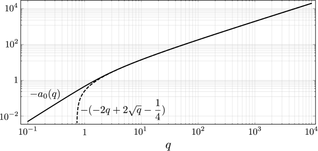
Figure 5: The characteristic number $a_{0}(q)$ of Mathieu’s function together with its upper bound. In order to plot on a log scale, the negations are plotted.

The values for $a_{0}(q)$ and its upper bound are shown in Figure 5. In order to be able to plot on a log scale, their negative counterparts are plotted.

After replacing $q$ by $2\lambda_{1}$ and $a_{0}(2\lambda)$ by $4\lambda_{2}$ in (36), we have

$$\lambda_{2}=\frac{1}{4}a_{0}(2\lambda_{1})\leq-\lambda_{1}+\frac{1}{\sqrt{2}}\sqrt{\lambda_{1}}-\frac{1}{16}\,.$$ (37)

Because this set contains the original feasible set of the dual problem, it will give an upper bound on the optimal value of the dual. In other words, $\Delta_{n}^{2}\leq\sigma_{r}^{2}$, where

$$\sigma_{r}^{2}\>= \underset{\lambda_{1},\lambda_{2}}{\text{maximize}} \alpha\,\lambda_{1}+\lambda_{2}$$ (38)

subject to $$\lambda_{2}\leq-\lambda_{1}+\frac{1}{\sqrt{2}}\sqrt{\lambda_{1}}-\frac{1}{16}\,.$$

It is easy to see that the maximum of (38) is achieved for $\lambda_{1}=\frac{1}{8(1-\alpha)^{2}}$. Replacing $\lambda_{1}$ in (38) and using the fact that $\Delta_{n,\text{opt}}^{2}\leq\sigma_{r}^{2}$, leads to

$$\Delta_{n,\text{opt}}^{2}\leq\frac{1}{8}\left(\frac{\sqrt{1+\sigma^{2}}}{\sqrt{1+\sigma^{2}}-1}-\frac{1}{2}\right)\,.$$ (39)

5 Simulation Results

In order to show the behaviour of the results obtained in Theorems 1 and 3, we ran some simulations. For this, we assumed that the designed filter is finite length with 201 taps in the time domain. The length is long enough not to pose restrictions on the solution for the considered frequency spreads. For smaller frequency spreads, we can increase the length of the sequence. For different values of $\Delta_{{\omega}_{p}}^{2}\>=\>\sigma^{2}$, we solved the semi-definite program (8) using the cvx toolbox in MATLAB.

The resulting values of $\Delta_{n}^{2}$ were then multiplied with the corresponding $\Delta_{{\omega}_{p}}^{2}$ to produce the time-frequency spread of maximally compact sequences. The time-frequency spread of maximally compact sequences versus their frequency spread is shown with the solid curve in Figure 6. This means—numerically—that any time-frequency spread under this curve is not achievable. The dotted line in this figure shows the classic Heisenberg uncertainty bound. Comparing the two curves shows the gap between the classic Heisenberg principle and what is achievable in practice. The dashed lines represent analytical lower and upper bounds for the time-frequency spread of maximally compact sequences (found in Theorem 3).

[width=1]figs/tfprodAndLB.eps

Figure 6: New uncertainty bounds. The solid line shows the results of solving the SDP in (8). The dotted line shows the classic Heisenberg uncertainty principle. The dashed lines show the analytic lower and upper bounds found in Theorem 3.

Further, to give an insight on how the time-frequency spread of some common filters compare to that of maximally compact sequences, we plot their time-frequency spread together with the new uncertainty bound in Figure 7. By changing the length of each filter in time, we can find its time and frequency spreads which results in a point on the figure. We observe that as shown by Prestin et al. in [26], asymptotically when the frequency spread of sequences are very small, sampled Gaussians converge to the lower bound for maximally compact sequences.

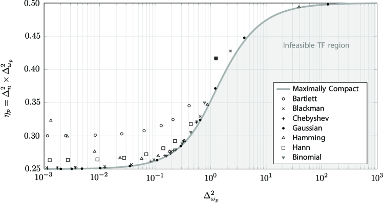
Figure 7: Time-frequency spread of common FIR filters. By changing the length of the filters in time, we compute the time and frequency spreads for each type of filters. For small values of the frequency spread, Gaussian filters are good approximations of Mathieu’s functions (as shown also in [26]).

6 Conclusion

We showed that for discrete-time sequences, contrary to continuous-time signals, the classic Heisenberg uncertainty bound is not always achievable and the uncertainty minimizers have a large gap from this bound. We constructed an optimization framework for finding the uncertainty minimizers which we refer to as the “maximally compact sequences”. This framework allows one to find—numerically and efficiently—the most compact sequence in time with a desired frequency spread. We further showed that the discrete-time Fourier transform of these sequences is a very special class of Mathieu’s functions. We also proved analytic bounds on the time-frequency spread of discrete sequences. Maximally compact sequences can serve as optimal probing windows (similarly to the ones shown in Figure 7) in several signal processing applications. Furthermore, the connection provided between the solutions of the semi-definite program and Mathieu’s functions, also enables the approximation of Mathieu’s functions with arbitrary accuracy.

Ackowledgements

The authors would like to thank Dr. Arash Amini and Dr. Seyed Hamed Hassani for their help in proving Theorem 3, and Ivan Dokmanic for his insight on Mathieu’s functions. The authors would also like to thank the reviewers for their valuable contributions in the improvement of the manuscript, and pointing out a related recent work [21], which was published on arxiv after the submission of this manuscript and during the review process.

References

- AL [12] A. Agaskar and Y.M. Lu. Uncertainty principles for signals defined on graphs: Bounds and characterizations. In ICASSP, pages 3493–3496, 2012.
- AS [72] M. Abramowitz and I.A. Stegun. Handbook of Mathematical Functions with Formulas, Graphs, and Mathematical Tables. National Bureau of Standards Applied Mathematics Series 55. Tenth Printing. ERIC, 1972.
- Bar [95] A.I. Barvinok. Problems of distance geometry and convex properties of quadratic maps. Discrete & Computational Geometry, 13(1):189–202, 1995.
- Bre [85] E. Breitenberger. Uncertainty measures and uncertainty relations for angle observables. Foundations of Physics, 15(3):353–364, 1985.
- BV [04] S. Boyd and L. Vandenberghe. Convex optimization. Cambridge University Press, 2004.
- DS [89] D. L. Donoho and P. B. Stark. Uncertainty principles and signal recovery. SIAM J. Appl. Math., 49(3):906–931, 1989.
- EMO+ [55] A. Erdélyi, W. Magnus, F. Oberhettinger, F. G. Tricomi, and H. Bateman. Higher transcendental functions, volume 3. McGraw-Hill New York, 1955.
- Erb [09] W. Erb. Uncertainty Principles on Riemannian Manifolds. PhD thesis, Tech. Universität München, 2009.
- Gab [46] D. Gabor. Theory of communication. Journal of the Institution of Electrical Engineers, 93(26):429–457, 1946.
- GB [10] M. Grant and S. Boyd. cvx: MATLAB software for disciplined convex programming, version 1.21. http://cvxr.com/cvx, 2010.
- GJ [11] S. Ghobber and P. Jaming. On uncertainty principles in the finite dimensional setting. Linear Algebra and its Applications, 435(4):751–768, 2011.
- GM [02] S. S. Goh and C. A. Micchelli. Uncertainty principles in Hilbert spaces. J. Fourier Anal. Appl., 8:335–374, 2002.
- Hei [27] W. Heisenberg. The actual content of quantum theoretical kinematics and mechanics. Phys. Z., 43:172, 1927.
- KDSK [12] Z. Khalid, S. Durrani, P. Sadeghi, and R.A. Kennedy. Concentration uncertainty principles for signals on the unit sphere. In ICASSP, pages 3717 –3720, march 2012.
- KPR [08] F. Krahmer, G. E. Pfander, and P. Rashkov. Uncertainty in time–frequency representations on finite Abelian groups and applications. Applied and Computational Harmonic Analysis, 25(2):209 – 225, 2008.
- LMS+ [10] Z. Luo, W. Ma, A. M. C. So, Y. Ye, and S. Zhang. Semidefinite relaxation of quadratic optimization problems. IEEE Signal Processing Magazine, 27(3):20–34, 2010.
- Mac [64] N. W. MacLachlan. Theory and Applications of Mathieu Functions, page 232. Dover Publications, 1964.
- MJ [09] K. V. Mardia and P. E. Jupp. Directional Statistics, pages 20–31. Wiley, 2009.
- MS [73] T. Matolcsi and J. Szűcs. Intersection des mesures spectrales conjuguées. R. Acad. Sci., 277:A841–A843, 1973.
- MS [08] S. Massar and Ph. Spindel. Uncertainty relation for the discrete Fourier transform. Phys. Rev. Lett., 100:190401, May 2008.
- Nam [13] S. Nam. An uncertainty principle for discrete signals. CoRR, abs/1307.6321, 2013.
- Par [13] R. Parhizkar. Euclidean Distance Matrices: Properties, Algorithms and Applications. PhD thesis, Ecole Polytechnique Federale de Lausanne (EPFL), 2013.
- Pat [98] G. Pataki. On the rank of extreme matrices in semidefinite programs and the multiplicity of optimal eigenvalues. Mathematics of Operations Research, pages 339–358, 1998.
- PDO [99] T. Przebinda, V. DeBrunner, and M. Ozaydin. Using a new uncertainty measure to determine optimal bases for signal representations. In ICASSP, 1999.
- PQ [99] J. Prestin and E. Quak. Optimal functions for a periodic uncertainty principle and multiresolution analysis. Proceedings of the Edinburgh Mathematical Society, 42(2):225–242, 1999.
- PQRS [03] J. Prestin, E. Quak, H. Rauhut, and K. Selig. On the connection of uncertainty principles for functions on the circle and on the real line. J. Fourier Anal. Appl., 9(4):387–409, 2003.
- Rob [29] H. P. Robertson. The uncertainty principle. Physical Review, 34:163–164, 1929.
- Sch [30] E. Schrödinger. About Heisenberg uncertainty relation. Proc. Prussian Acad. Sci., XIX:296–303, 1930.
- Sha [82] A. Shapiro. Rank-reducibility of a symmetric matrix and sampling theory of minimum trace factor analysis. Psychometrika, 47(2):187–199, 1982.
- Sle [78] D. Slepian. Prolate spheroidal wave functions, Fourier analysis, and uncertainty. V:The discrete case. 57(5):1371–1430, 1978.
- Tod [01] M. J. Todd. Semidefinite optimization. Acta Numerica, 10:515–560, 2001.
- Trn [05] M. Trnovská. Strong duality conditions in semidefinite programming. J. of Elec. Eng., 56(12), 2005.
- UCYG [02] C. I. Um, J. R. Choi, K. H. Yeon, and T. F. George. Exact quantum theory of the harmonic oscillator with the classical solution in the form of mathieu functions. Journal of the Korean Physical Society, 40(6):969–973, 2002.
- VKG [13] M. Vetterli, J. Kovacevic, and V. K. Goyal. Foundations of Signal Processing, chapter 7. 2013. http://www.fourierandwavelets.org/.
- vM [18] R. von Mises. Über die “Ganzzahligkeit” der Atomgewichte und verwandte Fragen. Phys. Z., 19:490–500, 1918.