A mixed method for Dirichlet problems with radial basis functions

Abstract

We present a simple discretization by radial basis functions for the Poisson equation with Dirichlet boundary condition. A Lagrangian multiplier using piecewise polynomials is used to accommodate the boundary condition. This simplifies previous attempts to use radial basis functions in the interior domain to approximate the solution and on the boundary to approximate the multiplier, which technically requires that the mesh norm in the interior domain is significantly smaller than that on the boundary. Numerical experiments confirm theoretical results.

Key words: scaled radial basis functions, finite elements, Dirichlet condition

AMS Subject Classification: 65N30, 65N12, 65N15

1 Introduction

Radial basis functions (RBFs) have been used successfully [11] to solve partial differential equations with Neumann or Robin boundary conditions. When Dirichlet conditions are considered they must be approximated in an appropriate way. In the case of RBFs this causes analytical difficulties since traces of such functions have representations that change continuously with the position of their centers. Therefore, corresponding discrete spaces (on the boundary) do not have a clear structure that could be used for analysis. Such difficulties do not appear when treating natural boundary conditions.

Lagrangian multipliers consisting of RBFs have been studied in [4]. Due to a weaker inverse property of RBFs as compared to that of finite elements, the condition imposed on the mesh norms in the interior domain and on the boundary is too restrictive. In this paper we suggest to use RBFs in the domain and finite elements on the boundary. We also analyze the influence of scaling of RBFs on the error estimate. Scaling of RBFs can be used to avoid too much overlap which is essential for the conditioning of stiffness matrices.

The idea to couple RBFs with finite elements for the Lagrangian multiplier is proposed in [7] where we solve a hypersingular integral equation. In that paper, in order to deal with the property that the solution of the integral equation can be extended by zero, we have to consider the Lagrangian multiplier on an extended domain. In the current situation it suffices to use multipliers on the boundary of the domain where the problem is set. Moreover, not as in [7] where the Lagrangian multiplier does not have any physical meaning, in the problem to be considered in this paper it represents the normal derivative of the solution. We prove an inf-sup condition which allows an estimate for the approximation of this multiplier; we did not succeed in proving this condition for the problem considered in [7].

The paper is organized as follows. In Section 2 we introduce the model problem and the mixed variational formulation. In Section 3 the finite-dimensional spaces and discretization are introduced. Section 4 is a revisit of approximation properties of RBFs where we extend previous results so that they can be used in the current study. Section 5 presents the main result of the paper, namely an a priori error estimate for the approximation. This analysis is carried out after we prove discrete ellipticity of the Dirichlet bilinear form (in the case that no mass term is present) and a discrete inf-sup condition of the bilinear form involving the Lagrangian multiplier. Section 6 presents numerical experiments that confirm the error estimate.

Throughout the paper, the notation $a\lesssim b$ indicates that there exists a constant $C>0$ independent of discretization or scaling parameters $h_{X}$, $k$, $r$ and involved functions (except where otherwise noted) such that $a\leq Cb$. Similarly we use $a\gtrsim b$, and $a\simeq b$ means that $a\lesssim b\lesssim a$.

2 Model problem and mixed formulation

Consider the model problem

$$-\Delta u+\kappa u =f\quad\text{ in }\Omega,$$ (2.1)

$$u =g\quad\text{ on }\Gamma,$$

where $\Omega\subset{\mathbb{R}}^{d}$ ($d=2,3$) is a polygonal ($d=2$) or polyhedral ($d=3$) domain with boundary $\Gamma$, $\kappa\geq 0$ is a constant, and where $f\in L_{2}(\Omega)$ and $g\in H^{1/2}(\Gamma)$ are given functions. When $\kappa=0$ then $f$ and $g$ must satisfy the usual compatibility condition.

The solution $u$ of (2.1) will be found in the weak sense by using a standard mixed variational formulation. Defining

$$a(v,w) =\int_{\Omega}(\nabla v\cdot\nabla w+\kappa vw)\,dx\quad\forall v,w\in H^{1}(\Omega),$$ (2.2)

$$b(v,\mu) =\int_{\Gamma}v\mu\,ds\qquad\qquad\qquad\quad\forall v\in H^{1}(\Omega),\ \mu\in H^{-1/2}(\Gamma),$$

we can easily see that there exists a constant $C>0$ such that

$$a(v,w) \leq C\|{v}\|_{H^{1}(\Omega)}\|{w}\|_{H^{1}(\Omega)}\quad\forall v,w\in H^{1}(\Omega),$$ (2.3)

$$b(v,\mu) \leq C\|{v}\|_{H^{1}(\Omega)}\|{\mu}\|_{H^{-1/2}(\Gamma)}\quad\forall v\in H^{1}(\Omega),\ \mu\in H^{-1/2}(\Gamma).$$

A variational formulation of (2.1) is formulated as: Find $(u,\lambda)\in H^{1}(\Omega)\times H^{-1/2}(\Gamma)$ satisfying

$$a(u,v)+b(v,\lambda) =F(v)\quad\forall v\in H^{1}(\Omega),$$ (2.4)

$$b(u,\mu) =G(\mu)\quad\forall\mu\in H^{-1/2}(\Gamma),$$

where

$$F(v)=\displaystyle\int_{\Omega}fv\,dx\quad\text{and}\quad G(\mu)=\displaystyle\int_{\Gamma}g\mu\,ds.$$

The following result is well known.

Proposition 2.1.

There exists a unique solution $(u,\lambda)\in H^{1}(\Omega)\times H^{-1/2}(\Gamma)$ to the problem (2.4). Moreover, $\lambda=\partial u/\partial n$ where $n$ is the outward normal vector on $\Gamma$.

3 Discretization with RBFs and finite elements

We first define the finite-dimensional space that approximates $u$ in (2.4). Let $\Phi:{\mathbb{R}}^{d}\to{\mathbb{R}}$ be a radial basis function whose Fourier transform $\widehat{\Phi}$ satisfies

$$\widehat{\Phi}(\omega)\simeq(1+\left|{\omega}\right|^{2})^{-\tau},\quad\omega\in{\mathbb{R}}^{d},$$ (3.1)

where $\tau>d/2$. We consider the scaled radial basis functions

$$\Phi_{r}(\boldsymbol{x}):=r^{-d}\Phi(\boldsymbol{x}/r),\quad r>0,\ \boldsymbol{x}\in{\mathbb{R}}^{d},$$

so that

$$\widehat{\Phi}_{r}(\omega)\simeq(1+r^{2}\left|{\omega}\right|^{2})^{-\tau},\quad\omega\in{\mathbb{R}}^{d}.$$ (3.2)

The native space associated with $\Phi_{r}$ is defined by

$${\cal N}_{\Phi_{r}}=\Bigl{\{}v\in{\cal D}^{\prime}({\mathbb{R}}^{d})\,:\,\int_{{\mathbb{R}}^{d}}\frac{|\widehat{v}(\omega)|^{2}}{\widehat{\Phi}_{r}(\omega)}\,d\omega<\infty\Bigr{\}}$$

where ${\cal D}^{\prime}({\mathbb{R}}^{d})$ is the space of distributions defined in ${\mathbb{R}}^{d}$. This space is equipped with an inner product and a norm defined by

$$\left\langle{v},{w}\right\rangle_{\Phi_{r}}=\int_{{\mathbb{R}}^{d}}\frac{\widehat{v}(\omega)\overline{\widehat{w}(\omega)}}{\widehat{\Phi}_{r}(\omega)}\ d\omega\quad\text{and}\quad\|{v}\|_{\Phi_{r}}:=\Bigl{(}\int_{{\mathbb{R}}^{d}}\frac{|\widehat{v}(\omega)|^{2}}{\widehat{\Phi}_{r}(\omega)}\,d\omega\Bigr{)}^{1/2}.$$

Under the assumption (3.1), the native space ${\cal N}_{\Phi_{r}}$ is isomorphic to the Sobolev space $H_{r}^{\tau}({\mathbb{R}}^{d})$ with equivalent norm $\|{\widehat{v}(\cdot)(1+r^{2}\left|{\cdot}\right|^{2})^{\tau/2}}\|_{L_{2}({\mathbb{R}}^{d})}$.

Given a set of quasi-uniform centers $X=\{\boldsymbol{x}_{1},\ldots,\boldsymbol{x}_{N}\}\subset\Omega$ with mesh norm $h_{X}=\sup_{\boldsymbol{x}\in\Omega}\min_{1\leq j\leq N}\|{\boldsymbol{x}-\boldsymbol{x}_{j}}\|_{2}$, we define

$$H_{X,r}=\operatorname{{span}}\{\Phi_{1},\ldots,\Phi_{N}\},$$ (3.3)

where $\Phi_{i}(\boldsymbol{x})=\Phi_{r}(\boldsymbol{x}-\boldsymbol{x}_{i})$ for $i=1,\ldots,N$. (Note that since the nodes can be near to or even on the boundary $\Gamma$ of $\Omega$, the supports of the scaled radial basis functions are not necessarily subsets of $\Omega$.) The solution $u$ to (2.4) will be approximated by $u_{X}\in H_{X,r}$.

For the approximation of the Lagrangian multiplier $\lambda$ we use functions (not necessarily continuous) which are piecewise polynomials of degree $p\geq 0$ defined on a quasi-uniform partition ${\cal T}_{k}$ of the boundary $\Gamma$ of $\Omega$:

$$\Lambda_{k}:=\{\mu:\Gamma\to{\mathbb{R}}\ |\ \mu|_{T}\in\mathbb{P}_{p}\ \forall T\in{\cal T}_{k}\}.$$ (3.4)

Here, $k$ is the mesh size of ${\cal T}_{k}$, and $\mathbb{P}_{p}$ is the space of polynomials of degree at most $p$.

Using these discrete spaces, the Galerkin scheme with radial basis functions and Lagrangian multipliers for the approximate solution of (2.4) is: find $(u_{X},\lambda_{k})\in H_{X,r}\times\Lambda_{k}$ satisfying

$$a(u_{X},v)+b(v,\lambda_{k}) =F(v)\quad\forall v\in H_{X,r},$$ (3.5)

$$b(u_{X},\mu) =G(\mu)\quad\forall\mu\in\Lambda_{k}.$$

4 Approximation property of scaled RBFs

For any integer $m\geq 0$ and real $r>0$ we denote the norm of the scaled Sobolev space $H_{r}^{m}(\Omega)$ by

$$\|{v}\|_{H_{r}^{m}(\Omega)}:=\left(\sum_{|\alpha|\leq m}r^{2|\alpha|}\|{D^{\alpha}v}\|_{L_{2}(\Omega)}^{2}\right)^{1/2}$$

with multi-index $\alpha=(\alpha_{1},{\ldots,\alpha_{d}})$ and $|\alpha|=\alpha_{1}+{\cdots+\alpha_{d}}$. We note that $H_{r}^{0}(\Omega)=H^{0}(\Omega)$. For $s\in{(0,m)}$ with integer $m>0$ we define the scaled interpolation space

$$H_{r}^{s}(\Omega):=[H^{0}(\Omega),H_{r}^{m}(\Omega)]_{\theta},$$

where $\theta=s/m$. Here we employ the so-called real K-method; see [2]. The interpolation norm in $H_{r}^{s}(\Omega)$ can be represented as follows. Let $S_{r}:\operatorname{{Dom}}(S_{r})\subset H_{r}^{m}(\Omega)\to H^{0}(\Omega)$ be an unbounded linear operator defined by

$$\left\langle{S_{r}v},{w}\right\rangle_{H^{0}(\Omega)}=\left\langle{v},{w}\right\rangle_{H_{r}^{m}(\Omega)}\quad\forall v\in\operatorname{{Dom}}(S_{r}),\ \forall w\in H_{r}^{m}(\Omega).$$

It is clear that $S_{r}$ is self-adjoint and positive. Thus there exists $\Lambda_{r}:=S_{r}^{1/2}:H_{r}^{m}(\Omega)\longrightarrow H^{0}(\Omega)$ satisfying

$$\left\langle{v},{w}\right\rangle_{H_{r}^{m}(\Omega)}=\left\langle{\Lambda_{r}v},{\Lambda_{r}w}\right\rangle_{H^{0}(\Omega)}.$$

The inner product and norm in $H_{r}^{s}(\Omega)$ can now be represented as

$$\left\langle{v},{w}\right\rangle_{H_{r}^{s}(\Omega)}=\left\langle{\Lambda_{r}^{\theta}v},{\Lambda_{r}^{\theta}w}\right\rangle_{H^{0}(\Omega)}\quad\text{and}\quad\|{v}\|_{H_{r}^{s}(\Omega)}=\|{\Lambda_{r}^{\theta}v}\|_{H^{0}(\Omega)}.$$ (4.1)

The Sobolev spaces $H_{r}^{s}(\Omega)$ form a Hilbert scale with the following property.

Lemma 4.1.

Let $s_{1}$ and $s_{2}$ be non-negative real numbers, and let $s_{0}=(s_{1}+s_{2})/2$. Then for any $v\in H_{r}^{s_{1}}(\Omega)\cap H_{r}^{s_{0}}(\Omega)$ there holds

$$\|{v}\|_{H_{r}^{s_{1}}{(\Omega)}}=\sup_{w\in{\cal D}(\overline{\Omega})\setminus\{0\}}\frac{\left\langle{v},{w}\right\rangle_{H_{r}^{s_{0}}(\Omega)}}{\|{w}\|_{H_{r}^{s_{2}}(\Omega)}}$$

where ${\cal D}(\overline{\Omega})$ is the space of all functions which are restrictions on $\overline{\Omega}$ of infinitely differentiable functions in ${\mathbb{R}}^{d}$.

Proof. Let $m$ be an integer not less than $\max\{s_{1},s_{2}\}$. We may assume that $\max\{s_{1},s_{2}\}>0$. Then

$$H_{r}^{s_{i}}(\Omega)=[H^{0}(\Omega),H_{r}^{m}(\Omega)]_{\theta_{i}},$$

where $\theta_{i}=s_{i}/m$, $i=0,1,2$. For any $v\in H_{r}^{s_{1}}(\Omega)\cap H_{r}^{s_{0}}(\Omega)$, there holds

$$\|{v}\|_{H_{r}^{s_{1}}{(\Omega)}}=\sup_{z\in{\cal D}(\overline{\Omega})\setminus\{0\}}\frac{\left\langle{v},{z}\right\rangle_{H_{r}^{s_{1}}(\Omega)}}{\|{z}\|_{H_{r}^{s_{1}}(\Omega)}}.$$

For each $z\in{\cal D}(\overline{\Omega})$ we define $w=\Lambda_{r}^{\theta_{1}-\theta_{2}}z$. Then by noting (4.1), the relation $\theta_{0}=(\theta_{1}+\theta_{2})/2$, and the self-adjointness of $\Lambda_{r}^{\theta}$, we obtain

$$\|{z}\|_{H_{r}^{s_{1}}(\Omega)}=\|{\Lambda_{r}^{\theta_{1}}z}\|_{H^{0}(\Omega)}=\|{\Lambda_{r}^{\theta_{2}}w}\|_{H^{0}(\Omega)}=\|{w}\|_{H_{r}^{s_{2}}(\Omega)}$$

and

$$\left\langle{v},{z}\right\rangle_{H_{r}^{s_{1}}(\Omega)} =\left\langle{\Lambda_{r}^{\theta_{1}}v},{\Lambda_{r}^{\theta_{1}}z}\right\rangle_{H^{0}(\Omega)}=\left\langle{\Lambda_{r}^{\theta_{1}}v},{\Lambda_{r}^{\theta_{2}}w}\right\rangle_{H^{0}(\Omega)}$$

$$=\left\langle{\Lambda_{r}^{\theta_{0}}v},{\Lambda_{r}^{\theta_{0}}w}\right\rangle_{H^{0}(\Omega)}=\left\langle{v},{w}\right\rangle_{H_{r}^{s_{0}}(\Omega)}.$$

Therefore,

$$\|{v}\|_{H_{r}^{s_{1}}{(\Omega)}}=\sup_{w\in{\cal D}(\overline{\Omega})\setminus\{0\}}\frac{\left\langle{v},{w}\right\rangle_{H_{r}^{s_{0}}(\Omega)}}{\|{w}\|_{H_{r}^{s_{2}}(\Omega)}}$$

and the lemma is proved.∎

For any $v{\in H_{r}^{\tau}(\Omega)}$, let $I_{X}v$ denote its interpolant in the space $H_{X,r}$, i.e., $I_{X}v\in H_{X,r}$ satisfies

$$I_{X}v(\boldsymbol{x}_{j})=v(\boldsymbol{x}_{j}),\quad j=1,\ldots,N.$$

For a domain in two dimensions ($d=2$), the following approximation property is proved in [7, Lemma 5.3]; see also the proof of this lemma. The same arguments apply also to the case $d=3$.

Lemma 4.2.

Let assumption (3.1) be satisfied. Then for any $v\in H_{r}^{\tau}(\Omega)$ there holds

$$\|{v-I_{X}v}\|_{H_{r}^{s}(\Omega)}\leq C(s,\tau)\left(\frac{h_{X}}{r}\right)^{\tau-s}\|{v-I_{X}v}\|_{H_{r}^{\tau}(\Omega)}\leq C(s,\tau)\left(\frac{h_{X}}{r}\right)^{\tau-s}\|{v}\|_{H_{r}^{\tau}(\Omega)}$$

for $0\leq s\leq\lfloor\tau\rfloor$ and $0<r\leq r_{0}$ with $r_{0}>0$ arbitrary but fixed.

When $v$ is smoother, the error bound can be extended by using the technique developed in [8], [12], and modified in [9] for a sphere.

Lemma 4.3.

Assume that (3.1) holds. Let $T$ be an operator defined by

$$T\psi(\boldsymbol{x}):=\int_{{\mathbb{R}}^{d}}\Phi_{r}(\boldsymbol{x}-\boldsymbol{y})\psi(\boldsymbol{y})\ d\boldsymbol{y},\quad\boldsymbol{x}\in{\mathbb{R}}^{d}.$$

Then for any $s\in{\mathbb{R}}$

1. $T$ is an isomorphism from $H_{r}^{s-\tau}({\mathbb{R}}^{d})$ onto $H_{r}^{s+\tau}({\mathbb{R}}^{d})$ and satisfies

   $$\|{T\psi}\|_{H_{r}^{s+\tau}({\mathbb{R}}^{d})}\simeq\|{\psi}\|_{H_{r}^{s-\tau}({\mathbb{R}}^{d})};$$

2. For any $\psi\in H_{r}^{-\tau}({\mathbb{R}}^{d})$ and $\xi\in{\cal N}_{\Phi_{r}}$ there holds

   $$\left\langle{T\psi},{\xi}\right\rangle_{\Phi_{r}}=\left\langle{\psi},{\xi}\right\rangle_{H_{r}^{0}({\mathbb{R}}^{d})},$$

   i.e., $T$ is the adjoint of the embedding operator of the native space ${\cal N}_{\Phi_{r}}$ into $H_{r}^{0}({\mathbb{R}}^{d})$.

Proof. The lemma follows from

$$\widehat{T\psi}(\omega)=\widehat{\Phi}_{r}(\omega)\widehat{\psi}(\omega)\simeq(1+r^{2}|\omega|^{2})^{-\tau}\widehat{\psi}(\omega),\quad\omega\in{\mathbb{R}}^{d}.$$

∎

With the help of the above lemma, we now extend the error bound in Lemma 4.2 when $v$ is smoother.

Lemma 4.4.

Let the assumption (3.1) be satisfied. Then for any $s,t\in{\mathbb{R}}$ satisfying $0\leq s\leq\tau\leq t\leq 2\tau$, if $v\in H_{r}^{t}(\Omega)$ then the following estimate holds

$$\|{v-I_{X}v}\|_{H_{r}^{s}(\Omega)}\leq C(s,t,\tau)\left(\frac{h_{X}}{r}\right)^{t-s}\|{v}\|_{H_{r}^{t}(\Omega)}$$

for $0<r\leq r_{0}$ with $r_{0}>0$ arbitrary but fixed.

Proof. Consider first the case when $t=2\tau$. Let

$$E:H_{r}^{\sigma}(\Omega)\to H_{r}^{\sigma}({\mathbb{R}}^{d})$$

be an $r$-uniformly bounded extension operator for any $\sigma>0$; cf. [7, Lemma 5.1]. For any $v\in H_{r}^{2\tau}(\Omega)$, since $I_{X}Ev=I_{X}v=EI_{X}v$ on $\Omega$, one finds that $Ev-I_{X}Ev$ is an extension of $v-I_{X}v$. Therefore, the property that $I_{X}$ is an orthogonal projection in ${\cal N}_{\Phi_{r}}$ yields

$$\|{v-I_{X}v}\|_{H_{r}^{\tau}(\Omega)}^{2} \leq\|{Ev-I_{X}Ev}\|_{H_{r}^{\tau}({\mathbb{R}}^{d})}^{2}\simeq\|{Ev-I_{X}Ev}\|_{{\Phi_{r}}}^{2}$$

$$\leq\left\langle{Ev-I_{X}Ev},{Ev}\right\rangle_{{\Phi_{r}}}.$$

It follows from Lemma 4.3 that there exists $\psi\in H_{r}^{0}({\mathbb{R}}^{d})$ such that

$$T\psi=Ev,\quad\|{\psi}\|_{H_{r}^{0}({\mathbb{R}}^{d})}\simeq\|{Ev}\|_{H_{r}^{2\tau}({\mathbb{R}}^{d})}$$

and

$$\left\langle{Ev-I_{X}Ev},{Ev}\right\rangle_{{\Phi_{r}}}=\left\langle{Ev-I_{X}Ev},{\psi}\right\rangle_{H_{r}^{0}({\mathbb{R}}^{d})}.$$

Therefore

$$\|{v-I_{X}v}\|_{H_{r}^{\tau}(\Omega)}^{2} \lesssim\|{Ev-I_{X}Ev}\|_{H_{r}^{0}({\mathbb{R}}^{d})}\|{Ev}\|_{H_{r}^{2\tau}({\mathbb{R}}^{d})}$$

$$\lesssim\|{v-I_{X}v}\|_{H_{r}^{0}(\Omega)}\|{v}\|_{H_{r}^{2\tau}(\Omega)}.$$ (4.2)

By applying Lemma 4.2 with $s=0$ and using the above inequality we obtain

$$\|{v-I_{X}v}\|_{H_{r}^{0}(\Omega)}^{2} \leq C(\tau)\left(\frac{h_{X}}{r}\right)^{2\tau}\|{v-I_{X}v}\|_{H_{r}^{\tau}(\Omega)}^{2}$$

$$\leq C(\tau)\left(\frac{h_{X}}{r}\right)^{2\tau}\|{v-I_{X}v}\|_{H_{r}^{0}(\Omega)}\|{v}\|_{H_{r}^{2\tau}(\Omega)}.$$

Thus the required estimate is proved for $s=0$ and $t=2\tau$. It also follows from (4) that the required estimate holds for $s=\tau$ and $t=2\tau$. By using interpolation we deduce the estimate for $0\leq s\leq\tau$ and $t=2\tau$. Interpolation between

$$\|{v-I_{X}v}\|_{H_{r}^{s}(\Omega)}{\lesssim}\left(\frac{h_{X}}{r}\right)^{2\tau-s}\|{v}\|_{H_{r}^{2\tau}(\Omega)}$$

and

$$\|{v-I_{X}v}\|_{H_{r}^{s}(\Omega)}{\lesssim}\left(\frac{h_{X}}{r}\right)^{\tau-s}\|{v}\|_{H_{r}^{\tau}(\Omega)}$$

yields the required estimate for $0\leq s\leq\tau\leq t\leq 2\tau$, proving the lemma. ∎

To extend Lemma 4.4 to include less smooth functions, i.e. $v\in H_{r}^{t}(\Omega)$ for $0\leq t<\tau$, we use Lemma 4.1.

Lemma 4.5.

Assume that (3.1) holds. For any $v\in H_{r}^{t}(\Omega)$ with $0\leq t\leq 2\tau$ there exists $z_{X}\in H_{X,r}$ satisfying

$$\|{v-z_{X}}\|_{H_{r}^{s}(\Omega)}\leq C(s,t,\tau)\left(\frac{h_{X}}{r}\right)^{t-s}\|{v}\|_{H_{r}^{t}(\Omega)}$$ (4.3)

for $0\leq s\leq\min\{t,\tau\}$ and $0<r\leq r_{0}$ with $r_{0}>0$ arbitrary but fixed.

Proof. We only need to prove the lemma for $0\leq t<\tau$. Consider first the case when $\tau/2\leq t<\tau$. Then $0\leq 2t-\tau<t$. Let $P_{t}:H_{r}^{t}(\Omega)\longrightarrow H_{X,r}$ be the projection defined by

$$\left\langle{P_{t}v},{z}\right\rangle_{H_{r}^{t}(\Omega)}=\left\langle{v},{z}\right\rangle_{H_{r}^{t}(\Omega)}\quad\forall z\in H_{X,r}.$$ (4.4)

It can be seen that

$$\|{P_{t}v-v}\|_{H_{r}^{t}(\Omega)}\leq\|{v}\|_{H_{r}^{t}(\Omega)}.$$ (4.5)

If $s\in[0,2t-\tau]$ then $\tau\leq 2t-s<2\tau$. Hence, for any $w\in H_{r}^{2t-s}$ it follows from Lemma 4.4 that

$$\|{w-I_{X}w}\|_{H_{r}^{t}(\Omega)}\lesssim\left(\frac{h_{X}}{r}\right)^{t-s}\|{w}\|_{H_{r}^{2t-s}(\Omega)}.$$ (4.6)

By using Lemma 4.1 and (4.4)–(4.6) we obtain

$$\|{P_{t}v-v}\|_{H_{r}^{s}(\Omega)} =\sup_{w\in{\cal D}(\overline{\Omega})\setminus\{0\}}\frac{\left\langle{P_{t}v-v},{w}\right\rangle_{H_{r}^{t}(\Omega)}}{\|{w}\|_{H_{r}^{2t-s}(\Omega)}}$$

$$=\sup_{w\in{\cal D}(\overline{\Omega})\setminus\{0\}}\frac{\left\langle{P_{t}v-v},{w-I_{X}w}\right\rangle_{H_{r}^{t}(\Omega)}}{\|{w}\|_{H_{r}^{2t-s}(\Omega)}}$$

$$\lesssim\left(\frac{h_{X}}{r}\right)^{t-s}\|{v}\|_{H_{r}^{t}(\Omega)}.$$

In particular, there holds

$$\|{P_{t}v-v}\|_{H_{r}^{2t-\tau}(\Omega)}\lesssim\left(\frac{h_{X}}{r}\right)^{\tau-t}\|{v}\|_{H_{r}^{t}(\Omega)}.$$

Hence, for $s\in[2t-\tau,t]$ by noting (4.5) and using interpolation we obtain the required estimate, and thus prove (4.3) for $0\leq s\leq t$ and $\tau/2\leq t<\tau$.

By successively considering the case $\tau/4\leq t<\tau/2$, then $\tau/8\leq t<\tau/4$, etc., and using the same argument, we finish the proof of the lemma. ∎

We are now able to derive the approximation property of $H_{X,r}$ in non-scaled Sobolev norms.

Lemma 4.6.

Assume that (3.1) holds. For any $v\in H_{r}^{t}(\Omega)$ with $0\leq t\leq 2\tau$ there exists $z_{X}\in H_{X,r}$ satisfying

$$\|{v-z_{X}}\|_{H^{s}(\Omega)}\leq C(s,t,\tau)\frac{h_{X}^{t-s}}{r^{t}}\|{v}\|_{H^{t}(\Omega)}$$

for $0\leq s\leq\min\{t,\tau\}$ and $0<r\leq r_{0}$ with $r_{0}>0$ arbitrary but fixed.

Proof. First we note that since $r\in(0,r_{0}]$, for any function $v$ and any positive integer $m$ there hold

$$\|{v}\|_{H^{0}(\Omega)}=\|{v}\|_{H_{r}^{0}(\Omega)}\quad\text{and}\quad\|{v}\|_{H_{r}^{m}(\Omega)}{\lesssim}\|{v}\|_{H^{m}(\Omega)}\leq r^{-m}\|{v}\|_{H_{r}^{m}(\Omega)}.$$

By interpolation it follows that for $0\leq s\leq m$

$$\|{v}\|_{H_{r}^{s}(\Omega)}{\lesssim}\|{v}\|_{H^{s}(\Omega)}\leq r^{-s}\|{v}\|_{H_{r}^{s}(\Omega)}.$$

The required result is then a consequence of the above inequalities and Lemma 4.5. ∎

5 Error estimate

In this section we prove our main result, Theorem 5.3, which establishes quasi-optimal convergence of our mixed method and convergence orders. Of course, approximation properties depend on the regularity of solutions. To keep things simple, we assume that, for smooth data, we have standard elliptic regularity limited by the smoothness of $\Gamma$. More precisely, let $\delta$ be such that the solution $u$ of (2.1) for any $\kappa\geq 0$ and any sufficiently smooth data $f$, $g$, satisfies

$$\delta\in(1,2]:\quad u\in H^{\delta}(\Omega).$$ (5.1)

We restrict our considerations to regularity no more than $H^{2}(\Omega)$ since we are interested in non-smooth problems and to simplify results when approximation spaces use piecewise polynomials of higher degree. Of course, in two dimensions $\Omega$ being a polygon, there holds

$$\delta=\begin{cases}2\quad&\text{if $\Omega$ is convex},\\ 2\pi/\omega\quad&\text{if $\Omega$ is non-convex},\end{cases}$$

with $\omega\in(\pi,2\pi)$ being the angle of the largest re-entrant corner of the boundary $\Gamma$ in case of non-convex $\Omega$. The characterization of $\delta$ for a polyhedral domain is a bit more involved and not given here.

We use standard Babuška-Brezzi theory to prove the main result. In order to do so we now prove ellipticity of the bilinear form $a(\cdot,\cdot)$ on

$$V_{X,r}:=\{v\in H_{X,r};\;b(v,\mu)=0\quad\forall\mu\in\Lambda_{k}\}$$

when $\kappa=0$ and an inf-sup condition for the bilinear form $b(\cdot,\cdot)$.

Lemma 5.1.

For $k$ sufficiently small there holds

$$|v|_{H^{1}(\Omega)}\gtrsim\|{v}\|_{H^{1}(\Omega)}\qquad\forall v\in V_{X,r}.$$

Proof. The proof is standard (cf. [5, Lemma 4.5]) and is given for convenience of the reader. Let $v\in V_{X,r}$ be given and decomposed as $v=v_{0}+{D}$ with ${D}=|\Omega|^{-1}\int_{\Omega}v\,dx$ so that $\int_{\Omega}v_{0}\,dx=0$. Here, $|\Omega|$ denotes the measure of $\Omega$. There holds

$$\|{v}\|_{H^{1}(\Omega)}^{2}=\|{v_{0}}\|_{H^{1}(\Omega)}^{2}+|\Omega|{D}^{2}.$$ (5.2)

Now let $\mu\in L_{2}(\Gamma)\setminus\{0\}$ and its $L_{2}(\Gamma)$-projection $\Pi\mu$ onto $\Lambda_{k}$ be given. By duality, a standard approximation result and the trace theorem, we find that there holds

$$|b({D},\mu)| =|b(v-v_{0},\mu)|=|b(v,\mu-\Pi\mu)-b(v_{0},\mu)|$$

$$\lesssim\|{v}\|_{H^{1/2}(\Gamma)}k^{1/2}\|{\mu}\|_{L_{2}(\Gamma)}+\|{v_{0}}\|_{L_{2}(\Gamma)}\|{\mu}\|_{L_{2}(\Gamma)}$$

$$\lesssim\Bigl{(}k^{1/2}\|{v}\|_{H^{1}(\Omega)}+\|{v_{0}}\|_{H^{1}(\Omega)}\Bigr{)}\|{\mu}\|_{L_{2}(\Gamma)},$$

that is,

$$|{D}|\simeq\sup_{\mu\in L_{2}(\Gamma)\setminus\{0\}}\frac{|b({D},\mu)|}{\|{\mu}\|_{L_{2}(\Gamma)}}\lesssim k^{1/2}\|{v}\|_{H^{1}(\Omega)}+\|{v_{0}}\|_{H^{1}(\Omega)}.$$ (5.3)

Now, using (5.2), (5.3) and Poincaré-Friedrichs’ inequality, we find that

$$\|{v}\|_{H^{1}(\Omega)}^{2}\lesssim\|{v_{0}}\|_{H^{1}(\Omega)}^{2}+k\|{v}\|_{H^{1}(\Omega)}^{2}\lesssim|v|_{H^{1}(\Omega)}^{2}+k\|{v}\|_{H^{1}(\Omega)}^{2}.$$

Selecting $k$ small enough finishes the proof. ∎

Lemma 5.2.

Assume that (3.1) and the elliptic regularity (5.1) hold. Suppose that the parameters $h_{X}$, $k$ and $r$ are chosen such that

$$K_{t}(h_{X},k,r):=\frac{h_{X}^{t-1}}{k^{t-1}r^{t}}\quad\text{is sufficiently small}$$ (5.4)

with $t=\delta$ when $\delta<2$, or with some $t\in[1,2)$ when $\delta=2$. Then there exists a positive constant $\alpha$, independent of $h_{X}$, $k$ and $r$, except for their relation via $K_{t}$, such that there holds

$$\alpha\|{\mu_{k}}\|_{H^{-1/2}(\Gamma)}\leq\sup_{v_{X}\in H_{X,r}\setminus\{0\}}\frac{b(v_{X},\mu_{k})}{\|{v_{X}}\|_{H^{1}(\Omega)}}\qquad\forall\mu_{k}\in\Lambda_{k}.$$

Proof. For any $\mu_{k}\in\Lambda_{k}$, consider the problem

$$-\Delta w+w =0 \text{ in }\Omega,$$ (5.5)

$$\frac{\partial w}{\partial n} =\mu_{k} \text{ on }\Gamma.$$

Since $\mu_{k}\in H^{{s}}(\Gamma)$ for any $s<1/2$, there exists a unique variational solution $w\in H^{{1}}(\Omega)$ of (5.5) with regularity estimate (limited by assumption (5.1) depending on the geometry)

$$\|{w}\|_{H^{\min\{\delta,3/2+s\}}(\Omega)}\lesssim\|{\mu_{k}}\|_{H^{\min\{\delta-3/2,s\}}(\Gamma)}\qquad\forall s\in[-1/2,1/2);$$ (5.6)

see e.g. [6]. Moreover, it is shown in [1, Theorem 2.7] that

$$b(w,\mu_{k})\simeq\|{\mu_{k}}\|_{H^{-1/2}(\Gamma)}^{2}.$$ (5.7)

On the other hand, since ${1}<\delta\leq 2<2\tau$ we can invoke Lemma 4.6 to obtain, for some $z_{X}\in H_{X,r}$,

$$\|{w-z_{X}}\|_{H^{1}(\Omega)}\leq{c(t)}\frac{h_{X}^{{t-1}}}{r^{{t}}}\|{w}\|_{H^{{t}}(\Omega)}\qquad\text{with}\quad\left\{\begin{array}[]{ll}t=\delta&\text{if }\delta<2,\\ \forall t\in[1,2)&\text{if }\delta=2.\end{array}\right.$$

By using (5.6), the inverse property

$$\|{\mu_{k}}\|_{H^{{t-3/2}}(\Gamma)}\lesssim{k^{1-t}}\|{\mu_{k}}\|_{H^{-1/2}(\Gamma)}{\qquad\forall t\in[1,2)},$$

and the assumption (5.4), we deduce that

$$\|{w-z_{X}}\|_{H^{1}(\Omega)}\lesssim\frac{h_{X}^{t-1}}{r^{t}k^{t-1}}\|{\mu_{k}}\|_{H^{-1/2}(\Gamma)}={K_{t}(h_{X},k,r)}\|{\mu_{k}}\|_{H^{-1/2}(\Gamma)}$$ (5.8)

with $t$ as given (if $\delta=2$) or chosen (if $\delta<2$) for (5.4). This inequality, assumption (5.4) and (5.6) with $s=-1/2$ give

$$\|{z_{X}}\|_{H^{1}(\Omega)}\lesssim\|{\mu_{k}}\|_{H^{-1/2}(\Gamma)}.$$ (5.9)

On the other hand (2.3), (5.7) and (5.8) yield for $K_{t}(h_{X},k,r)$ small enough

$$b(z_{X},\mu_{k}) =b(w,\mu_{k})+b(z_{X}-w,\mu_{k})$$

$$\gtrsim\|{\mu_{k}}\|_{H^{-1/2}(\Gamma)}^{2}-\|{\mu_{k}}\|_{H^{-1/2}(\Gamma)}\|{w-z_{X}}\|_{H^{1}(\Omega)}$$

$$\gtrsim\left(1-{K_{t}(h_{X},k,r)}\right)\|{\mu_{k}}\|_{H^{-1/2}(\Gamma)}^{2}\gtrsim\|{\mu_{k}}\|_{H^{-1/2}(\Gamma)}^{2},$$

i.e.,

$$\|{\mu_{k}}\|_{H^{-1/2}(\Gamma)}\lesssim\frac{b(z_{X},\mu_{k})}{\|{\mu_{k}}\|_{H^{-1/2}(\Gamma)}}.$$

This together with (5.9) yields

$$\|{\mu_{k}}\|_{H^{-1/2}(\Gamma)}\lesssim\frac{b(z_{X},\mu_{k})}{\|{z_{X}}\|_{H^{1}(\Omega)}}\leq\sup_{v_{X}\in H_{X,r}\setminus\{0\}}\frac{b(v_{X},\mu_{k})}{\|{v_{X}}\|_{H^{1}(\Omega)}},$$

proving the lemma. ∎

The following theorem is our main result. It proves the quasi-optimal convergence of our mixed RBF approximation of the Dirichlet problem with finite element Lagrangian multiplier.

Theorem 5.3.

Let us assume that (3.1) and (5.4) hold and consider radius parameters $r>0$ which are bounded. In the case that $\kappa=0$ in (2.1), we additionally assume that $k$ is small enough. Then there exists a unique solution $(u_{X},\lambda_{k})\in H_{X,r}\times\Lambda_{k}$ to the problem (3.5). Moreover, let $f$ and $g$ be sufficiently smooth so that $(u,\lambda)$ is the solution to (2.4) with $u\in H^{\delta}(\Omega)$ and $\lambda\in H^{\delta-3/2}(\Gamma)$ with $\delta\in(1,2]$, cf. (5.1). Then

$$\|{u-u_{X}}\|_{H^{1}(\Omega)}+\|{\lambda-\lambda_{k}}\|_{H^{-1/2}(\Gamma)} \lesssim\inf_{v\in H_{X,r}}\|{u-v}\|_{H^{1}(\Omega)}+\inf_{\mu_{k}\in\Lambda_{k}}\|{\lambda-\mu_{k}}\|_{H^{-1/2}(\Gamma)}$$

$$\lesssim\frac{h_{X}^{\delta-1}}{r^{\delta}}\|{u}\|_{H^{\delta}(\Omega)}+k^{\delta-1}\|{\lambda}\|_{H^{\delta-3/2}(\Gamma)},$$

where the implicitly appearing constants depend on the constant $C$ in (2.3), $\alpha$ in Lemma 5.2, and the ellipticity constant of bilinear form $a(\cdot,\cdot)$.

Proof. For $\kappa>0$, the first bound of quasi-optimal convergence follows from standard Babuška-Brezzi theory (cf. [3, Corollary 12.5.18]) by making use of the continuity and ellipticity of the bilinear form $a(\cdot,\cdot)$, and continuity and continuous as well as discrete inf-sup condition of the bilinear form $b(\cdot,\cdot)$, cf. Lemma 5.2.

In the case that $\kappa=0$ we use Lemma 5.1 to obtain $V_{X,r}$-ellipticity of $a(v,v)=\int_{\Omega}|\nabla v|^{2}\,dx$. Then the result follows the same way.

To show the second estimate for $\kappa\geq 0$ we use Lemma 4.6 and the approximation property of $\Lambda_{k}$. ∎

Depending on the regularity of the solution, the error estimate above can be simplified.

Corollary 5.4.

Let the assumptions of Theorem 5.3 be satisfied. If $\delta>3/2$ then

$$\|{u-u_{X}}\|_{H^{1}(\Omega)}+\|{\lambda-\lambda_{k}}\|_{H^{-1/2}(\Gamma)} \lesssim\Bigl{(}\frac{h_{X}^{\delta-1}}{r^{\delta}}+k^{\delta-1}\Bigr{)}\|{u}\|_{H^{\delta}(\Omega)}.$$

Proof. In the case $u\in H^{\delta}(\Omega)$ with $\delta>3/2$, the normal derivative $\lambda=\partial u/\partial n$ can be defined in the standard way (normal component trace of weak gradient) so that

$$\|{\lambda}\|_{H^{\delta-3/2}(\Gamma)}\lesssim\|{u}\|_{H^{\delta}(\Omega)}.$$

The assertion then is direct consequence of Theorem 5.3. ∎

6 Numerical results

We consider the model problem (2.1) with $\Omega=(0,1)\times(0,1)$, $\kappa=0$ and $f$, $g$ such that $u(x_{1},x_{2})=x_{1}^{2}+x_{2}^{2}$, i.e. $u\in H^{\delta}(\Omega)$ with $\delta=2$. The nodes of $X$ are distributed uniformly on $\bar{\Omega}$ including nodes on the boundary.

We use scaled radial basis functions with the radial basis functions defined in [10]. We consider the two cases $\tau=1.5$ and $\tau=2.5$ which correspond to $C^{0}$ and $C^{2}$-functions, respectively. They are rotations of univariate polynomials of degrees 2 and 5, respectively. We have implemented the method by numerical integration with an overkill of number of integration nodes.

With $\delta=2$ assumption (5.4) requires that the ratio $\frac{h_{X}^{1-\epsilon}}{k^{1-\epsilon}r^{2-\epsilon}}$ be small enough for some $\epsilon>0$. We simply choose $k\simeq h_{X,r}/r$ (more precisely an integer approximation to $1/k$ smaller than or equal to $1$ since the length of the sides of $\Omega$ is $1$). In this way, for fixed $r$, $K_{t}$ is fixed and (5.4) is not guaranteed. However, our numerical results do not show stability problems (that might be caused by a violation of the inf-sup condition) in the range of unknowns under consideration.

For fixed $r$, the error estimate derived in Corollary 5.4 gives an upper bound

$$\|{u-u_{X}}\|_{H^{1}(\Omega)}+\|{\lambda-\lambda_{k}}\|_{H^{-1/2}(\Gamma)}\lesssim h_{X}+k.$$

In the graphs below we plot the individual errors $\|{u-u_{X}}\|_{H^{1}(\Omega)}$ and $\|{\lambda-\lambda_{k}}\|_{L_{2}(\Gamma)}$ on a double logarithmic scale. For the latter error, which is measured in the $L_{2}$ rather than $H^{-1/2}$-norm, we expect a reduced convergence like $k^{1/2}$. Both expected error terms, $h_{X}$ (labeled as $h$) and $k^{1/2}$, are also given in the plots (multiplied by $10$ to shift them closer to the corresponding error curves). Figures 1 and 2 show the results for $r=0.2$ with $\tau=1.5$ and $\tau=2.5$, respectively. Figures 3 and 4 show the corresponding results for reduced radius $r=0.1$. In all the cases there is some pre-asymptotic range and the errors behave as expected for larger number of unknowns.

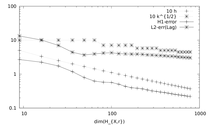
Figure 1: Errors for $r=0.2$ and $\tau=1.5$.

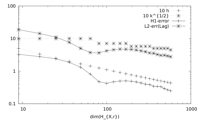
Figure 2: Errors for $r=0.2$ and $\tau=2.5$.

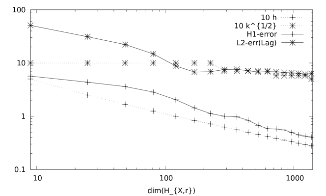
Figure 3: Errors for $r=0.1$ and $\tau=1.5$.

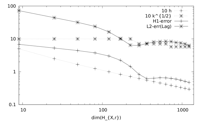
Figure 4: Errors for $r=0.1$ and $\tau=2.5$.

References

[1]
I. Babuška.
The finite element method with Lagrangian multipliers.
Numer. Math., 20 (1972/73), 179–192.
[2]
J. Bergh and J. Löfström.
Interpolation Spaces: An Introduction.
Springer-Verlag, Berlin, 1976.
[3]
S. C. Brenner and L. R. Scott.
The Mathematical Theory of Finite Element Methods.
Springer, Berlin, 2002.
[4]
Y. Duan and Y.-J. Tan.
A meshless Galerkin method for Dirichlet problems using radial
basis functions.
J. Comput. Appl. Math., 196 (2006), 394–401.
[5]
G. N. Gatica, M. Healey, and N. Heuer.
The boundary element method with Lagrangian multipliers.
Numer. Methods Partial Differential Equations, 25
(2009), 1303–1319.
[6]
P. Grisvard.
Elliptic Problems in Nonsmooth Domains.
Pitman, Boston, 1985.
[7]
N. Heuer and T. Tran.