Magnetic flux loop in high-energy heavy-ion collisions

Abstract

We consider the expectation value of a chromo-magnetic flux loop in the immediate forward light cone of collisions of heavy nuclei at high energies. Such collisions are characterized by a non-linear scale $Q_{s}$ where color fields become strong. We find that loops of area greater than $\sim 1.5/Q_{s}^{2}$ exhibit area law behavior, which determines the scale of elementary flux excitations (“vortices”). We also estimate the magnetic string tension, $\sigma_{M}\simeq 0.12\,Q_{s}^{2}$. By the time $t\sim 1/Q_{s}$ even small loops satisfy area law scaling. We describe corrections to the propagator of semi-hard particles at very early times in the background of fluctuating magnetic fields.

Collisions of heavy ions at high energies provide opportunity to study non-linear dynamics of strong QCD color fields Mueller:1999wm . The field of a very dense system of color charges at rapidities far from the source is determined by the classical Yang-Mills equations with a recoilless current along the light cone MV . It consists of gluons characterized by a transverse momentum $p_{T}$ on the order of the density of valence charges per unit transverse area $Q_{s}^{2}$ JalilianMarian:1996xn ; this saturation momentum scale separates the regime of non-linear color field interactions at $p_{T}\,\,\vbox{\hbox{$\buildrel\displaystyle<\over{\sim}$}}\,\,Q_{s}$ or distances $r\,\,\vbox{\hbox{$\buildrel\displaystyle>\over{\sim}$}}\,\,1/Q_{s}$ from the perturbative regime at $p_{T}\gg Q_{s}$. Near the center of a large nucleus this scale is expected to exceed $\sim 1.5$ GeV at BNL-RHIC or CERN-LHC collider energies, for a probe in the adjoint representation of the color gauge group. The classical field solution provides the leading contribution to an expansion in terms of the coupling and of the inverse saturation momentum.

The soft field produced in a collision of two nuclei is then a solution of the Yang-Mills equations satisfying appropriate matching conditions on the light cone Kovner:1995ja . Most interestingly, right after the impact strong longitudinal chromo-magnetic fields $B_{z}\sim 1/g$ develop due to the fact that the individual projectile and target fields do not commute Fries:2006pv ; TL_LM . They fluctuate according to the random local color charge densities of the valence sources. In this Letter we show that magnetic loops $W_{M}$ exhibit area law behavior, and we compute the magnetic string tension. Furthermore, we argue that at length scales $\sim 1/Q_{s}$ the field configurations might be viewed as uncorrelated Z(N) vortices. At finite times $\sim 1/Q_{s}$ after the collision area law behavior is observed even for rather small Wilson loops. Finally, we sketch how the background of magnetic fields affects propagation of semi-hard particles with transverse momenta somewhat above $Q_{s}$.

Consider a spatial Wilson loop with radius $R$ in the plane transverse to the beams,

$$M(R) = {\cal P}\exp\left(ig\int\limits_{-\pi}^{\pi}d\theta\;\frac{\partial x^{i}}{\partial\theta}A^{i}\right)$$

$$W_{M}(R) = \frac{1}{N_{c}}\left<{\rm tr}\,M(R)\right>~{},$$ (1)

where $x=R(\cos\theta,\sin\theta)$, and path ordering is with respect to the angle $\theta$; in numerical lattice simulations it is more convenient to employ a square loop. We compare, also, to the expectation value of the Z($N_{c}$) part of the loop; for a magnetic field configuration corresponding simply to a superposition of independent vortices the loop should equal $\exp(2\pi i\,n/N_{c})$, with $n$ the total vortex charge piercing the loop. Thus, for two colors we compute

$$W_{M}^{Z(2)}(R)=\left<\mathop{\mathrm{sgn}}{\rm tr}\,M(R)\right>$$ (2)

where $\mathop{\mathrm{sgn}}()$ denotes the sign function. Comparing (1) to (2) tests the interpretation that the drop-off of $W_{M}(R)$ is due to Z($N_{c}$) vortices, without requiring gauge fixing of the SU($N_{c}$) links Stack:2000he .

The field in the forward light cone immediately after a collision Kovner:1995ja , at proper time $\tau\equiv\sqrt{t^{2}-z^{2}}\to 0$, is given in light cone gauge by $A^{i}=\alpha_{1}^{i}+\alpha_{2}^{i}$. In turn, before the collision the individual fields of projectile and target are 2d pure gauges,

$$\alpha^{i}_{m}=\frac{i}{g}\,U_{m}\,\partial^{i}U_{m}^{\dagger}~{}~{}~{}~{},~{}~{}~{}~{}\partial^{i}\alpha^{i}_{m}=g\rho_{m}~{},$$ (3)

where $m=1,\,2$ labels projectile and target, respectively, and $U_{m}$ are SU(N) gauge fields.

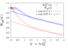
Figure 1: Expectation value of the magnetic flux loop right after a collision of two nuclei (time $\tau=+0$) as a function of its area $A^{\prime}\equiv A\,Q_{s}^{2}$. We define $Q_{s}^{2}=(C_{F}/2\pi)\,g^{4}\mu^{2}$. Symbols show numerical results for $SU(2)$ Yang-Mills on a $4096^{2}$ lattice; the lattice spacing is set by $g^{2}\mu_{L}=0.0661$. The solid and dashed lines represent fits over the range $4\geq A^{\prime}\geq 2$. The short dotted line shows $\cos 2A^{\prime}$ for $A^{\prime}<0.3$.

Eqs. (3) can be solved either analytically in an expansion in the field strength Kovner:1995ja or numerically on a lattice CYMlatt .

The large-$x$ valence charge density $\rho$ is a random variable. For a large nucleus, the effective action describing color charge fluctuations is quadratic,

$$S_{\rm eff}[\rho^{a}]=\frac{\rho^{a}({\bf x})\rho^{a}({\bf x})}{2\mu^{2}}~{}~{}~{},~{}~{}~{}\langle\rho^{a}({\bf x})\,\rho^{b}({\bf y})\rangle=\mu^{2}\delta^{ab}\delta({\bf x}-{\bf y})~{},$$ (4)

with $\mu^{2}$ proportional to the thickness of a given nucleus MV . The variance of color charge fluctuations determines the saturation scale $Q_{s}^{2}\sim g^{4}\mu^{2}$ JalilianMarian:1996xn . The coarse-grained effective action (4) applies to (transverse) area elements containing a large number of large-$x$ “valence” charges, $\Delta A_{\perp}\,\mu^{2}\sim\Delta A_{\perp}\,Q_{s}^{2}/g^{4}\gg 1$. The densities $\rho^{a}({\bf x})$ at two different points are independent so that their correlation length within the effective theory is zero. However, this is not so for the gauge fields $A^{i}$ which do exhibit a finite screening length m_screen .

In fig. 1 we show numerical results for $W_{M}$ immediately after a collision. It exhibits area law behavior for loops larger than $A\,\,\vbox{\hbox{$\buildrel\displaystyle>\over{\sim}$}}\,\,2/Q_{s}^{2}$. The corresponding “magnetic string tension” is $\sigma_{M}/Q_{s}^{2}=0.12(1)$. The area law indicates uncorrelated magnetic flux fluctuations through the Wilson loop and that the area of magnetic vortices is rather small, their radius being on the order of $R_{\rm vtx}\sim 0.8/Q_{s}$. We do not observe a breakdown of the area law up to $A\sim 4/Q_{s}^{2}$, implying that vortex correlations are small at such distance scales. Also, restricting to the Z(2) part reduces the magnetic flux through small loops but $\sigma_{M}$ is comparable to the full SU(2) result, if somewhat smaller.

The numerically small vortex size that we find is parametrically consistent with the classical Gaussian approximation at weak coupling which, as already mentioned above, applies for areas $\Delta A_{\perp}\gg g^{4}/Q_{s}^{2}$. Corrections to $S_{\rm eff}$ of higher order in $\rho$ Srho as well as due to quantum fluctuations Berges:2012cj of the fields should be investigated in the future.

Since the field $\alpha^{i}_{m}$ of a single nucleus is a pure gauge it follows that $W_{M}^{\rm sngl}(\alpha_{m}^{i})=1$. However, beyond linear order the field in the forward light cone, $A^{i}=\alpha^{i}_{1}+\alpha^{i}_{2}$ is not a pure gauge and so $W_{M}(A^{i})\neq 1$. As discussed in the appendix, for small loops the correction

$$W_{M}(\alpha_{1}^{i}+\alpha_{2}^{i})-1\sim-A^{2}$$ (5)

is proportional to the square of the area of the loop. There is no contribution at order $\sim A$, hence no area law behavior and no vortices, even though there is, of course, a non-zero longitudinal magnetic field even at the “naive” perturbative level:

$$\frac{g^{2}}{N_{c}}\langle{\rm tr}\,B_{z}({\bf r})\,B_{z}({\bf r^{\prime}})\rangle=4\frac{N_{c}^{2}}{N_{c}^{2}-1}\,Q_{s1}^{2}Q_{s2}^{2}\log^{2}\frac{1}{|{\bf r}-{\bf r^{\prime}}|\,\Lambda}~{}.$$ (6)

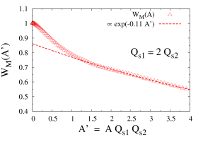
Figure 2: Same as fig. 1 for asymmetric projectile and target saturation momenta.

Eq. (5) applies for small $AQ_{s}^{2}\ll 1$ while the non-perturbative lattice result exhibits area law behavior at $\tau=+0$ for $AQ_{s}^{2}\,\,\vbox{\hbox{$\buildrel\displaystyle>\over{\sim}$}}\,\,1$. It indicates the presence of resummed screening corrections for magnetic fields m_screen . To see this more explicitly it is useful to notice that $\sigma_{M}\sim Q_{s}^{2}$ is in fact $\sigma_{M}\sim Q_{s1}Q_{s2}$, proportional to the product of single powers of the respective saturation scales of projectile and target. We have verified this numerically in fig. 2. Naive perturbation theory can only produce even powers of the two-point function $\sim Q_{s}^{2}$.

To estimate the density of vortices one can consider a simple combinatorial model whereby the area $A$ of the loop is covered by patches of size $1/Q_{s}^{2}$ containing a Z(2) vortex with probability $p$. Averaging over random, uncorrelated vortex fluctuations leads to preskill

$$W_{M}(A)\sim\exp\left(-\frac{\pi^{2}}{4}\;p(1-p)AQ_{s}^{2}\right)~{},$$ (7)

or $\sigma_{M}=(\pi^{2}/4)\;p(1-p)Q_{s}^{2}$. From this relation we estimate that the probability of finding a vortex within an area $1/Q_{s}^{2}$ is $p\simeq 1/20$.

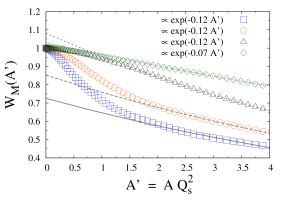
Figure 3: Time evolution of the magnetic flux loop after a collision of two nuclei ($4096^{2}$ lattice, $g^{2}\mu_{L}=0.05$). From bottom to top, the curves correspond to time $\tau\times g^{2}\mu=0$, 1, 2, 3, where $g^{2}\mu\simeq 3Q_{s}$ so that $\tau=3/(g^{2}\mu)$ corresponds to about $\tau\simeq 1/Q_{s}$ in physical units.

In fig. 3 we show the time evolution of the magnetic flux loop after a collision. The magnetic field strength decreases due to longitudinal expansion and so $W_{M}$ approaches unity. On the other hand, the onset of area law behavior is pushed to smaller loops, implying that the size of elementary flux excitations or “vortices” decreases; by the time $\tau\sim 1/Q_{s}$ area law behavior is satisfied even for rather small loops. Since long wavelength magnetic fields remain even at times $\sim 1/Q_{s}$, it will be important in the future to understand the transition of $W_{M}$ to behavior expected in thermal QCD where $\sigma_{M}\sim(g^{2}T)^{2}$ kajantie . In the context of late-time behavior much beyond $t\sim 1/Q_{s}$ we refer to ref. Berges where area law scaling of spatial loops has been observed for classical field configurations emerging from unstable plasma evolution.

We have also investigated the dependence of the magnetic flux loop in the adjoint representation on its area,

$$W_{M}^{\rm adj}=\frac{1}{N_{c}^{2}-1}\left<|{\rm tr}\,M|^{2}-1\right>~{},$$ (8)

and found behavior similar to fig. 3. The adjoint magnetic string tension is about two times larger, as expected from (8).

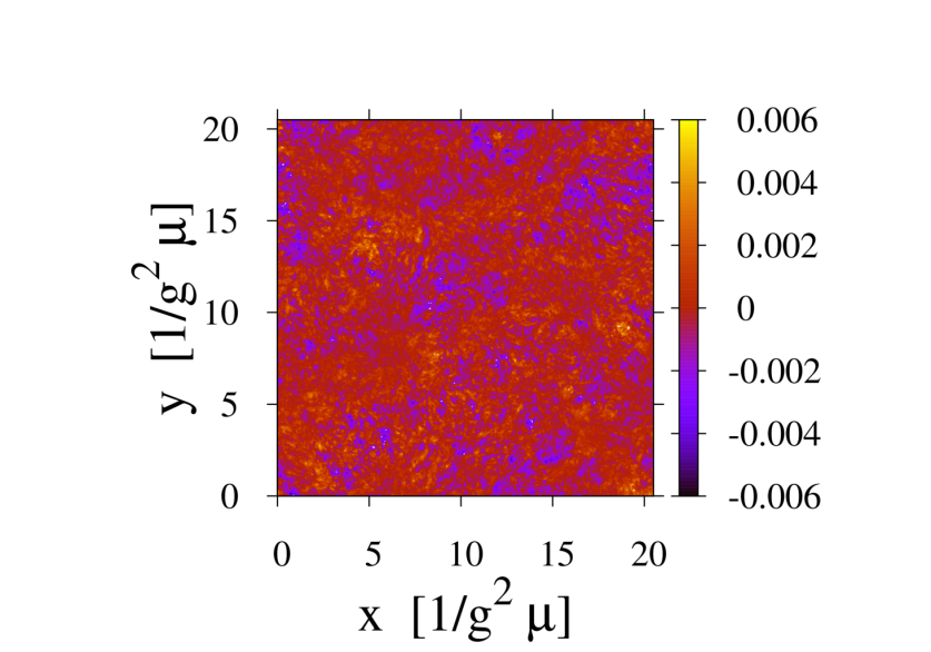
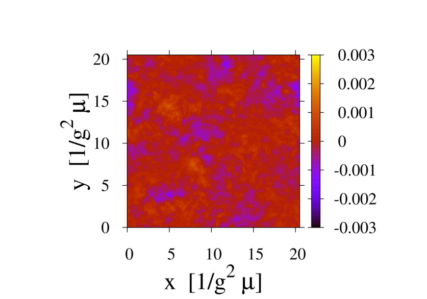
Figure 4: Color-3 component of the magnetic field $F_{xy}^{3}(x,y)$ in the transverse plane at time $\tau=+0$ (top) and $1/g^{2}\mu\sim 1/3Q_{s}$ (bottom) for a single configuration of color charge sources $\rho$.

The third color component of the longitudinal magnetic field is shown in fig. 4, using a random residual gauge for $A^{i}$. Domain-like structures where the magnetic field is either positive or negative are clearly visible; they lead to the above-mentioned area law of the Wilson loop. Also, one can see that in time the magnetic fields become weaker and smoother.

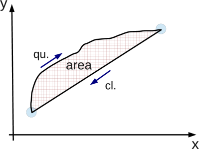
Figure 5: Area enclosed by a quantum mechanical path shifted by about one de Broglie wavelength from the extremal classical path.

Thus far we have not addressed the longitudinal structure of the initial fields. Our solution of eqs. (3) is boost invariant and so, naively, the two-dimensional vortex structures mentioned above would form boost invariant strings. However, this simple picture could be modified by longitudinal smearing of the valence charge distributions Fukushima:2007ki and therefore requires more detailed consideration.

The magnetic fields modify the propagation of semi-hard modes with $p_{T}$ not too far above $Q_{s}$. Quantum mechanically, the transition amplitude from a state $\left|x_{i},t_{i}\right>$ to $\left|x_{f},t_{f}\right>$ is given by a Feynman sum over paths,

$$\int_{0}^{\infty}ds\int{\cal D}x^{\mu}\left<\exp\,i\int\limits_{0}^{s}d\tau\left(m\dot{x}^{2}+gA_{\mu}\dot{x}^{\mu}\right)\right>\sim$$

$$\int_{0}^{\infty}ds\int{\cal D}x^{\mu}\exp\,\left(i\int\limits_{0}^{s}d\tau\,m\dot{x}^{2}\right)\;\exp(-\sigma_{M}A)~{},$$ (9)

where $x^{\mu}(\tau)$ is a parametrization of the path with the given boundary conditions and length $s$; and $\dot{x}^{\mu}=dx^{\mu}/d\tau$. Here, the area $A$ is that enclosed by a quantum mechanical path from the initial to the final point returning to ${\bf x}_{i}$ via the classical path; see fig. 5. The classical path is obtained by extremizing the action but a single path is a set of measure zero. Semi-classical paths can dominate the integral only if there is constructive interference among neighboring paths from within a de Broglie distance. On the other hand, destructive interference of such paths leads to Anderson localization of the wave function.

Hence, up to a numerical factor, the area in eq. (9) should be given by $A\sim s/p_{T}$. Integrating over the Schwinger parameter then leads to the propagator

$$\frac{i}{p^{2}+i\sigma_{M}\frac{m}{p_{T}}}~{},$$ (10)

where $\sigma_{M}=0.12\,Q_{s}^{2}$ from above and $m$ is the mass (time-like virtuality) of the particle. This expression accounts for corrections to free propagation and could be useful for studies of the dynamics of the very early stage of a heavy-ion collision.

We obtain a rather interesting picture of the very early stage of ultrarelativistic heavy-ion collisions. Magnetic Wilson loops of area $\,\,\vbox{\hbox{$\buildrel\displaystyle>\over{\sim}$}}\,\,2/Q_{s}^{2}$ effectively exhibit area law behavior which implies uncorrelated magnetic Z(N) vortex-like flux beyond the scale $R_{\rm vtx}\sim 0.8/Q_{s}$. We do expect that corrections to this picture appear at much larger distance scales and we intend to study these in detail in the future. The vortex structure of the longitudinal magnetic field modifies propagation of particle-like modes with de Broglie wavelength somewhat larger than $Q_{s}$.

Appendix A Appendix: Perturbative limit of the magnetic Wilson loop at $\tau=0$

In this appendix we outline the “naive” perturbative expansion of the loop with the Gaussian contractions. We stress that since magnetic fields at $\tau=0$ are screened over distances $\sim 1/(5Q_{s})$ m_screen , that this naive expansion can not be applied in the regime of interest in the present paper.

To determine $W_{M}(A^{i})$ we need to determine the “correction” in $A^{i}=\alpha_{1}^{i}+\alpha_{2}^{i}$ from a pure gauge. From the Baker-Campbell-Hausdorff relation,

$$W_{M}(A^{i})\simeq\frac{1}{N_{c}}{\rm tr}\,\exp\left(-\frac{1}{2}[X_{1},X_{2}]\right)~{},$$ (11)

where terms of third order in the fields have been dropped from the exponent; and $X_{m}$ is $\alpha_{m}^{i}$ integrated along the loop.

In the weak field limit Kovner:1995ja

$$\alpha_{m}^{i}=-\partial^{i}\Phi_{m}+\frac{ig}{2}\left(\delta^{ij}-\partial^{i}\frac{1}{\nabla_{\perp}^{2}}\partial^{j}\right)\left[\Phi_{m},\partial^{j}\Phi_{m}\right]+\cdots$$ (12)

The first term on the rhs of eq. (12) does not contribute to the integral of $\alpha_{m}^{i}$ over a closed loop.

We can express the square of the exponent on the r.h.s. of (11) as

$$h^{2}\equiv\frac{1}{16}f^{abc}f^{dec}X_{1}^{a}X_{1}^{d}X_{2}^{b}X_{2}^{e}~{},$$ (13)

so that for two colors

$$W_{M}(A^{i})\simeq\left<\cos h\right>_{\rho_{1},\rho_{2}}\simeq 1-\frac{1}{2}\langle h^{2}\rangle~{}.$$ (14)

Eq. (13) contains four integrations over the periphery of the loop, two of which will be removed by the $\langle\cdot\rangle_{\rho_{1}}$ and $\langle\cdot\rangle_{\rho_{2}}$ contractions; c.f. eq. (4). Hence $\langle h^{2}\rangle\sim A^{2}\mu^{4}$ is proportional to the square of the area of the loop. Fig. 1 shows that by matching to the lattice data at $A^{\prime}\ll 1$ we estimate $h\approx 2A^{\prime}$.

References

- (1) A. H. Mueller, Nucl. Phys. B 558, 285 (1999).
- (2) L. D. McLerran and R. Venugopalan, Phys. Rev. D 49, 2233 (1994), Phys. Rev. D 49, 3352 (1994); Y. V. Kovchegov, Phys. Rev. D 54, 5463 (1996).
- (3) J. Jalilian-Marian, A. Kovner, L. D. McLerran and H. Weigert, Phys. Rev. D 55, 5414 (1997).
- (4) A. Kovner, L. D. McLerran and H. Weigert, Phys. Rev. D 52, 6231 (1995); Phys. Rev. D 52, 3809 (1995).
- (5) R. J. Fries, J. I. Kapusta and Y. Li, nucl-th/0604054.
- (6) T. Lappi and L. McLerran, Nucl. Phys. A 772, 200 (2006).
- (7) J. D. Stack, W. W. Tucker and A. Hart, hep-lat/0011057.
- (8) A. Krasnitz, Y. Nara and R. Venugopalan, Phys. Rev. Lett. 87, 192302 (2001); T. Lappi, Phys. Rev. C 67, 054903 (2003); Eur. Phys. J. C 55, 285 (2008).
- (9) A. Dumitru, H. Fujii and Y. Nara, arXiv:1305.2780 [hep-ph].
- (10) A. Dumitru and E. Petreska, Nucl. Phys. A 879, 59 (2012); A. Dumitru, J. Jalilian-Marian and E. Petreska, Phys. Rev. D 84, 014018 (2011).
- (11) J. Berges and S. Schlichting, arXiv:1209.0817 [hep-ph].
-
(12)
see, for example, J. Preskill, “Lecture Notes on Quantum Field
Theory”,
http://www.theory.caltech.edu/~preskill/notes.html - (13) T. Appelquist and R. D. Pisarski, Phys. Rev. D 23, 2305 (1981); E. Manousakis and J. Polonyi, Phys. Rev. Lett. 58, 847 (1987); G. S. Bali, J. Fingberg, U. M. Heller, F. Karsch and K. Schilling, Phys. Rev. Lett. 71, 3059 (1993); J. Alanen, K. Kajantie and V. Suur-Uski, Phys. Rev. D 80, 075017 (2009).
- (14) J. Berges, S. Scheffler and D. Sexty, Phys. Rev. D 77, 034504 (2008).
- (15) K. Fukushima, Phys. Rev. D 77, 074005 (2008).