The pulsar spectral index distribution

Abstract

The flux density spectra of radio pulsars are known to be steep and, to first order, described by a power-law relationship of the form $S_{\nu}\propto\nu^{\alpha}$, where $S_{\nu}$ is the flux density at some frequency $\nu$ and $\alpha$ is the spectral index. Although measurements of $\alpha$ have been made over the years for several hundred pulsars, a study of the intrinsic distribution of pulsar spectra has not been carried out. From the result of pulsar surveys carried out at three different radio frequencies, we use population synthesis techniques and a likelihood analysis to deduce what underlying spectral index distribution is required to replicate the results of these surveys. We find that in general the results of the surveys can be modelled by a Gaussian distribution of spectral indices with a mean of –1.4 and unit standard deviation. We also consider the impact of the so-called “Gigahertz-peaked spectrum” pulsars proposed by Kijak et al. The fraction of peaked spectrum sources in the population with any significant turn-over at low frequencies appears to be at most 10%. We demonstrate that high-frequency ($>2$ GHz) surveys preferentially select flatter-spectrum pulsars and the converse is true for lower-frequency ($<1$ GHz) surveys. This implies that any correlations between $\alpha$ and other pulsar parameters (for example age or magnetic field) need to carefully account for selection biases in pulsar surveys. We also expect that many known pulsars which have been detected at high frequencies will have shallow, or positive, spectral indices. The majority of pulsars do not have recorded flux density measurements over a wide frequency range, making it impossible to constrain their spectral shapes. We also suggest that such measurements would allow an improved description of any populations of pulsars with ‘non-standard’ spectra. Further refinements to this picture will soon be possible from the results of surveys with the Green Bank Telescope and LOFAR.

1 Introduction

Radio pulsars are known to have steep flux-density spectra (e.g. Sieber, 1973) which approximately follow the power-law relationship

$$S_{\nu}\propto\nu^{\alpha}$$ (1)

for observed flux density $S_{\nu}$ at frequencies $\nu>100~{}\mathrm{MHz}$ where $\alpha$ is the spectral index. Although a number of multi-frequency flux measurements of pulsars were carried out over the years (Sieber, 1973; Backer & Fisher, 1974; Malofeev & Malov, 1980; Slee et al., 1986), the first systematic study of the spectral indices for a large number of pulsars was carried out by Lorimer et al. (1995) who published spectra on 280 pulsars based on flux density measurements carried out for up to five different radio frequencies between 0.4 and 1.6 GHz using the Lovell radio telescope. The resulting analysis showed that the average spectral index for the observationally selected pulsar sample was $\alpha=-1.6\pm 0.3$. More recent work by Maron et al. (2000) derived a mean value of $\alpha=-1.8\pm 0.2$, where the range of frequencies was extended, in many cases, up to 5 GHz. Maron et al. (2000) also found evidence for $\sim 10\%$ of pulsars in their sample being best fit using a double power law, described by parameters $\alpha_{1}$ at lower frequencies and $\alpha_{2}$ at higher frequencies. Typically $\alpha_{2}$ is steeper, $|\alpha_{2}|>|\alpha_{1}|$, with the spectral break at a frequency of $\sim 1\mathrm{GHz}$.

Table 1: Observational parameters for the three pulsar surveys discussed in the text: the Parkes southern pulsar survey (PKS70, Manchester et al., 1996), the Parkes multi-beam pulsar survey (PMPS, Manchester et al., 2001) and the Parkes 6.5 GHz multi-beam pulsar survey (MMB, Bates et al., 2011).

	PKS70	PMPS	MMB
Number of beams	1	13	7
Polarizations/beam	2	2	2
Centre frequency (MHz)	436	1352	6591
Frequency channels	256	96	192
Channel width (MHz)	0.125	3	3
Gain ($\mathrm{KJy}^{-1}$)	0.64	$\sim 0.7$	0.6
Integration time (s)	157.3	2100	1055
Sampling interval ($\mu$s)	300	250	125
Region covered	$\delta<0\degree$	$100\degree\leq l\leq 50\degree$	$-60\degree\leq l\leq 30\degree$
		$|b|\leq 5\degree$	$|b|\leq 0.25\degree$
Pulsars detected ($P>50~{}\mathrm{ms}$)	279	1038	18

An interesting additional effect noticed by Maron et al. was the high-frequency spectral turnovers observed for PSRs B1823–13 and B1838–04. While turnovers are frequently observed at frequencies below $\sim 100$ MHz (e.g. Izvekova et al., 1981), the presence of such turnovers at frequencies around 1 GHz seems to be unusual. Recent research on a subset of these pulsars (not including PSR B1838–04) with so-called gigahertz-peaked spectra (hereafter GPS; see Kijak et al., 2011a, b) indicates that these sources can be fitted by

$$S_{\nu}=10^{ax^{2}+bx+c};\quad x=\log_{10}\nu,$$ (2)

an extension of Equation 1, where $b$ is equivalent to $\alpha$ in the case where $a=0$. Kijak et al. (2011a) list five known GPS pulsars, with measured values of the turnover parameter, $a$, ranging from $-7.3$ to $-1.2$. However, both they and, more recently, Dembska et al. (2012) observe that PSR B1259$-$63 displays many different spectral types depending upon the orbital phase when flux measurements are taken — including a GPS-type spectrum when near periastron. They conclude that non-standard spectral shapes in the pulsar population could be linked to unusual environments around pulsars.

While the observed distribution of pulsar spectra has been the subject of much investigation (Lorimer et al., 1995; Maron et al., 2000), the underlying distribution for the population is currently not understood. Knowledge of this distribution has important implications for the pulsar emission mechanism, and for derivation of the pulsar luminosity function over a broad range of radio frequencies. The latter point has been largely overlooked so far, with population analyses (e.g. Lorimer et al., 2006; Faucher-Giguère & Kaspi, 2006) choosing to focus on the hugely successful 20-cm Multibeam Pulsar Surveys carried out at Parkes (for a review, see Lyne, 2008). The advantage of this approach is that it does not require any knowledge of the radio spectrum to constrain the population of sources visible at 20-cm. The disadvantage is that it precludes any reliable statements being made about the population of pulsars visible at other observing frequencies.

In this paper, we aim to use detailed Monte Carlo simulations of pulsar surveys carried out at multiple frequencies to constrain the underlying distribution of $\alpha$ in the pulsar population. The focus of this work is on the normal (i.e. non-recycled) population. Although millisecond pulsar spectra appear to be similar to normal pulsars (see, e.g., Kramer et al. 1998), a detailed study of this population will be deferred to a future paper. In § 2 we review the surveys which define our sample. In § 3 we describe the relevant population modelling techniques used in this study. In § 4 we use our sample to place constraints on the underlying spectral index distribution assuming it to be a simple power-law, and discuss how our results would change were the surveys found to be incomplete. In § 5 we investigate what fraction of the population could display alternative spectral shapes. Finally, the implications of our results are discussed in § 6.

Table 2: Parameters used to simulate the pulsar population in §4.1.

Radial distribution model	Lorimer et al. (2006)
Galactic latitude scale height	330 pc
Luminosity distribution	Log-normal
$\langle{\log\,\mathrm{L~{}(mJy~{}kpc^{2})}}\rangle$	$-1.1$
$\mathrm{std}(\log\,\mathrm{L~{}(mJy~{}kpc^{2})}))$	$0.9$
Period distribution	Log-normal
$\langle{\log\,\mathrm{P~{}(ms)}}\rangle$	$2.7$
$\mathrm{std}(\log\,\mathrm{P~{}(ms)})$	$-0.34$
Scattering model	Bhat et al. (2004)
Number of detectable pulsars	1038
in the PMPS survey

2 Pulsar surveys

Many surveys of the Galactic plane for pulsars have been performed, at different radio frequencies, despite the steep spectral behaviour discussed in the previous section. This is because of two effects which limit sensitivity at low observing frequencies. Firstly synchrotron radiation from free electrons in the Galactic magnetic field causes the sky background temperature, $T_{\mathrm{sky}}$, to vary with frequency as $\nu^{-2.6}$ (Lawson et al., 1987). At low frequencies, the sky temperature can then dominate the system temperature and reduce sensitivity to pulsars. Secondly, as signals from pulsars traverse the interstellar medium, they are scattered, which causes them to be broadened by a timescale which scales approximately as $\nu^{-3.5}$ for high-DM pulsars (Löhmer et al., 2001; Bhat et al., 2004). Since this effect is not easily removed, low-frequency surveys are severely hampered when searching for faint pulsars in the Galactic plane. As a result of these issues, pulsar surveys have to compromise between these two effects, and the reduced flux density which is observed from pulsars at higher frequencies. Three examples of pulsar surveys at three observing frequencies are outlined below. Table 1 summarises each of these surveys.

By far the most successful pulsar survey to date was the Parkes multi-beam pulsar survey (hereafter the PMPS survey, Manchester et al., 2001) which, to date, has discovered close to 800 pulsars, essentially doubling the number previously known. The PMPS observed a thin strip of the Galactic plane, Galactic latitude $|b|<5\degree$, Galactic longitude $100\degree<l<50\degree$, at a frequency of 1.4 GHz using the 64-metre Parkes radio telescope. The Parkes southern pulsar survey (PKS70, Manchester et al., 1996) was a survey of the entire southern sky, $\delta<0\degree$, at a frequency of 436 MHz. The survey discovered 101 pulsars, many of which were at high Galactic latitudes. The Parkes 6.5 GHz multi-beam pulsar survey (MMB, Bates et al., 2011) used the seven-beam Parkes Methanol Multi-beam receiver to survey the Galactic plane in the region $-60\degree\leq l\leq 30\degree,|b|\leq 0.25\degree$ at a frequency of 6.5 GHz. This survey was specifically designed to discover pulsars deep in the Galactic plane which would otherwise be obscured by the interstellar scattering discussed above. This survey discovered two pulsars, indicating that there are few pulsars in the direction of the Galactic centre whose spectra obey a shallow or flat power law.

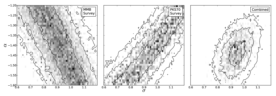
Figure 1: Grey scale plots of the likelihood, ${\cal L}$ (as defined in § 4.2) as a function of the mean, $\alpha$, and standard deviation , $\sigma$, of the input spectral index distribution. The left and centre plots show the results for the MMB and PKS70 surveys respectively, and the right-hand plot is the product of the likelihoods in each bin. Significance contours of 1, 2 and 3 standard deviations — calculated by Equation 3 — are overlaid. The total confidence levels in the right-hand panel were calculated by summing the MMB and PKS70 survey confidence levels in quadrature.

3 Population synthesis

There are two main techniques which are commonly applied when simulating the pulsar population (for a recent review, see Lorimer, 2011). The first is the “snapshot” approach, which is to synthesise a pulsar population in the current epoch based entirely upon the known statistics of the observed population (see, e.g., Lorimer et al., 2006). The second is a more computationally-involved, fully dynamical technique, where a model galaxy of pulsars is given initial birth positions and parameters, then allowed to evolve using models of the pulsar spin-down and Galactic potential (see, e.g., Faucher-Giguère & Kaspi, 2006; Ridley & Lorimer, 2010). The model population can be compared to the results of previous pulsar surveys to check its validity.

In this work, where the main focus is to explore the dependence of pulsar spectra on survey yields, we will use the snapshot approach which will make no assumptions about the birth parameters of pulsars, or their subsequent evolution. Instead we are able to produce model populations using parameters obtained purely from observations — though it must be remembered that this technique is still reliant on some models, for example the Galactic electron distribution, for which no one model entirely describes the observed data. Following standard practice, we adopt the model of Cordes & Lazio (2002) in our simulations described below.

4 Obtaining the spectral index distribution of normal pulsars

4.1 Method

For all our model populations, we adopted the parameters given in Table 2, and used the psrpop software package (based upon work done for Lorimer et al., 2006) to generate synthetic pulsar populations which we grew in size until we obtained a sample of 1038 model pulsars detected by the PMPS survey. The number of detections in the MMB and PKS70 surveys was not constrained. The parameters were chosen to match the studies of Lorimer et al. (2006) and Faucher-Giguère & Kaspi (2006), who found that a log-normal luminosity distribution accurately describes the known population. To simulate the spectral properties of pulsars, we initially adopted a simple approach and assumed that the pulsar spectral indices are normally distributed (as in Lorimer et al., 1995; Maron et al., 2000). Subsequent modifications to this technique are described in §5.1 and 5.2. For this simple model, we allowed the mean spectral index, $\alpha$, and standard deviation, $\sigma$, of this distribution to vary in the range $-2.0<\alpha<-1.0$ and $0.0<\sigma<2.0$ (each in steps of 0.01). Each combination of $\alpha$ and $\sigma$ was realised 500 times using different starting seeds for the random number generators. The resulting set of 500 model populations were analysed as described below.

4.2 Analysis

We selected the sample of observed pulsars based on the results of the PKS70, PMPS and MMB surveys with which we could compare the simulations. From the ATNF Pulsar Catalogue (Manchester et al., 2005), there are a total of 1197 pulsars with periods $P>50~{}\mathrm{ms}$ detected in one or both of the PKS70 and PMPS surveys. From Bates et al. (2011), 18 pulsars were observed in the MMB survey, four of which were not observed in the PKS70 or PMPS surveys. This gives a total of 1201 pulsars which have been observed in one or more of the surveys; Table 1 gives a breakdown of the number of pulsars by survey. The aforementioned period cut-off effectively removes the recycled pulsars from this sample and none of the pulsars in the list of 1201 is associated with any known globular cluster.

The psrpop program survey was used on each of the model populations to create a list of detected pulsars for the surveys. To measure the effectiveness of our models at reproducing the observed survey yields, we adopted the following simple likelihood analysis. For each bin in the $\alpha$-$\sigma$ space, two likelihood values, ${\cal L}_{\rm MMB}$ and ${\cal L}_{\rm PKS70}$, were computed. These likelihoods are defined to be the fraction of 500 realisations for which the simulated survey detected the same number of pulsars as in the catalogue, for both the MMB and PKS70 surveys. When presenting our results below, we show the individual likelihoods, and their product ${\cal L}={\cal L}_{\rm MMB}\times{\cal L}_{\rm PKS70}$. The maximum value of ${\cal L}$ allows us to constrain the ranges of $\alpha$ and $\sigma$ which best match the observed survey yields.

Confidence levels, $\cal C$, were also independently calculated in each $\alpha$-$\sigma$ bin,

$${\cal C}=\frac{\bar{n}_{\mathrm{sim}}-n_{\mathrm{cat}}}{\mathrm{stddev}(n_{\mathrm{sim}})}$$ (3)

where $\bar{n}_{\mathrm{sim}}$ is the mean number of pulsars detected in each realisation, $n_{\mathrm{cat}}$ is the number of pulsars detected in the survey, according to the pulsar catalogue, and $\mathrm{stddev}(n_{\mathrm{sim}})$ is the standard deviation of $n_{\mathrm{sim}}$ across the 500 realisations.

4.3 Results

The results of the analysis procedure which gives the likelihoods, ${\cal L}_{\rm MMB}$ and ${\cal L}_{\rm PKS70}$, for the MMB and PKS70 surveys are shown in Figure 1. Note that the region of high likelihood in the $\alpha$-$\sigma$ plane is oriented in a reasonable way; the MMB survey only allows steep values of $\alpha$ if there is a large width in the distribution, whereas the PKS70 survey only allows shallow $\alpha$ values if the distribution is wide. The product of those results, ${\cal L}$, is also shown in the right-hand panel, which gives the overall result shown in Figure 2, where the likelihoods have been summed in the $\alpha$ and $\sigma$ directions to produce marginalized probability density functions. Fitting a gaussian to these distributions provides a very straightforward way to quantify them. From these fits, we find the optimum spectral index distribution to be $\bar{\alpha}=-1.41\pm 0.06$ and $\bar{\sigma}=0.96\pm 0.05$. To illustrate how the models fit the data in the catalogue, Figure 3 shows average spectral index histograms for a further 100 realisations performed with the values of $\bar{\alpha}$ and $\bar{\sigma}$ obtained above.

In the early stages of this work, we had initially hoped to use the observed spectral index distributions obtained from the pulsar catalogue (the majority of these values are taken from Lorimer et al. (1995)) as part of the analysis, however, the completeness of these samples was found to be too low to produce reliable results. Only 4/18 pulsars in the MMB survey have measured spectral indices, 84/279 pulsars in the PKS70 survey, and 83/1038 pulsars in the PMPS survey. As the catalogue values of $\alpha$ are so incomplete, Fig. 3 serves as something of a prediction for further measurements of the spectral indices of pulsars detected in the MMB and PKS70 surveys — there are a dearth of pulsars which so far have had their spectral indices measured to be $\alpha<-2.0$ or $\alpha>0.0$. Further observational work in this area would be extremely valuable in refining this model, and our subsequent modifications to it discussed below.

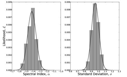
Figure 2: Marginalized probability density functions obtained for each spectral index (left) and standard deviation (right) bin used in our simulations. Best fits are shown with a solid line, giving the results $\bar{\alpha}=-1.41$ and $\bar{\sigma}=0.96$.

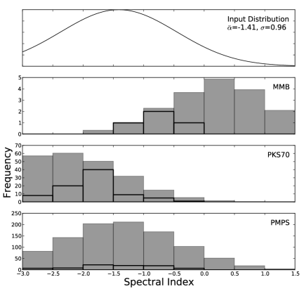
Figure 3: Histograms of the spectral index of detected pulsars in our simulations (grey; averaged over 100 realisations) and from the pulsar catalogue (black outline) for the optimum parameters obtained from Figure 2. The top panel shows the input distribution used to generate a model pulsar population. Note that the spectral index values in the pulsar catalogue are both incomplete, and biased towards those pulsars which have been discovered in early low-frequency surveys.

4.4 Checking for biases in our results

The number of detected pulsars for each survey, as shown in Table 1, was obtained from the most recent version of the ATNF Pulsar Catalogue (Manchester et al., 2005). However, these numbers are by no means absolute — the PMPS survey data have been reprocessed several times (e.g.  Faulkner et al., 2004; Eatough et al., 2010; Mickaliger et al., 2012), each time increasing the recorded number of pulsar detections. Furthermore, the MMB survey yielded its second pulsar discovery only after reprocessing of the data (Bates et al., 2011). Therefore, the numbers shown in Table 2 are lower limits; although the rate of new detections in old data should decrease over time as successively fainter objects are found.

It is important to quantify what impact an increase in the number of detected pulsars in the PMPS, PKS70 and MMB surveys would have on our results. Firstly, to evaluate the impact of further pulsars being discovered in the PKS70 and MMB surveys, the likelihoods ${\cal L}_{\rm MMB}$ and ${\cal L}_{\rm PKS70}$ were recalculated assuming the PKS70 and MMB survey yields increased over the range of 5% to 50%.

In the case where the PMPS survey yield does not change (since such a large number of pulsars have been detected in the survey data, this is not an unreasonable approximation), the calculated values of $\bar{\alpha}$ and $\bar{\sigma}$ do not change significantly as the MMB survey yield increases. As the PKS70 yield is increased, $\bar{\alpha}$ and $\bar{\sigma}$ change by 2 and 3 standard deviations if the yield increases by 15 and 20%, respectively (this corresponds to the discovery of a further 42 and 56 pulsars in the data). Repeating this analysis with the PMPS survey yield increased by 5 and 10% (a large increase on 1038 pulsars) does not change the conclusion — unless the three surveys are all woefully incomplete, $\bar{\alpha}$ and $\bar{\sigma}$ do not deviate significantly from our best-fit values.

5 Alternative Spectral Shapes

5.1 Setting limits on the size of the GPS population

5.1.1 Method & Analysis

The populate code (part of psrpop) was modified to enable the simulation of GPS pulsars. Additional user options were added to specify the fraction, $F$, of pulsars which show GPS behaviour, and to specify the value of the turnover parameter, $a$, in Equation 2.

As the population is generated, $F$ of the pulsars are randomly selected to be GPS sources, but are allocated a flux at 1.4 GHz and a spectral index, $\alpha$, in the usual way. The value of $c$ in Equation 2 may then be calculated (with $x$ defined as in Equation 2) as

$$c=\log_{10}S_{1.4}-ax^{2}-\alpha x$$ (4)

since, as stated earlier, $b$ is considered equivalent to $\alpha$. The flux of the GPS pulsars in the simulation can then be calculated at other frequencies using Equation 2.

Following the procedure used in § 4.1, simulations were performed in order to fill out a grid of $F$ and $a$ values. To reduce the number of variables, the spectral index mean and standard deviation were held fixed at $\alpha=-1.41,\sigma=0.96$, which are the best values from the previous simulations. Again, 500 realisations were performed at each grid point, and a likelihood was calculated in the same way as in § 4.1.

5.1.2 Results

Figure 4 shows the likelihoods calculated from the simulations as a function of $F$ and the turnover parameter, $a$. Significant values for $a$, indicating a severe turnover, are only allowed when $F$ is below $\sim 10\%$. Otherwise, values of $a$ as small as $-0.5$ are allowed in a large fraction, $F\geq 0.40$, of the pulsar population.

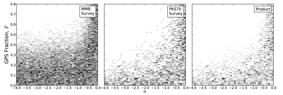
Figure 4: Grey scale plots showing the likelihood (as defined in § 4.2 as a function of the fraction of GPS pulsars in the simulation, $F$, and the turnover parameter used in Equation 2, $a$.

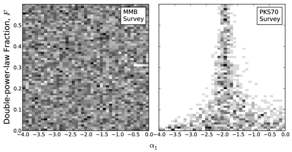
Figure 5: Grey scale plots showing the likelihood (as defined in § 4.2 as a function of the fraction of double-power-law pulsars in the simulation, and the value of $\alpha_{1}$ used. In this case, the product of the likelihoods is unconstrained by the MMB survey, and so resembles the right-hand plot.

5.2 Setting limits of the size of the double-power-law population

5.2.1 Method & Analysis

Further modifications were made to the populate code to allow any given fraction, $F$, of pulsars to have double power-law spectra. As the population is generated, $F$ of the pulsars are randomly selected and given a power-law value, $\alpha_{1}$, to be used at frequencies below 1.4 GHz. The flux density and “high frequency” $\alpha_{2}$ are calculated in the usual way. As in § 5.1.1, simulations were performed, filling out a grid of $F$ and $\alpha_{1}$ values, holding fixed $\alpha_{2}=-1.41,\sigma=0.96$. Again, 500 realisations were performed at each grid point, and a likelihood was calculated in the same way based upon the number of realisations that were able to reproduce the number of detections.

5.2.2 Results

The results from these simulations are shown in Figure 5. The first point of note is that the likelihoods for the MMB survey are not affected by changing values of $\alpha_{1}$, as expected. For the PKS70 survey, though, these two parameters have a substantial impact. We can constrain the population of pulsars with double-power-law spectra to be below $\sim 10\%$ — above this fraction, the value of $\alpha_{1}$ is fixed at $-1.9$, consistent with a single power law (cf. centre panel of Figure 1 for $\sigma=0$). Within this 10% of sources, the value of $\alpha_{1}$ is not well constrained, though shallower spectral indices, $\alpha_{1}>-2$ are favoured.

5.3 Limitations and future work

Having investigated these alternative spectral shapes for pulsars, we are unfortunately not able to place clear constraints upon the size of such populations, or the values of the parameters used to describe their spectral shapes. The only way that such work will be possible is with the results of on-going, and future, surveys at a variety of observing frequencies. Two such on-going pulsar surveys are described below, and in Table 3.

The Green Bank Northern Celestial Cap survey (GBNCC) is an on-going pulsar survey of the Northern sky using the 100-m Green Bank Radio Telescope in West Virginia. Phase 1 of the survey has covered the entire sky with declination $\delta\geq+38\degree$ (Stovall et al. in prep.).

LOFAR is an interferometer based in Europe which is able to observe the sky over two low-frequency bands; one from 30-80 MHz and the other from 110-240 MHz. Simulations for a pulsar survey using LOFAR were first performed by van Leeuwen & Stappers (2010) assuming that the survey would be performed in the higher radio band due to pulse smearing at lower frequencies. These simulations estimated that such a survey with LOFAR would detect $1100\pm 100$ normal pulsars.

With the additional information provided by such large-scale surveys, it may be possible to constrain the size of any population of pulsars with these, or other, alternative spectral shapes.

6 Summary and consequences for pulsar surveys

In § 4 we showed that the relative survey yields of pulsar surveys at three different frequencies can be explained using an underlying spectral-index distribution of pulsars which is Gaussian around a single power law with mean $\bar{\alpha}=-1.41$ and standard deviation $\bar{\sigma}=0.96$. This distribution is both shallower and wider than the values obtained by both Lorimer et al. (1995) and Maron et al. (2000), although in close agreement with measurements made by Malofeev et al. (2000), who calculated values of $\alpha=-1.47,\sigma=0.76$ at observing frequencies of 100-400 MHz. Malofeev et al. (2000) explained the difference between their results and those of Lorimer et al. (1995) and Maron et al. (2000) as a steepening of the spectral index at higher radio frequencies, however, our results suggest this may in fact be due to incompleteness and biases in the samples used.

We showed (see Fig. 3), perhaps not surprisingly, that the detected sample of pulsar spectral index is a strong function of the survey frequency. Surveys carried out at lower frequencies favour the detection of steeper spectrum pulsars compared to experiments carried out at higher frequencies. Thus, although we did not attempt a dynamical study of pulsar evolution, our results imply that any correlations between spectral index and pulsar parameters (such as the observation by Lorimer et al. 1995 that younger pulsars appear to have flatter spectra) needs to be carefully weighed against the survey frequency they have been selected in. Our present results imply that the spectral index–age relationship suggested by Lorimer et al. (1995) is most likely a result of observational selection.

In § 5.1 we investigated the fraction of the pulsar population that could have spectra which peak at a frequency of $\sim 1~{}\mathrm{GHz}$. While the known population of such sources stands at only five (Kijak et al., 2011b), we have shown that a large number of such sources could exist, though only if the turnover parameter is very small, $a=-0.5$. Compared to the smallest measured value, $a=-1.18$ for PSR B1823$-$13, such a small turnover might not be noticed for many pulsars unless they are observed at very low frequencies, for example in the 100 MHz regime.

By allowing the spectral index to take two values, $\alpha_{1}$ below 1.4 GHz and $\alpha_{2}$ above, in § 5.2 we investigated what fraction of pulsars would display a spectral break. We can constrain the population of pulsars for which $\alpha_{1}$ and $\alpha_{2}$ differ significantly to be no more than 10%.

So are we able to place any constraints upon pulsar emission models from our results? Malofeev et al. (1994) and Löhmer et al. (2008) used measured spectral shapes to investigate different models of the pulsar magnetosphere. In so doing, they were required to use spectra with a spectral break. We were unable to place a reasonable constraint upon the values of $\alpha_{1}$ and $\alpha_{2}$ in such a model, and so are unable to rule out such models, or prove them to be valid. However, we have shown that only a small fraction of pulsars should deviate from the model of a spectrum with a constant power-law slope, and therefore future emission models should be able to explain both the size and existence of this sub-population.

Table 3: Observational parameters for the two simulated surveys, the GBNCC survey, and the LOFAR pulsar survey (van Leeuwen & Stappers, 2010).

	GBNCC	LOFAR
Centre frequency (MHz)	350	143
Bandwidth (MHz)	100	47.66
Channel width (MHz)	0.0244	0.012
Gain ($\mathrm{K~{}Jy}^{-1}$)	2.0	5.6
Integration time (s)	120	1020
Sampling interval ($\mu$s)	81.92	1310
Minimum declination (°)	$+38$	$-30$

7 Conclusions

In summary, using simple snapshot models of the pulsar population and a likelihood analysis we have been able to constrain the underlying distribution of spectral indices. We find that the survey yields at three different frequencies can be described by a simple power law spectrum. The distribution of spectral indices is consistent with a normal distribution with a mean of –1.4 and unit standard deviation. Extensions to this simple model were investigated in the form of Gigahertz-peaked spectrum pulsars and we were able to constrain the fraction of such sources in the population as a whole to be at most 10%. A similar fraction of spectra are consistent with being double-power-law. Any models of the pulsar emission mechanism should be able to explain the size and existence of these sub-populations.

Future work to refine this analysis would be to obtain more measurements of existing pulsar spectra. Only a small fraction of the $\sim 2000$ known radio pulsars have had their flux measured at more than one or two observing frequencies. Without more comprehensive flux measurements, it is not possible to constrain the sizes of any populations with non-standard spectral shapes or even to establish the spectral slope. This would allow a more detailed likelihood analysis that accounts for the observed distribution of spectra at each frequency. One aspect that we did not look at in this work, due to the simple snapshot approach taken in our simulations, was the case for any evolution of spectral index with pulsar age. In Lorimer et al. (1995), it was proposed that younger pulsars may have flatter spectra. While our analysis does not directly answer this question, our demonstration that higher frequency surveys tend to select flatter spectrum pulsars suggests that any correlation with age is likely to be weak, since the high-frequency surveys also preferentially select younger pulsars along the Galactic plane. Further observational evidence from large-scale pulsar surveys at several observing frequencies, coupled with observational campaigns to accurately measure pulsar spectral indices, will improve our understanding of the spectral index distribution, and reduce the bias that, from Figure 3, seems to exist in the current catalogues.

References

- Backer & Fisher (1974) Backer D. C., Fisher J. R., 1974, ApJ, 189, 137
- Bates et al. (2011) Bates S. D. et al., 2011, MNRAS, 411, 1575
- Bhat et al. (2004) Bhat N. D. R., Cordes J. M., Camilo F., Nice D. J., Lorimer D. R., 2004, ApJ, 605, 759
- Dembska et al. (2012) Dembska M., Kijak J., Lewandowski W., 2012, ArXiv e-prints (astro-ph/1212.0663)
- Eatough et al. (2010) Eatough R. P., Molkenthin N., Kramer M., Noutsos A., Keith M. J., Stappers B. W., Lyne A. G., 2010, MNRAS, 407, 2443
- Faucher-Giguère & Kaspi (2006) Faucher-Giguère C. A., Kaspi V. M., 2006, ApJ, 643, 332
- Faulkner et al. (2004) Faulkner A. J. et al., 2004, MNRAS, 355, 147
- Izvekova et al. (1981) Izvekova V. A., Kuzmin A. D., Malofeev V. M., Shitov I. P., 1981, Ap&SS, 78, 45
- Kijak et al. (2011a) Kijak J., Dembska M., Lewandowski W., Melikidze G., Sendyk M., 2011a, MNRAS, 418, L114
- Kijak et al. (2011b) Kijak J., Lewandowski W., Maron O., Gupta Y., Jessner A., 2011b, A&A, 531, A16
- Lawson et al. (1987) Lawson K. D., Mayer C. J., Osborne J. L., Parkinson M. L., 1987, MNRAS, 225, 307
- Löhmer et al. (2008) Löhmer O., Jessner A., Kramer M., Wielebinski R., Maron O., 2008, A&A, 480, 623
- Löhmer et al. (2001) Löhmer O., Kramer M., Mitra D., Lorimer D. R., Lyne A. G., 2001, ApJ, 562, L157
- Lorimer (2011) Lorimer D. R., 2011, in Torres D. F., Rea N., ed, High-Energy Emission from Pulsars and their Systems, p. 21
- Lorimer et al. (2006) Lorimer D. R. et al., 2006, MNRAS, 372, 777
- Lorimer et al. (1995) Lorimer D. R., Yates J. A., Lyne A. G., Gould D. M., 1995, MNRAS, 273, 411
- Lyne (2008) Lyne A. G., 2008, in American Institute of Physics Conference Series, Vol. 983, Bassa C., Wang Z., Cumming A., Kaspi V. M., ed, 40 Years of Pulsars: Millisecond Pulsars, Magnetars and More, p. 561
- Malofeev et al. (1994) Malofeev V. M., Gil J. A., Jessner A., Malov I. F., Seiradakis J. H., Sieber W., Wielebinski R., 1994, A&A, 285, 201
- Malofeev & Malov (1980) Malofeev V. M., Malov I. F., 1980, Sov. Astron., 24, 54
- Malofeev et al. (2000) Malofeev V. M., Malov O. I., Shchegoleva N. V., 2000, Astronomy Reports, 44, 436
- Manchester et al. (2005) Manchester R. N., Hobbs G. B., Teoh A., Hobbs M., 2005, AJ, 129, 1993
- Manchester et al. (2001) Manchester R. N. et al., 2001, MNRAS, 328, 17
- Manchester et al. (1996) Manchester R. N. et al., 1996, MNRAS, 279, 1235
- Maron et al. (2000) Maron O., Kijak J., Kramer M., Wielebinski R., 2000, A&A, 147, 195
- Mickaliger et al. (2012) Mickaliger M. B. et al., 2012, ApJ, 759, 127
- Ridley & Lorimer (2010) Ridley J. P., Lorimer D. R., 2010, MNRAS, 404, 1081
- Sieber (1973) Sieber W., 1973, A&A, 28, 237
- Slee et al. (1986) Slee O. B., Alurkar S. K., Bobra A. D., 1986, AuJP, 39, 103
- van Leeuwen & Stappers (2010) van Leeuwen J., Stappers B. W., 2010, A&A, 509, A7