New Concept of Solvability in Quantum Mechanics

Miloslav Znojil

Nuclear Physics Institute ASCR, 250 68 Řež, Czech Republic

Abstract

In a pre-selected Hilbert space ${\cal H}$ of quantum states $|\psi\rangle\in{\cal H}$ the unitarity of the evolution is usually guaranteed via a pre-selection of the generator (i.e., of the Hamiltonian operator $H$) in self-adjoint form, $H=H^{\dagger}$. In fact, the simultaneous use of both of these pre-selections is overrestrictive. One should be allowed to make a given Hamiltonian self-adjoint only after an ad hoc generalization of Hermitian conjugation, $H^{\dagger}\to H^{\ddagger}:=\Theta^{-1}H^{\dagger}\Theta$. We argue that in the generalized, hidden-Hermiticity scenario with nontrivial metric $\Theta\neq I$, the current concept of solvability (meaning, most often, the feasibility of a non-numerical diagonalization of $H$) requires a generalization allowing for a non-numerical form of $\Theta$. A few illustrative solvable quantum models of this type are presented.

PACS 03.65.Db, 03.65.Aa, 05.30.Rt, 02.30.Sa, 03.65.Ca, 11.30.Er, 21.60.Ev, 31.15.xt

1 Introduction

In our recent paper [1] it has been noticed that contrary to the current belief, an active use of an ad hoc variability of the inner products (i.e., in other words, of the freedom of choosing a nontrivial metric $\Theta\neq I$ in the correct physical Hilbert space of quantum states ${\cal H}^{(S)}$ where the superscript ^(S) stands for “standard”) is not restricted to the so called non-Hermitian quantum mechanics and to its characteristic applications in nuclear physics [2] or in molecular physics [3] or in the relativistic quantum kinematical regime [4] or in the ${\cal PT}-$symmetric quantum dynamical regime [5]. In our present paper we intend to develop this idea and to describe some of its consequences in some detail.

From the point of view of the recent history of quantum mechanics it was, certainly, fortunate that in some of the above-mentioned specific hidden-Hermiticity contexts people discovered the advantages of working with such an operator representation $H$ of a given observable quantity (say, of the energy) which only proved Hermitian after a change of the inner product in the initially ill-chosen (i.e., by assumption, unphysical) Hilbert space ${\cal H}^{(F)}$ (the superscript ^(F) might be read here as abbreviating “former”, “first”, “friendly” or, equally well, “false” [6]). Let us emphasize that the shared motivation of many of the above-cited papers speaking about non-Hermitian quantum mechanics resulted just from the observation that several phenomenologically interesting operators (say, Hamiltonians) $H$ appear manifestly non-Hermitian in the “usual” textbook setting and that they only become Hermitian in some much less common representation of the Hilbert space of states.

The amendments of space were, naturally, mediated by the mere introduction of a non-trivial metric $\Theta=\Theta^{(S)}\neq I$ entering the upgraded, $S-$superscripted inner products,

$$\langle\psi_{1}|\psi_{2}\rangle^{(F)}\ \ \to\ \langle\psi_{1}|\psi_{2}\rangle^{(S)}\ :=\langle\psi_{1}|\Theta|\psi_{2}\rangle^{(F)}\,.$$ (1)

Such an inner-product modification changed, strictly speaking, the Hilbert space, ${\cal H}^{(F)}\to{\cal H}^{(S)}$. This had several independent reasons. Besides the formal necessity of re-installing the unitarity of the evolution law, the costs of the transition to the more complicated metric were found more than compensated by the gains due to the persuasive simplicity of Hamiltonian (cf. [2] or [5] in this respect). Moreover, for some quantum systems the transition $F\to S$ may prove motivated by physics itself. The most elementary illustration of such a fundamental reason can be found in our recent study [7] where a consistent simulation of the cosmological phenomenon of quantum Big Bang has been described. In the model the Hamiltonian remained self-adjoint in the false space, $H=H^{\dagger}$. Still, another relevant observable proved non-Hermitian there, $Q\neq Q^{\dagger}$.

Figure 1: Generic domains of parameters for which the metric $\Theta$ exists (upper disc) or for which the spectra of observables $H$ or $Q$ remain potentially observable (the two respective lower discs).

For an entirely general quantum system characterized by two observables $H$ and $Q$, Hermitian or not, a fully universal scenario may be found displayed in Fig. 1. In the picture (where the whole plane symbolizes a multidimensional space of all parameters of the model) we see three circles. Schematically, they represent three boundaries $\partial{\cal D}$ of three domains ${\cal D}$. Thus, the spectrum of $H$ is assumed potentially observable (i.e., real and non-degenerate) in the left lower domain ${\cal D}_{H}$. Similarly, the spectrum of $Q$ is real and non-degenerate inside the right lower domain ${\cal D}_{Q}$. In parallel, the spectrum of the available Hermitizing metrics $\Theta$ must be, by definition, strictly positive (upper circle, domain ${\cal D}_{\Theta}$). In this arrangement, operator $Q$ ceases to represent an observable in domain “I” while operator $H$ ceases to represent an observable in domain “II”. In domain “III”, neither of these two operators can be made Hermitian using the available class of metrics $\Theta$, in spite of the reality of both spectra.

A number of open questions emerges. Some of them will be discussed in our present paper. Via a few illustrative examples we shall show, among other, that and why the variability of the metric $\Theta$ in the physical Hilbert space ${\cal H}^{(S)}$ represents an important merit of quantum theory and that and why the closed-form availability of operator $\Theta$ (i.e., a new form of solvability) is of a truly crucial importance in applications.

2 Methodical guidance: dimension two

2.1 Toy-model Hamiltonian

In the simplest possible two-dimensional and real Hilbert space ${\cal H}^{(F)}\ \equiv\ \mathbb{R}^{2}$ an instructive sample of the time evolution may be chosen as generated by the Hamiltonian (i.e., quantum energy operator or matrix) of Ref. [8],

$$H=H^{(2)}(\lambda)=\left[\begin{array}[]{cc}-1&\lambda\\ -\lambda&1\end{array}\right]\,.$$ (2)

Its eigenvalues $E_{\pm}^{(2)}=\pm\sqrt{1-\lambda^{2}}$ are non-degenerate and real (i.e., in principle, observable) for $\lambda$ inside interval $(-1,1)$. On the two-point domain boundary $\{-1,1\}$, these energies degenerate. Subsequently, they complexify whenever $|\lambda|>1$. In the current literature one calls the boundary points $\lambda=\pm 1$ “exceptional points” (EP, [9]). At these points the eigenvalues degenerate and our toy-model Hamiltonian ceases to be diagonalizable, becoming unitarily equivalent to a triangular Jordan-block matrix,

$$H^{(2)}(1)=\left[H^{(2)}(-1)\right]^{\dagger}=\left[\begin{array}[]{cc}-1&1\\ -1&1\end{array}\right]=$$

$$=\frac{1}{2}\,\left[\begin{array}[]{cr}1&-1\\ 1&1\end{array}\right]\,\left[\begin{array}[]{cc}0&1\\ 0&0\end{array}\right]\,\left[\begin{array}[]{rc}1&1\\ -1&1\end{array}\right]\,.$$

At $|\lambda|>1$, the diagonalizability gets restored but the eigenvalues cease to be real, $E_{\pm}^{(2)}=\pm{\rm i}\,\sqrt{\lambda^{2}-1}$. In the spirit of current textbooks, this leaves these purely imaginary complex conjugate energies unobservable.

2.2 Hidden Hermiticity: The set of all eligible metrics

Our matrix $H^{(2)}(\lambda)$ remains diagonalizable and crypto-Hermitian whenever $-1<\lambda=\sin\alpha<1$, i.e., for the auxiliary Hamiltonian-determining parameter $\alpha$ lying inside a well-defined physical domain ${\cal D}_{H}$ such that $\alpha\in(-\pi/2,\pi/2)$. In such a setting, matrix $H^{(2)}(\lambda)$ becomes tractable as a Hamiltonian of a hypothetical quantum system whenever it satisfies the above-mentioned hidden Hermiticity condition

$$H=H^{\ddagger}:=\Theta^{-1}H^{\dagger}\Theta\,.\$$ (3)

The suitable candidates for the Hilbert-space metric are all easily found from the latter linear equation,

$$\Theta=\Theta^{(2)}_{\lambda}(a,d)=\left[\begin{array}[]{cc}a&b\\ b&d\end{array}\right]\,,\ \ \ \ \ b=-\frac{\lambda}{2}(a+d)\,.$$ (4)

All of their eigenvalues must be real and positive,

$$\theta_{\pm}=\frac{1}{2}\left[a+d\pm\sqrt{(a-d)^{2}+\lambda^{2}(a+d)^{2}}\right]>0\,.$$ (5)

This is satisfied for any positive $\sigma=a+d>0$ and with any real $\delta=a-d$ such that

$$\sqrt{1-\lambda^{2}}=\cos\alpha\ \ >\ \ \frac{\delta}{\sigma}\ \ >\ \,-\sqrt{1-\lambda^{2}}=-\cos\alpha\,.$$ (6)

Without loss of generality we may set $\sigma=2$, put $\delta=\cos\alpha\cos\beta$ and treat the second free parameter $\beta\in(-\pi/2,\pi/2)$ as numbering the admissible metrics

$$\Theta^{(2)}_{(physical)}=\left[\begin{array}[]{cc}1+\cos\alpha\cos\beta&-\sin\alpha\\ -\sin\alpha&1-\cos\alpha\cos\beta\end{array}\right]\,$$ (7)

with eigenvalues

$$\theta_{\pm}=1\pm\sqrt{1-\cos^{2}\alpha\sin^{2}\beta}>0\,.$$ (8)

Thus, all of the eligible physical Hilbert spaces are numbered by two parameters, ${\cal H}^{(S)}={\cal H}^{(S)}(\alpha,\beta)$.

2.3 The second observable $Q=Q^{\ddagger}$

What we now need is the specification of the domain ${\cal D}_{Q}$. For the general four-parametric real-matrix ansatz

$$\tilde{{Q}}=\left[\begin{array}[]{cc}w&x\\ y&z\end{array}\right]\,$$ (9)

the assumption of observability implies that the eigenvalues must be both real and non-degenerate,

$$4xy>-(w-z)^{2}\,.$$ (10)

Once we shift the origin and rescale the units we may set, without loss of generality, $w=-z=-1$. This simplifies the latter condition yielding our final untilded two-parametric ansatz

$${Q}=\left[\begin{array}[]{cc}-1&x\\ y&1\end{array}\right]\,,\ \ \ \ xy>-1\,.$$ (11)

At any fixed metric $\Theta^{(2)}_{(physical)}$ the crypto-Hermiticity constraint (3) imposed upon matrix (11) degenerates to the single relation

$$x-y=2\sin\alpha-(x+y)\cos\alpha\cos\beta\,.$$ (12)

The sum $s=x+y$ may be now treated as the single free real variable which numbers the eligible second observables. The range of this variable should comply with the inequality in Eq. (11). After some straightforward additional calculations one proves that the physical values of our last free parameter remain unrestricted, $s\in\mathbb{R}$, due to the validity of Eq. (12). We may conclude that our example is fully non-numerical. It also offers the simplest nontrivial explicit illustration of the generic pattern as displayed in Fig. 1.

3 Hilbert spaces ${\cal H}^{(F)}$ of dimension $N$

3.1 Anharmonic Hamiltonians

During the developments of mathematics for quantum theory, one of the most natural paths of research started from the exactly solvable harmonic-oscillator potential $V^{(HO)}(x)=\omega^{2}x^{2}$ and from its power-law perturbations $V^{(AHO)}(x)=\omega^{2}x^{2}+g\,x^{m}$. Perturbation expansions of energies proved available even at the “unusual”, complex values of the coupling constants $g\notin\mathbb{R}^{+}$. The particularly interesting mathematical results have been obtained at $m=3$ and at $m=4$. In physics and, in particular, in quantum field theory the climax of the story came with the letter [10] where, under suitable ad hoc boundary conditions and constraints upon $g=g(m)$ (called, conveniently, ${\cal PT}-$symmetry), the robust reality (i.e., in principle, observability) of the spectrum has been achieved at any real exponent $m>2$ even for certain unusual, complex values of the coupling.

It has been long believed that the ${\cal PT}-$symmetric Hamiltonians $H=H(m)$ with real spectra are all consistent with the postulates of quantum theory, i.e., that these operators are crypto-Hermitian, i.e., Hermitian in the respective Hamiltonian-adapted Hilbert spaces ${\cal H}^{(S)}(m)$ [5]. Due to the ill-behaved nature of the wave functions at high excitations, unfortunately, such a simple-minded physical interpretation of these models has been shown contradictory [11]. On these grounds one has to develop some more robust approaches to the theory for similar models in the nearest future.

In our present paper we shall avoid such a danger by recalling the original philosophy of Scholtz et al [2]. They simplified the mathematics by admitting, from the very beginning, that just the bounded-operator and/or discrete forms of the eligible anharmonic-type toy-model Hamiltonians $H\neq H^{\dagger}$ should be considered.

3.2 Discrete Hamiltonians

For our present illustrative purposes we intend to recall, first of all, one of the most elementary versions of certain general, $N-$dimensional matrix analogues of the differential toy-model Hamiltonians, which were proposed in Refs. [8]. Referring to the details as described in that paper, let us merely recollect that these Hamiltonians are defined as certain tridiagonal and real matrices $H^{(N)}=H_{0}^{(N)}+V^{(N)}$ where the “unperturbed”, harmonic-oscillator-simulating main diagonal remains equidistant, $H^{(N)}_{11}=(H_{0}^{(N)})_{11}=-N+1$, $H^{(N)}_{22}=(H_{0}^{(N)})_{22}=-N+3$, …, $H^{(N)}_{NN}=(H_{0}^{(N)})_{NN}=N-1$ while the off-diagonal “perturbation” becomes variable and, say, antisymmetric, $V^{(N)}_{12}=-V^{(N)}_{21}$, $V^{(N)}_{23}=-V^{(N)}_{32}$, …$V^{(N)}_{N-1N}=-V^{(N)}_{NN-1}$. The word “perturbation” is written here in quotation marks because, in the light of results of Ref. [12], the spectral properties of the model become most interesting in the strongly non-perturbative regime where one up-down symmetrizes and re-parametrizes the perturbation $V^{(N)}_{k,k+1}=-V^{(N)}_{k+1,k}=$

$$=\sqrt{k(N-k)(1-t-t^{2}-\ldots-t^{J-1}-G_{k}t^{J})}\,,$$

$$\ \ \ \ \ \ \ \ \ \ \ \ \ \ N=2J\ {\rm or}\ N=2J+1\,.$$

This parametrization proved fortunate in the sense that it enabled us to replace the usual numerical analysis by a rigorous computer-assisted algebra. In this sense, the model in question appeared to represent a sort of an exactly solvable model, precisely in the spirit of our present message.

The new parameter $t\geq 0$ is auxiliary and redundant. It may be interpreted, say, as a measure of distance of the system from the boundary $\partial{\cal D}_{H}$ of the domain of spectral reality. At very small $t$ the local part of boundary $\partial{\cal D}_{H}$ has been shown to have the most elementary form of two parallel hyperplanes in the $J-$dimensional space of parameters $G_{n}$ [12].

In the simplest nontrivial special case of $N=2$ the present Hamiltonian $H^{(N)}$ degenerates precisely to the above-selected toy-model of section 2. Vice versa, the basic components of the $N=2$ discussion (i.e., first of all, the feasibility of the construction of the metric and of the second observable) might be immediately transferred to all $N>2$. Several steps in this direction may be found performed in our recent paper on the solvable benchmark simulations of the phase transitions interpreted as a spontaneous ${\cal PT}-$symmetry breakdown [13].

4 The problem of non-uniqueness of the ad hoc metric $\Theta=\Theta({H})$

The roots of the growth of popularity of the description of stable quantum systems using representations of observables which are non-Hermitian in an auxiliary Hilbert space ${\cal H}^{(F)}$ may be traced back not only to the entirely abstract mathematical analyses of spectra of quasi-Hermitian operators [14] and of the operators which are self-adjoint in the so called Krein spaces with indefinite metric [15] but also to the emergence of manageable non-Hermitian models in quantum field theory [16] or even in classical optics [17], etc.

After a restriction of attention to quantum theory, the key problem emerges in connection with the ambiguity of the assignment $H\to\Theta(H)$ of the physical Hilbert space ${\cal H}^{(S)}$ to a given generator $H$ of time evolution. For many phenomenologically relevant Hamiltonians $H$ it appeared almost prohibitively difficult to define and construct at least some of the eligible metrics $\Theta=\Theta(H)$ in an at least approximate form (cf., e.g., Ref. [18] in this respect). Clearly, in methodical analyses the opportunity becomes wide open to finite-dimensional and solvable toy models.

4.1 Solvable quantum models with more than one observable

Let us restrict the scope of this paper to the quantum systems which are described by a Hamiltonian $H=H(\lambda)$ accompanied by a single other operator $Q=Q(\varrho)$ representing a complementary measurable quantity like, e.g., angular momentum or coordinate. In general we shall assume that symbols $\lambda$ and $\varrho$ represent multiplets of coupling strengths or of any other parameters with an immediate phenomenological or purely mathematical significance. We shall also solely work here with the finite-dimensional matrix versions of our operators of observables.

In such a framework it becomes much less difficult to analyze one of the most characteristic generic features of crypto-Hermitian models which lies in their “fragility”, i.e., in their stability up to the point of a sudden collapse. Mathematically, we saw that the change of the stability/instability status of the model is attributed to the presence of the exceptional-point horizons in the parametric space. In the context of phenomenology, people often speak about the phenomenon of quantum phase transition [17].

Let us now return to Fig. 1 where the set of the phase-transition points pertaining to the Hamiltonian $H$ is depicted as a schematic circular boundary $\partial{\cal D}_{H}$ of the left lower domain inside which the spectrum of $H$ is assumed, for the sake of simplicity, non-degenerate and completely real. Similarly, the right lower disc or domain ${\cal D}_{Q}$ is assigned to the second observable $Q$. Finally, the upper, third circular domain ${\cal D}_{\Theta}$ characterizes the parametric subdomain of the existence of a suitable general or, if asked for, special class of the eligible candidates $\Theta$ for a physical metric operator. The key message delivered by Fig. 1 is that at any $N$, the correct physics may still only be formulated inside the subdomain ${\cal D}={\cal D}_{H}\bigcap{\cal D}_{H}\bigcap{\cal D}_{H}$. A generalization of this scheme to systems with more observables, $Q\to Q_{1}$, $Q_{2}$, …  would be straightforward.

4.2 Quantum observability paradoxes

One of the most exciting features of all of the above-mentioned models may be seen in their ability of connecting the stable and unstable dynamical regimes, within the same formal framework, as a move out of the domain ${\cal D}$ though one of its boundaries. In this sense, the exact solvability of the $N<\infty$ toy models proves crucial since the knowledge of the boundary $\partial{\cal D}_{\Theta}$ remains practically inaccessible in the majority of their $N=\infty$ differential-operator alternatives [18].

In the current literature on the non-Hermitian representations of observables, people most often discuss just the systems with a single relevant observable $H(\lambda)$ treated, most often, as the Hamiltonian. In such a next-to-trivial scenario it is sufficient to require that operator $H$ remains diagonalizable and that it possesses a non-degenerate real spectrum. Once we add another observable $Q$ into considerations, the latter conditions merely specify the interior of the leftmost domain ${\cal D}_{H}$ of our diagram Fig. 1.

One may immediately conclude that the physical predictions provided by the Hamiltonian alone (and specifying the physical domain of stability as an overlap between ${\cal D}_{H}$ and the remaining upper disc or domain ${\cal D}_{\Theta}$) remain heavily non-unique in general. According to Scholtz et al [2] it is virtually obligatory to take into account at least one other physical observable $Q=Q(\varrho)$, therefore.

In opposite direction, even the use of a single additional observable $Q$ without any free parameters may prove sufficient for an exhaustive elimination of all of the ambiguities in certain models [5]. One can conclude that the analysis of the consequences of the presence of the single additional operator $Q=Q(\varrho)$ deserves a careful attention. At the same time, without the exact solvability of the models, some of their most important merits (like, e.g., the reliable control and insight in the processes of the phase transitions) might happen to be inadvertently lost.

5 Adding the degrees of freedom

5.1 Embedding: $N=2$ space inside $N=3$ space

In the spirit of Ref. [19] a return to observability may be mediated by an enlargement of the Hilbert space. For example, a weak-coupling immersion of our matrices $H^{(2)}(\lambda)$ in their three by three extension

$$H^{(3)}=\left[\begin{array}[]{ccc}-1&1+z&0\\ \vskip 6.0pt plus 2.0pt minus 2.0pt\cr-1-z&1&g\\ \vskip 6.0pt plus 2.0pt minus 2.0pt\cr 0&-g&3\end{array}\right]$$ (13)

may be interpreted as a consequence of the immersion of the smaller Hilbert space (where one defined Hamiltonian (2)) into a bigger Hilbert space. Via the new Hamiltonian (13), the old Hamiltonian becomes weakly coupled to a new physical degree of freedom by the interaction proportional to a small constant $g$.

In a way discussed in more detail in our older paper [20], the boundary of the new physical domain ${\cal D}_{H^{(3)}}$ coincides with the zero line of the following polynomial $G(z,g)$ in two variables,

$$60\,{g}^{2}{z}^{2}-6\,z{g}^{4}-12\,{g}^{2}{z}^{3}-{z}^{6}-162\,z+27\,{g}^{2}-18\,{g}^{4}-{g}^{6}-$$

$$-153\,{z}^{2}-3\,{g}^{4}{z}^{2}-3\,{g}^{2}{z}^{4}-6\,{z}^{5}-30\,{z}^{4}-80\,{z}^{3}+144\,z{g}^{2}.$$

The shape of this line is shown in Fig. 2.

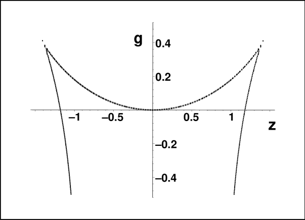
Figure 2: The boundary of the domain of reality of the spectrum of Hamiltonian (13) in $z-g$ plane (i. e., the zero line of polynomial $G(z,g)$).

In the vicinity of $z=0$ and $g=0$, the truncated polynomial $G_{0}(z,g)=27\,{g}^{2}-162\,z-18\,{g}^{4}+144\,z{g}^{2}-{g}^{6}-153\,{z}^{2}-6\,z{g}^{4}$ appears useful as a source of the auxiliary boundary of a fairly large subdomain ${\cal D}_{0}$ of the physical domain ${\cal D}_{H^{(3)}}$ (cf. Fig. (3)).

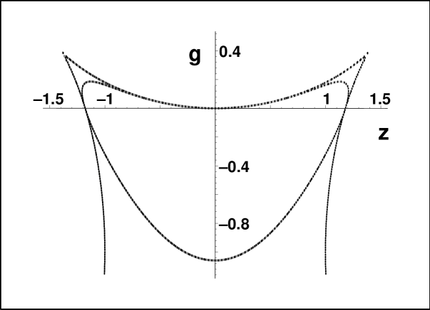
Figure 3: The comparison of zero lines of functions $G_{0}(z,g)$ and $G(z,g)$.

All of these observations imply that the original $z=0$ boundary bends up, i.e., the net effect of the introduction of the new, not too large coupling $g\neq 0$ lies in the enlargement of the domain of the reality of the energy spectrum beyond $\lambda=1$ (and, symmetrically, below $\lambda=-1$). In other words, an enhancement of the stability of the system with respect to some random perturbations is achieved simply by its coupling to an environment.

5.2 Global metrics at $N=3$

Figure 4: The subdominant eigenvalue of metric $\Theta^{(3)}(1,1,1)$. It stays safely positive in the whole preselected rectangle of parameters $z$ and $s$.

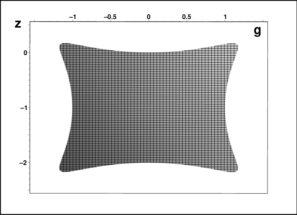
Figure 5: The complete domain of positivity of the smallest eigenvalue of metric $\Theta^{(3)}(1,1,1)$.

The enlarged system controlled by Hamiltonian $H^{(3)}$ of Eq. (13) has been chosen as crypto-Hermitian. The construction of the eligible metrics

$$\Theta^{(3)}=\left[\begin{array}[]{ccc}a&b&c\\ \vskip 6.0pt plus 2.0pt minus 2.0pt\cr b&f&h\\ \vskip 6.0pt plus 2.0pt minus 2.0pt\cr c&h&m\end{array}\right]$$ (14)

of the enlarged and re-coupled system may be perceived as another exercise in the construction of the metrics exactly, by non-numerical means. Using the similar techniques we obtain, step-by-step,

$$c=(-h-h\,z-b\,g)/4,$$

$$b=-(4\,a\,z+4\,f+4\,f\,z+4\,a+h\,g+g\,h\,z)/(8+g^{2})$$

and eliminate, finally, $-2h\,(9+2\,z+z^{2}+g^{2})/g=$

$$=-2\,a\,z-a\,z^{2}+7\,f-2\,f\,z-f\,z^{2}-a+8\,m+m\,g^{2}+f\,g^{2}.$$

Thus, starting from the three arbitrary real parameters $\Theta_{11}=a$, $\Theta_{22}=f$ and $\Theta_{33}=m$ we recursively eliminate $\Theta_{1,3}=c=(-h-h\,z-b\,g)/4$, $\Theta_{1,2}=b=-(4\,a\,z+4\,f+4\,f\,z+4\,a+h\,g+g\,h\,z)/(8+g^{2})$ and $\Theta_{2,1}=h=-1/2\,g\,(-2\,a\,z-a\,z^{2}+7\,f-2\,f\,z-f\,z^{2}-a+8\,m+m\,g^{2}+f\,g^{2})/(9+2\,z+z^{2}+g^{2})$. As a final result we obtain the formula for

$$2\,(9+2\,z+{z}^{2}+{g}^{2})\,\Theta_{1,2}=$$

$$=z{g}^{2}m+fz{g}^{2}+m{g}^{2}+f{g}^{2}-3\,f{z}^{2}-3\,a{z}^{2}-$$

$$-f{z}^{3}-a{z}^{3}-9\,a-11\,fz-11\,az-9\,f\,.$$

Thus, we may denote $\Theta=\Theta^{(3)}(a,f,m)$ and conclude that the metric is obtainable in closed form so that our extended, $N=3$ quantum system remains also solvable.

If we also wish to determine the critical boundaries $\partial{\cal D}_{\Theta}$ of the related metric-positivity domain ${\cal D}_{\Theta}$, the available Cardano’s closed formulae for the corresponding three eigenvalues $\theta_{j}$ yield just the correct answer in a practically useless form. Thus, we either have to recall the available though still rather complicated algebraic boundary-localization formulae of Ref. [20] or, alternatively, we may simplify the discussion by the brute-force numerical localization of a sufficiently large metric-supporting subdomain in the parametric space. For the special choice of $a=f=m=1$ we found, for example, that for the sufficiently large range of parameters $z$ and $g$ as chosen in Figs. 4 and  5 we reveal that while the two upper eigenvalues $\theta_{2}$ and $\theta_{1}$ remain safely positive, the minimal eigenvalue $\theta_{0}$ only remains positive inside the minimal domain of positivity as displayed in Fig. 5. Thus, the boundary of the latter domain represents an explicit concrete realization of its abstract upper-circle representative in Fig. 1.

6 Up-down symmetrized couplings to the environment

6.1 Toy model with $N=9$

The $\cal PT-$symmetric and tridiagonal nine-by-nine-matrix Hamiltonian $H^{(9)}$ of Ref. [8] reads

$$\left[\begin{array}[]{ccccccccc}-8&b&0&0&0&0&0&0&0\\ -b&-6&c&0&0&0&0&0&0\\ 0&-c&-4&d&0&0&0&0&0\\ 0&0&-d&-2&{\alpha}&0&0&0&0\\ 0&0&0&-{\alpha}&0&{\alpha}&0&0&0\\ 0&0&0&0&-{\alpha}&2&d&0&0\\ 0&0&0&0&0&-d&4&c&0\\ 0&0&0&0&0&0&-c&6&b\\ 0&0&0&0&0&0&0&-b&8\end{array}\right]\,.$$

In the limit $\alpha\to 0$ it splits into a central one-dimensional submatrix with eigenvalue $0$ and a pair of non-trivial four-by-four sub-Hamiltonians $H^{(4)}$. The spectrum remains real, say, for the family of parameters $b=\sqrt{3+3t}$, $c=2\sqrt{1+t}$ and $d=\sqrt{3+3t}$. They span an interval in the physical domain ${\cal D}_{H}$ whenever $t$ stays negative, $t\in(-\infty,0)$ [12].

At $\alpha=0$ the special and easily seen feature of the latter operator (i.e., matrix) is that at $t=0$ (i.e., at the boundary of its physical domain ${\cal D}_{H}$) it ceases to represent an observable because its eigenvalues degenerate. Indeed, the vanishing level $E_{4}=0$ separates from the two degenerate quadruplets of $E_{4+j}=-E_{4-j}=5$ with $j=1,2,3,4$. Subsequently, at $t>0$, these eigenvalues get, up to the constantly real level $E_{4}=0$, complex. This makes the model suitable for quantitative studies of the properties of the boundary $\partial{\cal D}_{H}$ [13].

6.2 Boundary $\partial{\cal D}_{H}$

The $t-$independent level $E_{4}=0$ is a schematic substitute for a generic environment. Each of the two remaining subsystems remains coupled to this environment by the coupling or matrix element ${\alpha}$. We shall choose its value as proportional to $t$ via a not too large real coupling constant $\beta$, ${\alpha}=\beta\,t$.

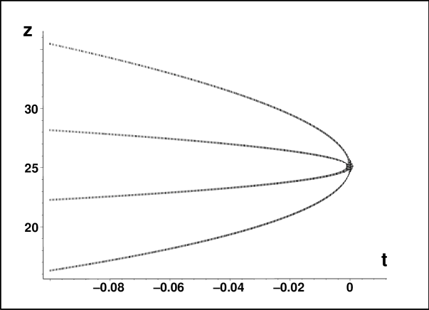
Figure 6: The $t-$dependence of the real roots $z_{j}$ of secular equation (15). The collapse at $t=0$ is not destroyed due to the weakness of the coupling to the environment ($\beta=1$).

At the particular choice of $\beta=1$ the description of the boundary $\partial{\cal D}_{H}$ remains feasible by non-numerical means yielding the transparent and algebraically tractable secular equation

$$0=z^{4}+\left(-100-20\,t+2\,{t}^{2}\right)z^{3}+$$

$$+\left(3750+500\,t-80\,{t}^{2}-34\,{t}^{3}\right)z^{2}+$$ (15)

$$+\left(-62500+12500\,t+4810\,{t}^{2}+360\,{t}^{3}+158\,{t}^{4}\right)z+$$

$$+390625-312500\,t-23500\,{t}^{2}+22450\,{t}^{3}-3221\,{t}^{4}-126\,{t}^{5}$$

which may very easily be treated numerically. Obviously, the level $E_{4}=0$ separates while the other two quadruplets acquire the square-root form $E_{4+j}=-E_{4-j}=\sqrt{z_{j}}$ for $j=1,2,3,4$. Hence, one may proceed and study the spectrum of $z=E^{2}$ in full parallel with our above $N=3$ model.

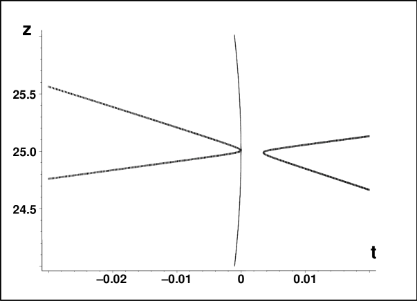
Figure 7: The $t-$dependence of the real roots $z_{j}$ of secular equation (15) near $t=0$ at $\beta=2.73$. The collapse survives, a partial recovery emerges at negative $t$.

The $\beta=1$ results are sampled in Fig. 6. Inside the physical domain of $t<0$, qualitatively the same pattern is still obtained even at the perceivably larger $\beta=2.73$ (cf. Fig. 7). Once we are now getting very close to the critical value of $\beta\approx 2.738$, the situation becomes unstable. In the unphysical domain of $t>0$, for example, we can spot an anomalous partial de-complexification of the energies at certain positive values of parameter $t$.

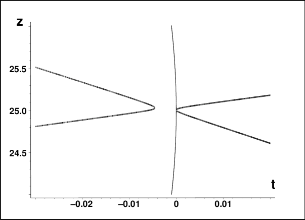
Figure 8: The change of the $t-$dependence of the real roots $z_{j}$ of secular equation (15) near $t=0$ at $\beta=2.75$.

At cca $\beta\approx 2.738$ the two separate EP instants of the degeneracy and complexification/decomplexification of the energies fuse themselves. Subsequently, a qualitatively new pattern emerges. Its graphical sample is given in Fig. 8. First of all, the original multiple EP collapse gets decoupled. This implies that at $\beta=2.75$ as used in the latter picture, the inner two levels degenerate and complexify at a certain small but safely negative $t=t_{crit}\approx-0.004$. Due to the solvability of the model we may conclude that the boundary-curve $\partial{\cal D}_{H}$ starts moving with parameter $\beta$.

7 Non-Hermitian quantum graphs

7.1 Models with point interactions

Another interesting ${\cal PT}-$symmetric single-particle differential-operator Hamiltonian $H$ with the property $H\neq H^{\dagger}$ in ${\cal H}^{(F)}$ has been proposed in Ref. [21]. The particle of mass $\mu=1/2$ has been assumed there living on a finite interval of $x\in(-L,L)$. The only nontrivial interaction was chosen as localized at the endpoints and characterized by the Robin-type boundary conditions

$$\Psi^{\prime}(\pm L)+i\alpha\;\!\Psi(\pm L)=0\,,\ \ \ \ \alpha>0\,\ \ \ \ 2L\alpha/\pi\neq 1,2,\ldots\,.$$ (16)

The extreme simplicity of this model opened the way not only towards the elementary formula for the energy spectrum,

$$E_{0}=\alpha^{2}\,,\ \ \ E_{n}=\left(\frac{n\pi}{2L}\right)^{2}\,,\ \ \ n=1,2,\ldots\,$$ (17)

but also towards the equally elementary construction of the complete family of the eligible metrics $\Theta$ (cf., e.g., Refs. [22] for the details).

The solvability as well as extreme simplicity of this model proved encouraging in several directions. In the present context, the mainstream developments may be seen in the study of its discrete descendants (cf. the next subsection). Nevertheless, before turning our attention to the resulting family of the finite-dimensional crypto-Hermitian problems, let us add a brief remark on the alternative possibility of a transfer of the present analysis of the idea of generalized solvability to the quickly developing field of so called quantum graphs, i.e., of systems where the usual underlying concept of a point particle moving along a real line or interval is generalized in the sense that the single interval (say, $e_{+}:=(0,L)$) is replaced by a suitable graph $\mathbb{G}^{(q)}$ composed of $q$ edges $e_{j}$, $j=0,1,\ldots,q-1$.

The idea still waits for its full understanding and consistent implementation. In particular, in Ref. [23] we showed that even for the least complicated equilateral $q-$pointed star graphs with $q>2$ the spectrum of energies need not remain real anymore, even if one parallels, most closely, the $q=2$ boundary conditions (16) and even if one does not attach any interaction to the central vertex. In our present notation this means that the domain ${\cal D}_{H}$ of Fig. 1 becomes empty. In other words, the applicability of this and similar models remains restricted to classical physics and optics while a correct, widely acceptable quantum-system interpretation of the manifestly non-Hermitian $q>2$ quantum graphs must still be found in the future.

7.2 Discrete lattices

As we already indicated above, one of the most promising methods of an efficient suppression of some of the above-mentioned shortcomings of the ${\cal PT}-$symmetric models which are built in an infinite-dimensional Hilbert space ${\cal H}^{(F)}$ may be seen in the transition, say, to the discrete analogues and descendants of various confining ${\cal PT}-$symmetric as well as non$-{\cal PT}-$symmetric potentials [24]. In particular, the most elementary discrete analogues of the most elementary end-point-interaction-simulating boundary conditions (16) may be seen in the suitable end-point non-Hermitian perturbations $W^{(N)}$ of the standard Hermitian kinetic-energy matrices $-\triangle^{(N)}$, i.e., of the $N$ by $N$ negative discrete Laplacean Hamiltonians where mere two diagonals of matrix elements are non-vanishing, $\triangle^{(N)}_{k,k+1}=\triangle^{(N)}_{k+1,k}=1$, $k=1,2,\ldots,N-1$.

With this idea in mind we already studied, in Ref. [25], the most elementary model with

$${W}^{(N)}({\lambda})=\left[\begin{array}[]{cccccc}0&-{\it{\lambda}}&0&0&\ldots&0\\ {}{\it{\lambda}}&0&0&0&\ddots&\vdots\\ {}0&0&0&\ddots&\ddots&0\\ {}0&0&\ddots&\ddots&0&0\\ {}\vdots&\ddots&\ddots&0&0&{\it{\lambda}}\\ {}0&\ldots&0&0&-{\it{\lambda}}&0\end{array}\right]\,.$$ (18)

We succeeded in constructing the complete $N-$parametric family of the physics-determining solutions $\Theta$ of the compatibility constraint (3). In Ref. [26] we then extended these results to the more general, multiparametric boundary-condition-simulated perturbations

$${W}^{(N)}({\lambda,\mu})=\left[\begin{array}[]{cccccccc}0&-{\it{\lambda}}&0&0&\ldots&&\ldots&0\\ {}{\it{\lambda}}&0&{\it{\mu}}&0&\ldots&&\ldots&0\\ {}0&-{\it{\mu}}&0&0&\ddots&&&\vdots\\ {}0&0&0&0&\ddots&\ddots&&\vdots\\ {}\vdots&&\ddots&\ddots&\ddots&0&0&0\\ {}\vdots&&&\ddots&0&0&-{\it{\mu}}&0\\ {}0&\ldots&&\ldots&0&{\it{\mu}}&0&{\it{\lambda}}\\ {}0&\ldots&&\ldots&0&0&-{\it{\lambda}}&0\end{array}\right]\,$$ (19)

etc. Thus, all of these models may be declared solvable in the presently proposed sense. At the same time, the question of the survival of feasibility of these exhaustive constructions of metrics $\Theta$ after transition to nontrivial discrete quantum graphs remains open [27].

8 Discussion

During transitions from classical to quantum theory one must often suppress various ambiguities – cf., e.g., the well known operator-ordering ambiguity of Hamiltonians which are, classically, defined as functions of momentum and position. Moreover, even after we specify a unique quantum Hamiltonian operator $H$, we may still encounter another, less known ambiguity which is well know, e.g., in nuclear physics [2]. The mathematical essence of this ambiguity lies in the freedom of our choice of a sophisticated conjugation ${\cal T}^{(S)}$ which maps the standard physical vector space ${\cal V}$ (i.e., the space of ket vectors $|\psi\rangle$ representing the admissible quantum states) onto the dual vector space ${\cal V}^{\prime}$ of the linear functionals over ${\cal V}$. In our present paper we discussed some of the less well known aspects of this ambiguity in more detail. Let us now add a few further comments on the current quantum-model building practice.

First of all, let us recollect that one often postulates a point-particle (or point-quasi-particle) nature and background of the generic quantum models. Thus, in spite of the existence of at least nine alternative formulations of the abstract quantum mechanics as listed, by Styer et al, in their 2002 concise review paper [28], a hidden reference to the wave function $\psi(x)$ which defines the probability density and which lives in some “friendly” Hilbert space (say, in ${\cal H}^{(F)}=L^{2}(\mathbb{R}^{d})$) survives, more or less explicitly, in the large majority of our conceptual as well as methodical considerations.

A true paradox is that the simultaneous choice of the friendly Hilbert space ${\cal H}^{(F)}$ and of some equally friendly differential-operator generator $H=\triangle+V(x)$ of the time evolution encountered just a very rare critical opposition in the literature [29]. The overall paradigm only started changing when the nuclear physicists imagined that the costs of keeping the Hilbert space ${\cal H}^{(F)}$ (or, more explicitly, its inner product) unchanged may prove too high, say, during variational calculations [2]. Anyhow, the ultimate collapse of the old paradigm came shortly after the publication of the Bender’s and Boettcher’s letter [10] in which, for certain friendly ODE Hamiltonians $H=\triangle+V(x)$ the traditional choice of space ${\cal H}^{(F)}=L^{2}(\mathbb{R})$ has been found unnecessarily over-restrictive (the whole story may be found described in [5]).

The net result of the new developments may be summarized as an acceptability of a less restricted input dynamical information about the system. In other words, the use of the friendly space ${\cal H}^{(F)}$ in combination with a friendly Hamiltonian $H=H^{\dagger}$ has been found a theoretician’s luxury. The need of a less restrictive class of standard Hilbert spaces ${\cal H}^{(S)}$ which would differ from their “false” predecessor ${\cal H}^{(F)}$ by a nontrivial inner-product metric $\Theta\neq I$ appeared necessary.

One need not even abandon the most common a priori selection of the friendly Hilbert space ${\cal H}^{(F)}$ of the ket vectors $|\psi\rangle$ with their special Dirac’s duals (i.e., roughly speaking, with the transposed and complex conjugate bra vectors $\langle\psi|$) yielding the Dirac’s inner product $\langle\psi_{1}|\psi_{2}\rangle=\langle\psi_{1}|\psi_{2}\rangle^{(F)}$. What is only new is that such a pre-selected, $F-$superscripted Hilbert space need not necessarily retain the usual probabilistic interpretation.

One acquires an enhanced freedom of working with a sufficiently friendly form of the input Hamiltonian $H$, checking solely the reality of its spectrum. Thus, one is allowed to admit that $H\neq H^{\dagger}$ in ${\cal H}^{(F)}$. One must only introduce, on some independent initial heuristic grounds, the amended Hilbert space ${\cal H}^{(S)}$. For such a purpose it is sufficient to keep the same ket-vector space and just to endow it with some sufficiently general and Hamiltonian-adapted (i.e., Hamiltonian-Hermitizing) inner product (1) [2]. This is the very core of innovation. In the physical Hilbert space ${\cal H}^{(S)}$ the unitarity of the evolution of the system must remain guaranteed, as usual, by the Hermiticity of our Hamiltonian in this space, i.e., by a hidden Hermiticity condition

$$H=\Theta^{-1}H^{\dagger}\Theta:=H^{\ddagger}\,$$ (20)

alias crypto-Hermititicity condition [6]. In the special case of finite matrices one speaks about the quasi-Hermiticity condition. Unfortunately, the latter name becomes ambiguous and potentially misleading whenever one starts contemplating certain sufficiently wild operators in general Hilbert spaces [14].

It is rarely emphasized (as we did in [1]) that the choice of the metric remains an inseparable part of our model-building duty even if our Hamiltonian happens to be Hermitian, incidentally, also in the unphysical initial Hilbert space ${\cal H}^{(F)}$. Irrespectively of the Hermiticity or non-Hermiticity of $H$ in auxiliary ${\cal H}^{(F)}$, one must address the problem of the independence of the dynamical input information carried by the metric $\Theta$. Only the simultaneous specification of the operator pair of $H$ and $\Theta$ connected by constraint (20) defines physical predictions in consistent manner. In this sense, the concept of solvability must necessarily involve also the simplicity of $\Theta$.

Acknowledgements

Work supported by GAČR, grant Nr. P203/11/1433.

References

- [1] M. Znojil and H. B. Geyer. Smeared quantum lattices exhibiting PT-symmetry with positive P. Fortschr Physik 61(2-3): 111–123, 2013.
- [2] F. G. Scholtz, H. B. Geyer and F. J. W. Hahne. Quasi-Hermitian Operators in Quantum Mechanics and the Variational Principle. Ann Phys (NY) 213: 74–101, 1992.
- [3] N. Moiseyev. Non-Hermitian Quantum Mechanics. CUP, Cambridge, 2011.
- [4] M. Znojil. Relativistic supersymmetric quantum mechanics based on Klein-Gordon equation. J Phys A: Math Gen 37: 9557–9571, 2004; V. Jakubsky and J. Smejkal. A positive-definite scalar product for free Proca particle. Czech J Phys 56: 985, 2006; F. Zamani and A. Mostafazadeh. Quantum Mechanics of Proca Fields. J Math Phys 50: 052302, 2009.
- [5] C. M. Bender. Making sense of non-Hermitian Hamiltonians. Rep Prog Phys 70: 947–1018, 2007.
- [6] M. Znojil. Three-Hilbert-space formulation of Quantum Mechanics. SIGMA 5: 001, 2009 (arXiv overlay: 0901.0700).
- [7] M. Znojil. Quantum Big Bang without fine-tuning in a toy-model. J Phys: Conf Ser 343: 012136, 2012.
- [8] M. Znojil. Maximal couplings in PT-symmetric chain-models with the real spectrum of energies. J Phys A: Math Theor 40: 4863–4875, 2007.
- [9] T. Kato. Perturbation theory for linear operators. Springer, Berlin, 1966.
- [10] C. M. Bender and S. Boettcher. Real spectra in non-Hermitian Hamiltonians having PT symmetry. Phys Rev Lett 80: 5243–5246, 1998.
- [11] P. Siegl and D. Krejcirik, On the metric operator for the imaginary cubic oscillator. Phys. Rev. D 86: 121702(R), 2012.
- [12] M. Znojil. Tridiagonal PT-symmetric N by N Hamiltonians and a fine-tuning of their observability domains in the strongly non-Hermitian regime. J Phys A: Math Theor 40: 13131–13148, 2007.
- [13] M. Znojil. Quantum catastrophes: a case study. J Phys A: Math Theor 45: 444036, 2012.
- [14] J. Dieudonne. Quasi-Hermitian operators. Proc Int Symp Lin Spaces, Pergamon, Oxford, 1961, pp. 115–122.
- [15] H. Langer and Ch. Tretter. A Krein space approach to PT symmetry. Czechosl J Phys 54: 1113–1120, 2004; P. Siegl. Non-Hermitian quantum models, indecomposable representations and coherent states quantization. Univ. Paris Diderot & FNSPE CTU, Prague, 2011 (PhD thesis).
- [16] C. M. Bender and K. A. Milton. Nonperturbative calculation of symmetry breaking in quantum field theory. Phys Rev D 55: 3255–3259, 1997.
- [17] C. E. Rüter, R. Makris, K. G. El-Ganainy, D. N. Christodoulides, M. Segev and D. Kip, Observation of parity-time symmetry in optics. Nature Phys 6: 192, 2010.
- [18] A. Mostafazadeh. Metric Operator in Pseudo-Hermitian Quantum Mechanics and the Imaginary Cubic Potential. J Phys A: Math Gen 39: 10171–10188, 2006.
- [19] M. Znojil. A return to observability near exceptional points in a schematic PT-symmetric model. Phys Lett B 647: 225–230, 2007.
- [20] M. Znojil. Horizons of stability. J Phys A: Math Theor 41: 244027, 2008.
- [21] D. Krejcirik, Hynek Bila and M. Znojil. Closed formula for the metric in the Hilbert space of a PT-symmetric model. J Phys A: Math Gen 39: 10143–10153, 2006.
- [22] J. Železný. The Krein-space theory for non-Hermitian PT-symmetric operators. FNSPE CTU, Prague, 2011 (MSc thesis).
- [23] M. Znojil. Quantum star-graph analogues of PT-symmetric square wells. Can J Phys 90: 1287–1293, 2012.
- [24] M. Znojil. N-site-lattice analogues of . Ann Phys (NY) 327: 893–913, 2012.
- [25] M. Znojil. Complete set of inner products for a discrete PT-symmetric square-well Hamiltonian. J Math Phys 50: 122105, 2009.
- [26] M. Znojil and J. Wu. A generalized family of discrete PT-symmetric square wells. Int J Theor Phys ..: …., to appear.
- [27] M. Znojil. Fundamental length in quantum theories with PT-symmetric Hamiltonians .II. The case of quantum graphs. Phys Rev D 80: 105004, 2009.
- [28] D. F. Styer et al. Nine formulations of quantum mechanics. Am J Phys 70 (3): 288–297, 2002.
- [29] J. Hilgevoord. Time in quantum mechanics. Am J Phys 70 (3): 301–306, 2002.